
Flow Duration Curves from Surface Reflectance in the Near Infrared Band


1
Research Institute for Geo-Hydrological Protection, National Research Council, Via Madonna Alta 126, I-06128 Perugia, Italy
2
Department of Civil, Chemical, Environmental and Materials Engineering, Alma Mater Studiorum-Università di Bologna, Viale del Risorgimento, 2, 40136 Bologna, Italy
*
Author to whom correspondence should be addressed.
Appl. Sci. 2021, 11(8), 3458; https://0-doi-org.brum.beds.ac.uk/10.3390/app11083458
Submission received: 23 March 2021
/
Revised: 8 April 2021
/
Accepted: 10 April 2021
/
Published: 12 April 2021
(This article belongs to the Special Issue Applications of Remote Sensing and Geospatial Technologies to Earth Observations)
Abstract
:Flow duration curve (FDC) is a cumulative frequency curve that shows the percent of time a specific discharge has been equaled or exceeded during a particular period of time at a given river location, providing a comprehensive description of the hydrological regime of a catchment. Thus, relying on historical streamflow records, FDCs are typically constrained to gauged and updated ground stations. Earth Observations can support our monitoring capability and be considered as a valuable and additional source for the observation of the Earth’s physical parameters. Here, we investigated the potential of the surface reflectance in the Near Infrared (NIR) band of the MODIS 500 m and eight-day product, in providing reliable FDCs along the Mississippi River. Results highlight the capability of NIR bands to estimate the FDCs, enabling a realistic reconstruction of the flow regimes at different locations. Apart from a few exceptions, the relative Root Mean Square Error, rRMSE, of the discharge value in validation period ranges from 27–58% with higher error experienced for extremely high flows (low duration), mainly due to the limit of the sensor to penetrate the clouds during the flood events. Due to the spatial resolution of the satellite product higher errors are found at the stations where the river is narrow. In general, good performances are obtained for medium flows, encouraging the use of the satellite for the water resources management at ungauged river sites.
1. Introduction
In a flow duration curve (FDC), each recorded discharge is associated with the percent of time (e.g., expressed as percentage or number of days) for which it was exceeded, or equaled, during a reference period (e.g., a year or longer periods) [1,2]. As an alternative way to estimate the flow characteristics, FDC is largely used in many applications, such as for water-resource engineering and water-quality management, flood and inundation control and mapping, river and reservoir sedimentation, etc. [1,2,3]. Generally, the longer the period of observation on which FDCs rely, the better the reliability of the statistical information gathered from them. Nevertheless, in light of the common data scarcity, the hydrological community and practitioners generally agree on the assumption that a reliable and accurate FDC requires river flow records covering a period of at least 10 years. Due to the discontinuity and lack of data for a large number of rivers worldwide, the possibility of building reliable FDCs is problematic, even in developed areas. Being strongly related to the site in which the river flow is measured, numerous studies in the literature are focused on finding solutions for ungauged sites [2,4] and the use of satellite remote sensing data is emerging as an aid for river monitoring [5]. The increasing number of satellites in orbit and improved technologies allow exploiting satellite data as a valuable and additional source for the observation of the Earth’s physical parameters. Characterized by a global coverage and continuous monitoring over time (at least for the mission period), satellite data can be complementary to ground hydro-monitoring data providing possibly additional information for river monitoring [6].
In the literature, to the best of our knowledge, Domeneghetti et al. [5] is the only study involving the FDC and the satellite data, so far. Specifically, mimicking the discharge values from the upcoming Surface Water and Ocean Topography satellite (SWOT; in orbit from 2022), the authors tested the ability to observe the hydrological regime of the Po River, through the reconstruction of the FDC during the mission lifetime (three years). By the comparison with the FDC obtained with extended (e.g., 20–70 years) gauge datasets, the study demonstrated that the SWOT mission has sufficient potential to provide a realistic reconstruction of the flow regimes, except for very low or very high flows due to the low probability of occurrence of extreme events (floods or droughts) during the mission lifetime period.
Except for the mentioned synthetic study, no other attempts have been made involving other satellite sensors to estimate the FDCs on purpose. However, if we interpret the FDC as an empirical cumulative distribution of river flows at the location where discharges have been recorded, the study of Tourian et al. [7] should be mentioned. They proposed a statistical approach based on quantile functions to infer the river discharge from altimetry observations of water levels not observed simultaneously. In fact, the use of the quantile, instead of the variables themselves, offers the possibility to link river discharge and altimetry-derived water levels through the functional law, called rating curve, even if the measurements of the two variables are not synchronically observed. Their results demonstrated that the statistical approach provides the same range of error as the common empirical method (that uses rating curve based on the variables themselves).
Based on these first attempts and considering recent developments on remote sensing instruments dedicated to hydrological scopes, the present analysis promotes the use of the surface reflectance in the Near Infrared, NIR, band for the estimation of the FDC. Recent studies [8,9,10,11,12,13] demonstrated that the variation of the river discharge provides a likewise variation on the Surface Reflectance in the NIR band in the areas close to the riverbank and not fully vegetated. Several satellite sensors, i.e., MODIS, MERIS, Landsat, Sentinel-2, OLCI, have been tested for this purpose in different river basins (i.e., Po River, Tibet Plateau, and Australia) [11,12,13,14] confirming and strengthening the approach theory and further advancing its implementation. Although less reliable than the satellite radar altimetry, the use of imaging sensors has the big advantage of having high temporal resolution and a large coverage. Indeed, even if the revisit period of the satellite sensor is several days, because of the overlap on the imaging swaths of adjacent orbits, some areas of the Earth are observed more frequently (once a day or even more). In addition, within certain latitudes, the information is continuous and homogeneous without holes or diamond coverage, which is typically for altimetry records. As a drawback of the passive sensors, the cloud coverage impedes the view of the Earth surface with the consequence of having a percentage of missing data in some cases not negligible, especially in the tropical areas. However, due to the large availability of satellite data, it is expected that the variation of surface reflectance in the NIR band can provide precious information for the frequency of the flow. Therefore, this research aims to assess whether there is a potential relationship between the FDC built with the observed discharge and those built with the satellite information. This relationship should be useful when river flow records are no longer available or in case of ungauged sites. We test the potential of the surface reflectance from MODIS Aqua to estimate FDC in the main course of the Mississippi River, where several sites are equipped for flow discharge monitoring.
2. Materials and Methods
2.1. Study Area and Datasets
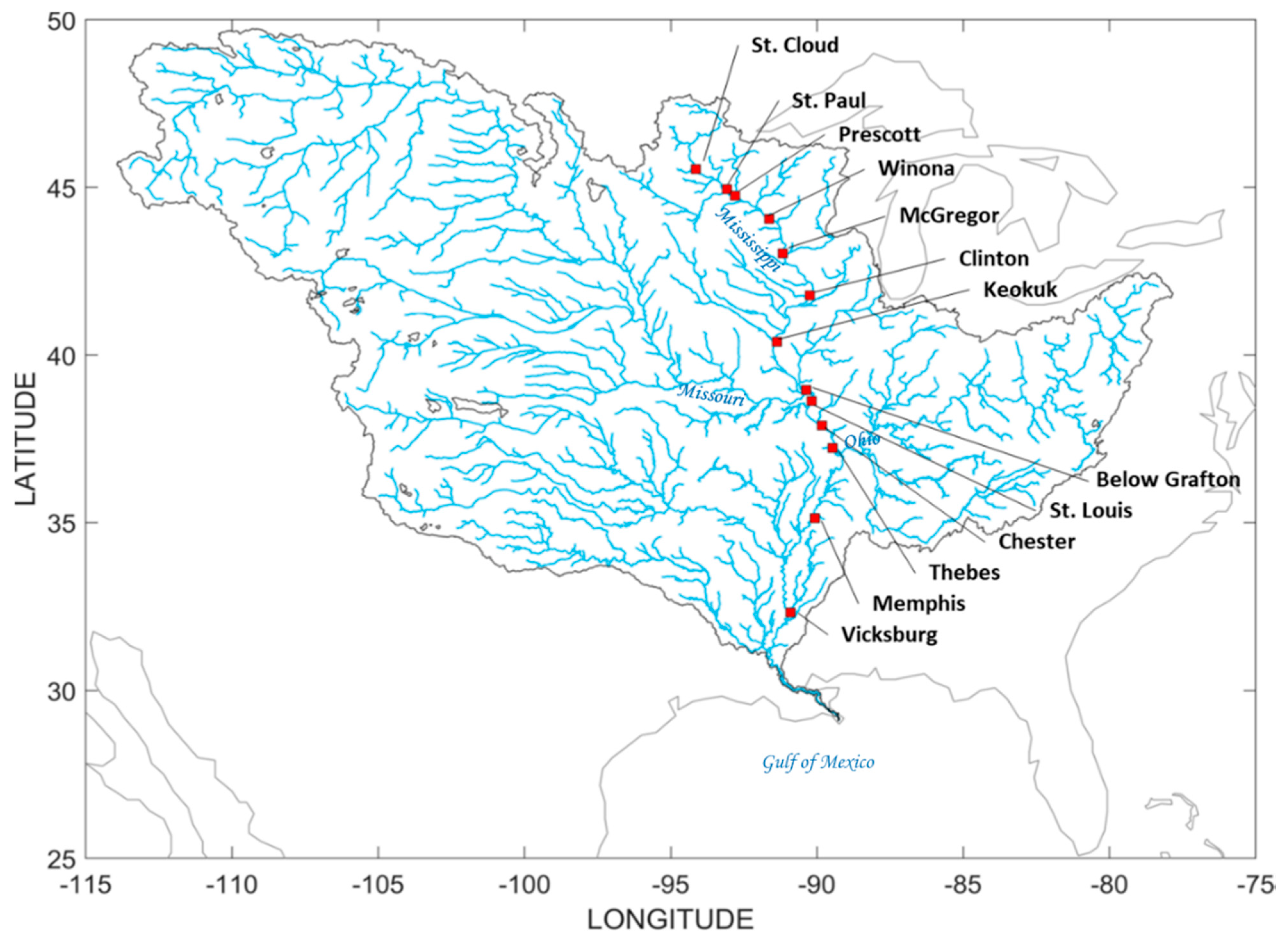
The Mississippi River is the widest basin of the United Stated of America with a surface area of about 3,238,000 km2 and a length of 3770 km, from the headwaters at Lake Itasca, Northern Minnesota, to the mouth in the Gulf of Mexico, Louisiana (6300 km from the source of the Jefferson, at Brower’s Spring) [15]. The Mississippi River can be divided into three parts: The upper Mississippi, which flows from its headwaters at Saint Anthony Falls in Minneapolis to the confluence with the Missouri River, at St. Louis; the middle Mississippi, from St. Luis to the confluence with the Ohio River, at Cairo; and the lower Mississippi, which goes from its confluence with the Ohio River to the river mouth at the Gulf of Mexico. The hydraulic regime is rather complex due to the different tributaries that feed the river and the morphology of the basin: The upper part experiences a pluvial-nival regime, while the lower course crosses a humid subtropical region. Among the main tributaries, the Missouri contributes with a mean flow rate of approximately 2478 m3/s, draining water from the Rocky Mountains, whereas the Ohio River on average supplies the greater flow rate of about 7960 m3/s, draining a vast rainy area from the Appalachian Mountains. Other tributaries are shorter and with variable regimes depending on the heavy rains and cyclones occurring mainly in the coastal zone (see Figure 1).
2.1.1. In Situ Dataset
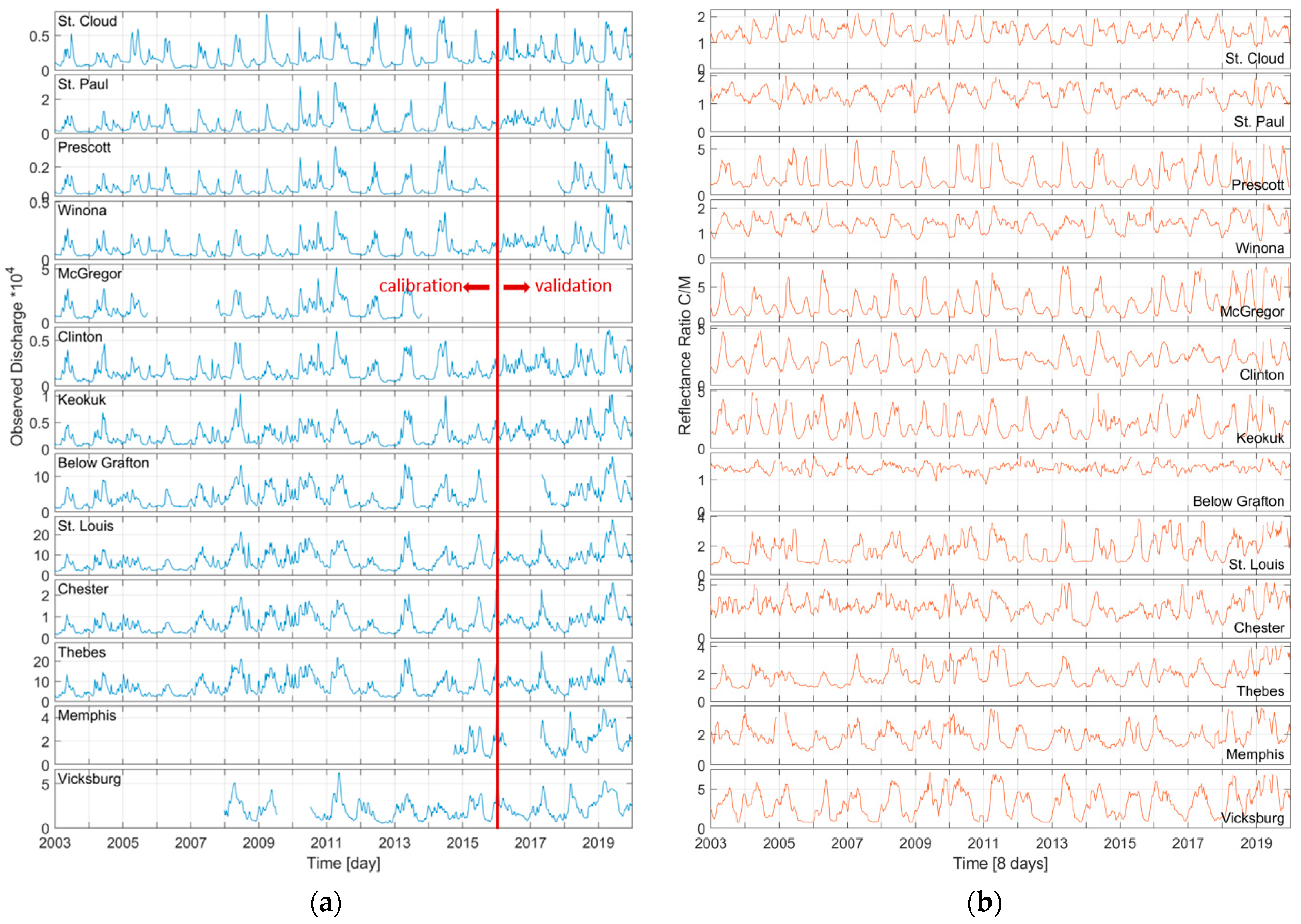
The Mississippi River is monitored along the main course by a series of gauged stations. In this study we consider 13 stations (see Supplementary Material): St. Cloud, St. Paul, Prescott, Winona, Mc Gregor, Clinton, Keokuk, Below Grafton, St. Louis, Chester, Thebes, Memphis, and Vicksburg (see Figure 1). Daily river discharge data are available through the USGS database [16]. In-situ stations have been selected based on the availability of data in the period of interest, which ranges from January 2003 to December 2019, and consistently with the satellite datasets (Table 1). Figure 2a shows the flow hydrographs recorded in the period of analysis at all the considered sites, ordered from upstream to downstream.
2.1.2. Satellite Dataset
MODIS is a multispectral sensor observing the Earth in 36 spectral bands ranging from 405 nm to 14,385 nm. The spatial resolution at the ground depends on the bands: 250 m for band 1 and 2500 m for bands from 3 to 7, and 1 km for the bands from 8 to 36. Here, the MYD09A1 Version 6 product in Near Infrared in band 2 (841–876 nm) is collected, which provides an estimate of the surface spectral reflectance of Aqua MODIS atmospherically corrected every 8 days at 500 m resolution [17]. It is a level-3 composite in which the product pixel contains the best possible Level-2 observation during an 8-day period as selected on the basis of high observation coverage, low view angle, absence of clouds or cloud shadow, and aerosol loading [18]. This product can be considered sufficiently accurate to avoid the presence of the clouds and to investigate most of the selected sites, whose widths exceed 500 m. Only the most upstream stations, St. Cloud and St. Paul, have widths of approximately 180–200 m. For these two stations, the analysis is useful to investigate the limits of applicability of the procedure.
2.2. Methods
The adopted method includes two steps. The first one is the extraction of the reflectance ratio from the MODIS images, and the second one is the building of the FDCs based on satellite and ground data.
2.2.1. Estimation of the Reflectance Ratio
Reflectance is a measure of directly incident light, conventionally expressed as a percentage, which is reflected off a surface. The reflectance depends on the wavelength and assumes different values for different surfaces [19]. In the Near Infrared (NIR), the surface reflectance of wet soil is lower than that of dry soil and for a watercourse it assumes even lower values. For this reason, often NIR is used with Short-wave infrared (SWIR) or visible (through the Normalized Different Water Index, NDWI) to discriminate between water and no water during flood events and inundations [20,21,22,23]. The variation of the moisture content in an area affected by inundations causes a variation of the surface reflectance. Specifically, during a flood event, when the river discharge of a natural channel increases, the water extent increases too, and the riparian zone changes its status from dry to wet. Consequently, the surface reflectance over these areas decreases. If the area is not subject to occasional flood inundation or, more generally, to water content variation, the surface reflectance does not show significant variations. The consideration of the ratio between the dry pixel (C for calibration) and the wet pixel (M for measurement) reduces the effects of vegetation and/or atmosphere existent in both (i.e., wet and dry) pixels signals and provides a clearer signal of water variation, which is expected to be detected with the increasing of river discharge.
The variation of the surface reflectance with the river discharge, or other flow-related variables (i.e., flow velocity, water level, flow area, and water surface) has been already tested in several studies through the analysis with different satellite sensors: Landsat, MODIS, MERIS, OLCI, and Sentinel-2 [11,12,13,14,24,25]. Recently, Tarpanelli et al. [25] demonstrated that the surface reflectance ratio calculated between a dry and a wet pixel is a good estimator of the flow related variables. Here, we propose the same procedure to extract the C/M ratio at each site by carrying out the following steps:
- Cut the MODIS images over a square of size proportional to the width of the river (the side ranges from 0.05 to 0.11 km) and centered on the selected site.
- Calculate the temporal coefficient of variation for every pixel of the box considering the set of available MODIS images.
- Calculate, for each image, the spatial average of the reflectance considering the pixels with the coefficient of variation lower than the 5th percentile; this represents the time series of dry pixel (C) at a given location.
- Select a buffer of 1 km around the river and calculate all possible C/M ratios by considering M values of the pixels within the buffer and the average C obtained at step (3).
- Compare every C/M time series against the discharge recorder by the ground monitoring network and calculate the coefficient of correlation.
- Identify the C/M combination and, hence, M pixel that maximizes the coefficient of correlation.
Finally, once the M and the C pixels are found, the surface reflectance ratio C/M is calculated for all the temporal span of the analysis and filtered with a pass filter (moving window average) in order to obtain the temporal series of satellite data (see Supplementary Material). For a detailed description of the procedure, the reader is invited to read Tarpanelli et al. [25].
Assuming the reflectance ratio as a proxy of the flow variables, and in particular of the river discharge (see e.g., [11,13,25]), in this study, we investigated how and to what extent the C/M ratio can be suitable for the estimation of reliable FDCs and, thus, for the evaluation the hydrological regime of a river.
2.2.2. FDC Estimation
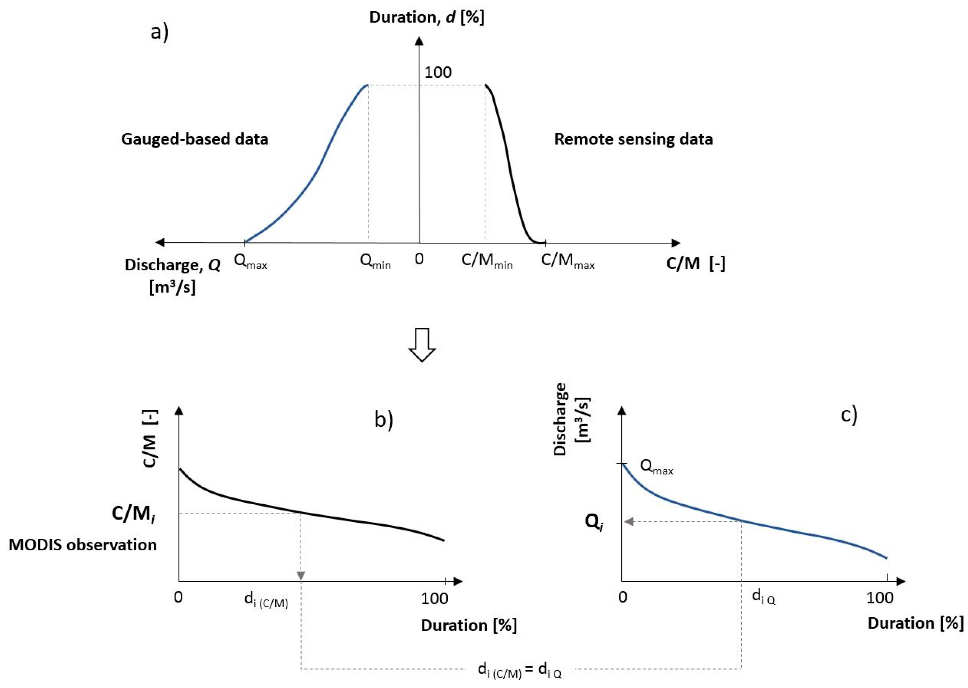
The FDC is an information on the percentage of time that a discharge is equally or exceeded during a reference period, which is, in other terms, an empirical flood frequency distribution of the discharge record. Thus, for each site, the discharge time series are sorted in descending order assigning a corresponding exceeding probability to each value calculated as a percentage of the observation period. Similarly, the same ranking and assignment is done to the C/M series extracted from MODIS images. In this latter case, we refer to the reflectance ratio duration curve, RDC. Because the intent of the current investigation is to evaluate the existence of the potential correlation among RDCs and FDCs, through the probability axes, we assume that, at each site, the discharge and the reflectance ratio are linked to the same exceedance probability. Fitting this link, we can estimate the discharges even if they are no longer available in time, only using the C/M time series. The validity of such assumption is investigated comparing both the discharge temporal series and the FDCs based on observed records and those simulated through C/M values. Figure 3 shows the concept: Panel 3 (a) underlines how RDCs and FDCs are linked by the same frequency axes. This relationship is built in the period of calibration. Panel 3 (b) and 3 (c) show the use of the procedure in the validation period, when the river discharges are not available but can be estimated assuming the same frequency of occurrence of C/M values. Specifically, the analysis is divided in a calibration and validation period. In order to have robust FDCs, a period of 13 years from January 2003 to December 2015 is used for calibration purpose, while the remaining 4 years, from January 2016 to December 2019, are considered for validation.
2.2.3. Data Consistency
The river discharge is available at daily sampling, whereas the selected MODIS product is available every 8 days. This inconsistency on the sampling raises an important issue related to the statistical distribution of the observed discharge that can be different if the complete dataset or only the data averaged in the same period of the MODIS measurements is used. This aspect can potentially affect the performance of the methodology, since the statistical distributions (i.e., frequency distribution) might be different. For this reason, the analysis is carried out also considering the river discharge averaged in the same period of 8 days of the MODIS product. The twofold analysis allows us to understand if the quasi-weekly product could be considered appropriate to estimate the FDC and, hence, the river discharge.
2.3. Evaluation of the Results
The performance of the procedure is quantified through the statistical test of Kolmogorov-Smirnov [26] (k-s), which is a nonparametric hypothesis test that evaluates the difference between the cumulative distribution functions of two sample datasets (i.e., two-sample test; simulated and observed discharge series, in this case). If the two series are from the same continuous distribution, the test fails to reject the null hypothesis at a certain significance level (10% in this study).
Further comparisons are carried out in terms of discharges, and the performances are evaluated by the Pearson correlation coefficient, Rp, and the Spearman (rank) correlation coefficient, Rs. The first evaluates the linear relationship between two datasets, the second their monotonic relationship (whether linear or not). To evaluate the goodness of the simulated time series of river discharge in representing the ground-observed variable, four performance indices are selected:
- Root mean square error, RMSE, the second sample moment of the residuals (or differences) between predicted and observed values. It ranges from 0 (perfect fit) to +∞ (low performances).
- Relative RMSE, rRMSE, defined as:
- Normalized RMSE, NRMSE, defined as:
- The Nash–Sutcliffe efficiency [27], NSE, defined as:
3. Results
This section describes the main results obtained from the analysis. Figure 2 shows river discharge (2 a) and the reflectance ratio C/M (2 b) series extracted at every site. The magnitude of the mean and maximum discharge values does not increase from upstream (upper panel) to downstream (lower panel), because of the number of dikes and dams affecting the flow regime. In general, some flow peaks are maintained along the main course, even if the shape of flow hydrographs changes deeply due to the directly draining basins and the inflows of the tributaries as well. At Memphis, the ground-observed discharge has a long period of missing data during the calibration period. Therefore, the FDC is calibrated considering only the year 2015. At McGregor, the ground discharge series are totally missing in the validation period, therefore the simulated discharges cannot be quantitatively validated. Concerning the reflectance ratios, C/M (Figure 2b), the signal variability is very different from one site to another, showing the highest values at Vicksburg and McGregor and lowest values at St. Cloud, St. Paul, Winona, and Grafton. The shape of the temporal series varies considerable among locations. Perhaps, annual double peak is often present in the upper Mississippi, whereas in the downstream part, a single peak trend is observable in the signal, although this is not in agreement with observed discharge records. These differences can be sources of errors for estimating the discharge and thus FDCs.
3.1. FDCs and RDCs Definition Based on Available Datasets
Since the FDCs are strongly sensitive to extreme events, i.e., periods of very high (floods) or very low (droughts) values of river discharge, they can vary significantly in relation to the periods considered for their construction. To test if such an aspect may affect the results of our investigation, FDCs estimated referring to the period of calibration (13 years; 2003–2015) are compared with those retrieved adopting all available data (17 years; 2003–2019). In addition, a further analysis is carried out to check the consistency of the datasets, based on two sampling options: Daily or eight-day interval, which is compatible with the frequency of the satellite product. The results of both the analyses are illustrated in Figure 4. In the first (4 a) and third column (4 c), Figure 4 shows the FDCs built for (i) the entire observation period (tot), from 2003 to 2019, (ii) for the selected calibration period (cal), from 2003 to 2015 and (iii) for the calibration period, but with an eight-day sampling interval. Because the comparison carried out over the FDCs is not sufficient to gather the discrepancies among the configurations, the second (4 b) and the fourth (4 d) column show the differences in discharge between the FDCs built considering the calibration and the total period, and between the FDCs built in the calibration period, with daily and eight-day sampling.
Although FDCs are quite similar in shape, significant differences emerge in relation to the sampling period (i.e., cal vs. tot), especially for medium to high flows. Here, the k-s test rejects the null hypothesis for all the sites, confirming that the two distributions cannot be considered coming from the same distribution. Generally, looking at the highest discharge values (i.e., low durations), the largest errors are between the 13% and 26%, with the exceptions of McGregor, where the periods are coincident due to the missing data and Chester, for which the errors are higher (up to 32%). At Memphis, the use of one year for the calibration is not sufficient to describe a reliable FDC and the error overcomes the 45%. For low discharge values, the differences between the FDCs are minimal, tending to 0, thus the selection of the period has low impact. Concerning the sampling frequency (every eight days or daily), FDCs are pretty close to each other, with negligible differences (under 11%). The higher error values are obtained at St. Claud and Keokuk stations, with 16% and 14%, respectively. For all sites, the k-s test fails to reject the null hypothesis and therefore the eight-day sampled data can be used instead of the daily series without affecting the distribution of FDCs.
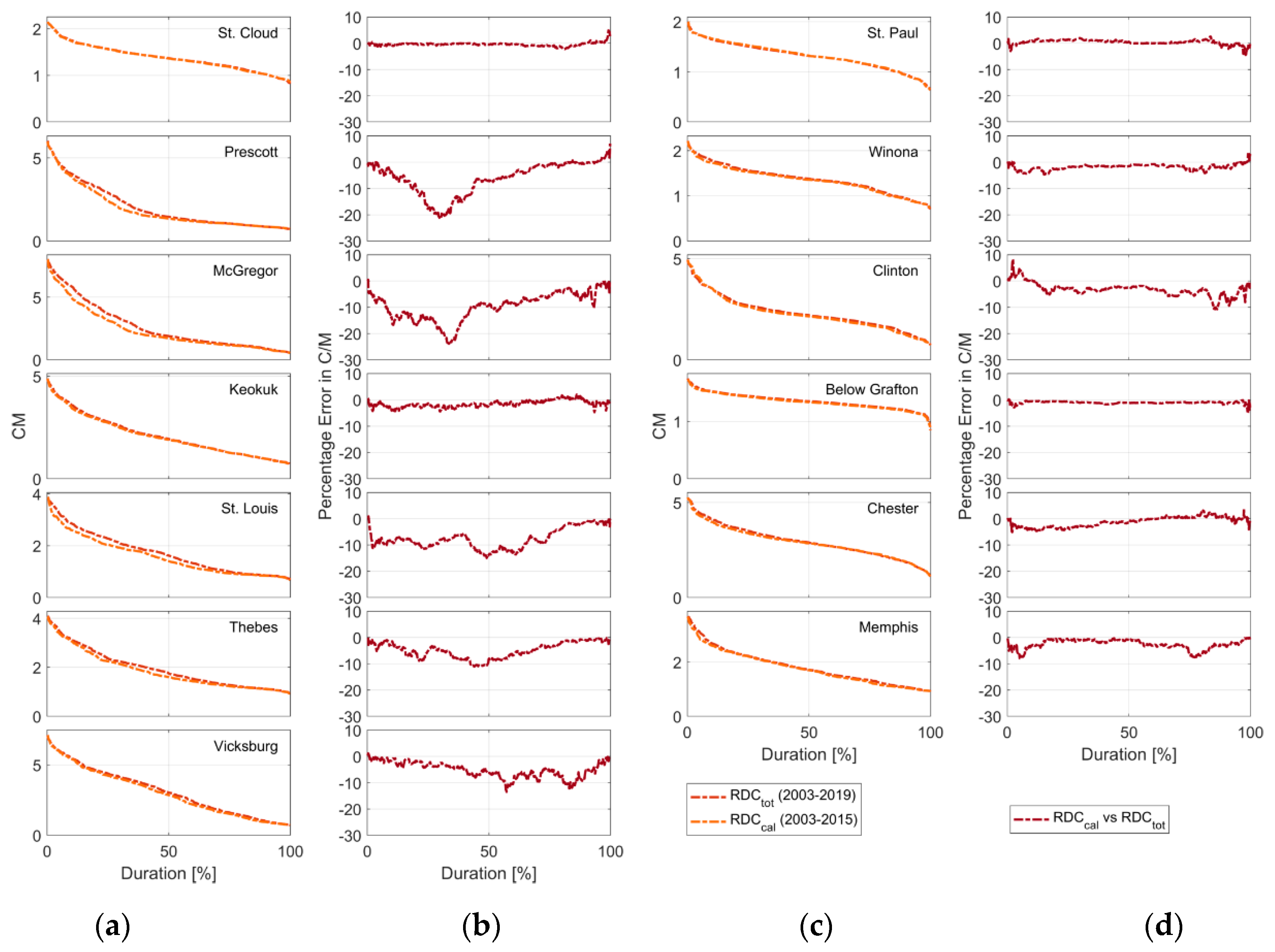
Similarly, Figure 5 represents the RDCs built for the total period (2003–2019) and for the calibration period (2003–2015), at every site. For the reflectance ratio C/M, the differences are more evident in the high values range (duration lower than 50%), tending towards 0 for lower values. As expected, for extreme high events, the RDCs built in the calibration period provide lower values than considering the total period, with the highest errors greater than 20% at Prescott and McGregor, between 10% and 16% at Clinton, St. Louis, Thebes, and Vicksburg, whereas they are less than 10% for the rest of the sites. Despite the differences, the k-s test still fails to reject the null-hypothesis and hence, no big differences are found in the two distributions.
3.2. Comparison in Terms of River Discharge: Calibration Phase
In the phase of calibration, the relationship between FDC and RDC is generated by associating the pairs with the same probability of exceeding and fitting a smoothing spline function. In the validation phase, the reflectance ratio calculated in the corresponding period is then used to derive the discharge values corresponding to the same probability by using the relationships established during the calibration phase (see Figure 3).
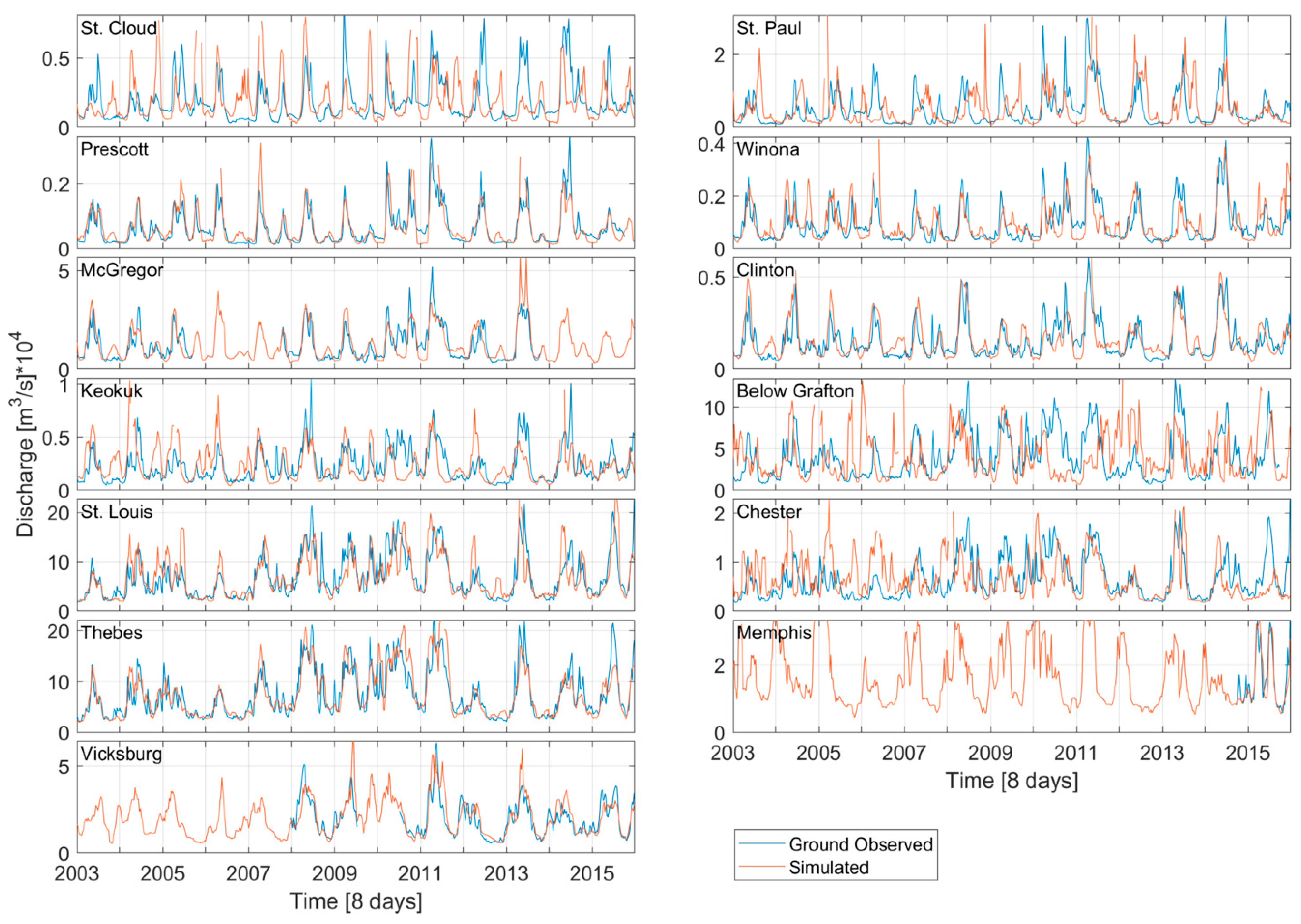
Table 2 reports the performance indices for the calibration phase, while Figure 6 plots the time series. The two upstream sites of St. Cloud and St. Paul do not show good agreement with the observations. At St. Cloud, even if a double peak is detected by the satellite, often the magnitude is completely different, providing errors quite high (around 100% in terms of rRMSE and negative NSE). At St. Paul and Chester, the simulated discharges diverge more in the period 2003–2010, whereas the match is more evident in the period 2011–2015. At Grafton, disagreements are found along the overall period, both in terms of magnitude and in timing of the flood events. At Memphis, the unique year of simultaneous observations provides good performance with high correlations (0.88) and rRMSE rather low (around 25%). At the other stations (Prescott, Winona, McGregor, Clinton, St. Louis, Thebes, and Vicksburg), the simulated and observed river discharges agree: NSE are always positive, NRMSE are in the range of around 10–16%, whereas Spearman correlations are greater than 0.60.
3.3. Comparison in Terms of River Discharge: Validation Phase
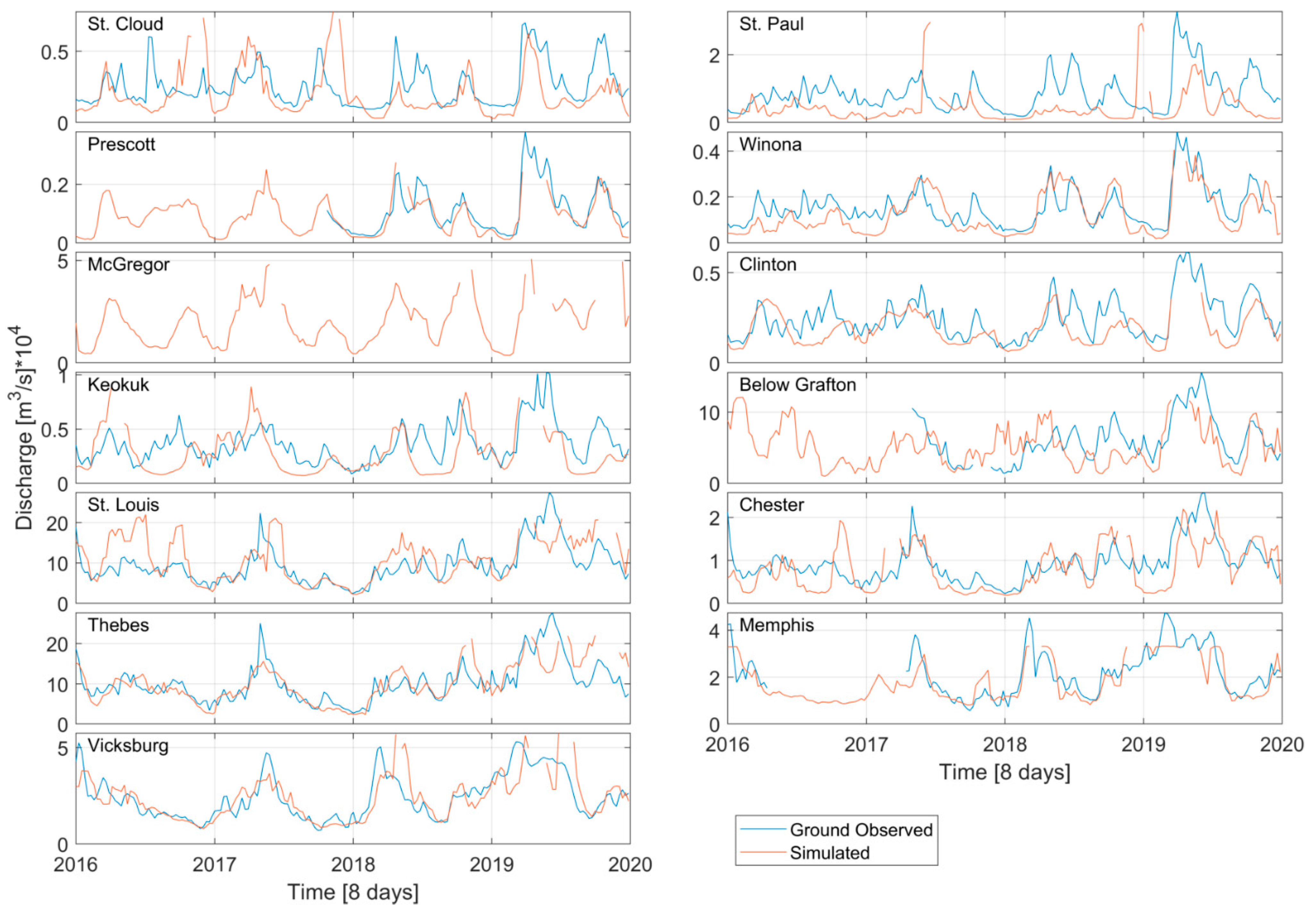
In the validation phase, the same polynomial laws found in the calibration are applied to the reflectance ratio observed in the period 2016–2019. Validation errors are summarized in Table 3, while the discharge time series are shown in Figure 7. The performance indices are globally deteriorated at all sites, with some exceptions. The two upstream stations of St. Cloud and St. Paul also maintain bad performances in the validation period. The same considerations apply for Keokuk, Grafton, and Chester. Unexpectedly, at St. Louis, the simulated discharges that well match the calibration period deviate from the observed discharges in the validation period, especially in 2016 and in 2019, with consequences in the performances: NSE becomes almost null and rRMSE increases up to 52%. For Winona and Clinton, even if in the validation period the performances are worsened, the simulated discharges maintain acceptable results with NSE around 0.29 and rRMSE of about 47 and 41%. Good performances are obtained for Prescott, Thebes, Memphis, and Vicksburg, with NSE in the range 0.42–0.76 and rRMSE between 27% and 40%.
3.4. FDCs in the Validation Phase: Evaluation of the Performances
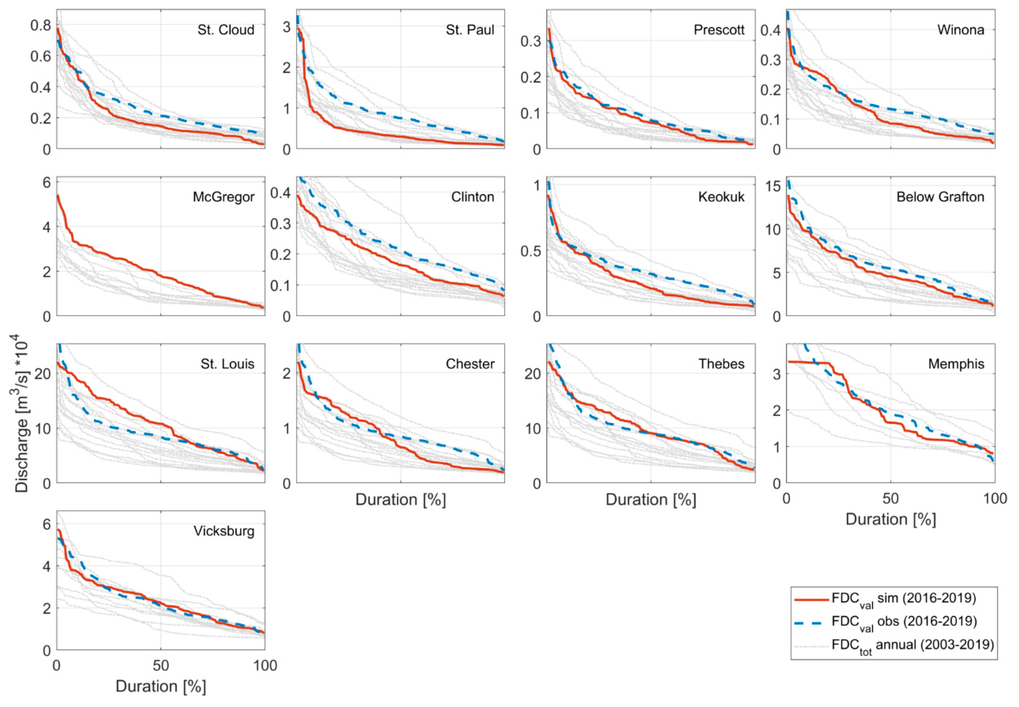
Conscious of such potential performances (expected and in line with previous investigations when trying to reproduce the discharge dynamic in time), the main purpose of the study is not to reproduce the temporal variation of the discharges, rather their frequency distributions over a period of reference. Thus, Figure 8 shows the FDCs built by using the C/M ratio, here called FDCval sim, compared to the FDCs built by the ground-observed data in the same period of validation, FDCval obs. According to the k-s test (significance level alpha equal to 0.01), the flow duration curves simulated for Below Grafton, Thebes, Memphis, and Vicksburg are from the same distribution of those observed. For the other sites, the k-s test failed (k-s rejects the null hypothesis). However, considering the FDCs reconstructed annually for the entire period (2013–2019), we show that the FDCval sim fall within the range of variability of the FDCs (see light gray curves in Figure 8). Thus, although not perfectly in agreement with the observations, FDCval sim can be associated with the natural variability expected for the annual flow duration curves. For McGregor, because in the validation period the data are missing, we compare the simulated FDCs with the annually reconstructed FDCs in the calibration period.
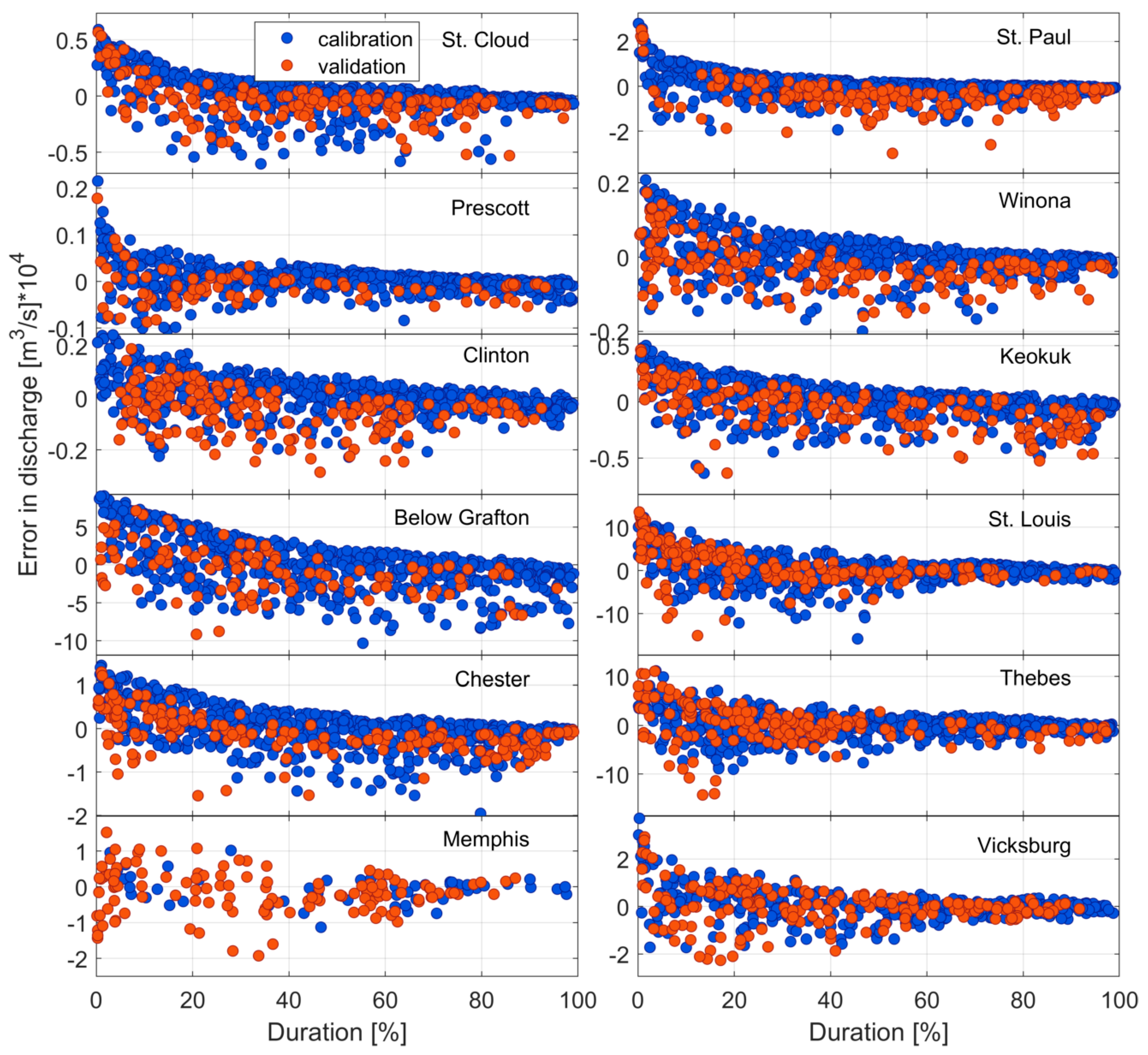
Figure 9 shows the distribution of the errors expressed as differences between the observed and estimated discharges, for all the sites except for McGregor (due to the missing data during the validation period), removing the temporal dimension (i.e., the variability of the discharge in time at a given section). The highest errors are detected for high flows, with a spread distribution of the errors in the low durations range. For medium and high durations (medium and low discharges, respectively), the differences tend towards 0, meaning a higher potential capacity to estimate the discharges associated with medium-low flow conditions.
4. Discussion
By the analysis of the temporal series of the observed discharges, the k-s test and the plots of Figure 4 underlined that the eight-day sampling guaranteed by MODIS can replace the daily time series without a strong effect on the potential evaluation of FDCs, with only exception for very high flows, as depicted at some stations. In fact, during major events, the dynamic of the river is fast enough to attenuate flow peaks, with the possibility of not being caught having an eight-day sampling.
About the choice of the calibration and the validation phases, the distribution of the flood events is quite uniform in time and no substantial differences are found between the calibration (2003–2015) and the total period (2003–2019) of analysis. However, the k-s test does not allow the FDCs built in the calibration period to be assumed valid for all the periods. It is expected that in the validation phase, the error due to new intense flood events is not completely negligible.
The extensive data availability of MODIS appears sufficient to detect the range of variability of the river flows for most of the sites, even though extreme events (e.g., very high or low flows) might never be observed by the satellite due to a number of causes. First, the MYD09A1 product provides an estimate of the surface spectral reflectance selected from all the acquisitions within the eight-day composite on the basis of observation coverage, the absence of clouds or cloud shadow, and solar zenith. This product can be less sensitive to the high/low flows because of the “average” value over the eight-day period. It is expected that a daily and higher resolution product can be beneficial for detecting the low flows even though more investigations are necessary for testing different regime conditions and climatic areas. Second, during drought period, the spatial resolution of the satellite product can limit the capability to detect a sensitive variation of the river flows. The stations selected for the study have widths ranging from 200 m to 1 km, and during the period of low flows, the extension of the water surface into the pixel can provide a limited variation of radiance, hence of reflectance. Third, the cloud coverage during the flood events is an obstacle to the monitoring capacity of the satellite. Consequently, the high flows can be rarely observed and as is known, the underestimation of the flows is expected. However, even if not fully exhaustive during the flood events, the wetted conditions of the areas after a flooded event can last more than one day and, perhaps, it can be detected by other missions orbiting in the same area in a successive period. A multi mission approach can be a solution for a more robust and reliable detection of intense events. A larger availability of multispectral products from several satellite platforms, i.e., Envisat MERIS, Sentinel-3 OLCI, Sentinel-2 MSI, and Landsat family, is expected to increase the frequency of the sampling and, hence, the possibility to monitor even extreme events [25].
Concerning the middle flows, the procedure enables a reliable estimation of the hydraulic regime of the river in the area of interest and may provide useful information for the management of the flows. Indeed, as demonstrated by Figure 6 and Figure 7, the procedure is able to cover periods of ground missing data through the exploitation of satellite information. The overall accuracy on the estimation of the river flows is considered sufficient, even if the evaluation of reliable extreme events is probably the most relevant open issue to deal with. The results of Figure 9 show the good performances for the evaluation of the medium flows and this characteristic encourages the use of the RDC for the management of the water resources. Although errors are still relevant when applying the proposed methodology to reconstruct the discharge series, those biases appear somehow attenuated removing the temporal component, thus focusing more on the frequency of occurrence of the discharge over a period of reference than on its dynamic in time.
This study represents a first attempt to analyze the FDC with a long and easily accessible satellite dataset. However, for the nature of the sensor, it is not possible to totally overtake the intrinsic limit of the passive sensor that is linked to the cloud coverage. In this context, the use of satellite altimetry can be a valuable solution, due to the high level of accuracy it demonstrated in previous works [28,29], especially if multi-mission approaches are used [24,30,31,32]. The merging procedures available in literature [33,34,35] demonstrated the importance and the potential of the combination of more sensors to catch the different aspects of a same phenomenon, which could be helpful for the description of the flow regime.
In particular, the approach proposed here can be profitable under different points of view. The ground observations play an important role in the evaluation of the flow regime of a river. However, due to the not-uniform distribution of the gauged stations in the world, their use should be combined with other source of data with a larger coverage in space and time, like the satellite observations. Because the river discharge is an undirect measurement, so far, no satellite observation is able to derive it directly. However, satellite sensors can provide complementary information. This study showed an example of the use of NIR sensors for providing a reliable frequency of the flow.
For instance, the proposed approach can be used in the case of the decommissioning of a gauging station, ensuring a continuous monitoring of the flows and the estimation of the hydrological regime.
The implementation of this approach at completely ungauged river sites is so far prevented by the calibration phase, which requires concurrent availability of C/M and ground-surveyed discharge series. However, future investigations will be dedicated to trying to overtake such constrains, perhaps considering the possibility to link the existing relationship among Q and C/M to other factors (i.e., topographic, hydrological, etc.) easily available on remote areas. This would definitely improve our capability to estimate the hydrological regime along ungauged rivers.
In addition, the small number of satellite data required by the presented approach (a temporal series of image product) can be considered highly advantageous with respect to hydrological or land surface models that require numerous observations (precipitations, soil moisture, terrestrial water storage) and ancillary data.
5. Conclusions
The scarce availability of long and continuous time series of ground discharges brings the community to enlarge the sources of monitoring englobing the use of satellite remote sensing information. The number of the current satellite missions and their extended spatial and temporal coverage represents a unique opportunity to the global freshwater monitoring of the hydraulic regime, even in poorly gauged areas. The flow duration curves (FDCs) describe the hydraulic regime of the river at specific sites well, providing a cumulative distribution of the flows in terms of percentage of exceedance. Here, we investigated the possibility to describe the hydraulic regime through the reconstruction of FDCs with the use of reflectance ratios from near infrared images, which recently have demonstrated their capability to describe the variability of the river flows with good accuracy [11,12,13,25].
The analysis presented in this work refers to the main course of the Mississippi River, from the upstream section of St. Cloud to the downstream section of Vicksburg, analyzing a total of 13 stations where records of river discharge are available almost for all the analyzed period (2003–2019). We reconstructed the FDCs for the first 13 years and compared them against the reflectance duration curves, RDCs, built from the NIR images of the MODIS product. We validated the FDC for the rest of the four years in terms of temporal river discharges, demonstrating that in most of the cases, the reflectance ratio is able to describe the flow regime at different locations. The good description of the mean river flow for most of the sites highlights the large potential of the NIR sensor to provide precious information at local scale. Higher errors are expected at FDC tails, where very low or high flows cannot be observed by this kind of sensor, due to its passive nature and its medium resolution.
Future applications will investigate the use of multi-mission sensors, perhaps referring to additional NIR sensors and active sensors (i.e., radar altimeters) to ensure a denser temporal frequency and a more reliable and accurate estimation of the extreme (especially high) flows. If we merge the observations retrieved from several NIR sensors (e.g., Landsat, MODIS/Terra and MODIS/Aqua, OLCI/Sentinel-3, and MSI/Sentinel-2 currently available), we have the possibility to densify the time series reaching a frequency almost daily (depending on the clouds). In addition, with the use of radar altimetry, it is possible to overcome the problem of the clouds and obtain a dense time series of water level with the use of multiple tracks and different missions (SARAL/AltiKa, Sentinel-3, Sentinel-6, Jason-3, CryoSat-2, and the future SWOT). The joint use of both the sensors (NIR and radar altimeter) is expected to advance our capability to record high and low discharge peaks, which are fundamental to prevent and forecast extreme events of floods and droughts.
Moreover, the extended applications to other rivers characterized by different hydrological regimes (i.e., big rivers with strong seasonality) could demonstrate a drastic improvement of the results. Indeed, the attempt shown here represents just one example of how the satellite can be used also for ungauged river basin, providing continuous, reliable, and updated information for the management of the flows.
Supplementary Materials
The following are available online at https://0-www-mdpi-com.brum.beds.ac.uk/article/10.3390/app11083458/s1.
Author Contributions
Conceptualization, A.D.; methodology, A.T.; software, A.T.; validation, A.T. and A.D.; formal analysis, A.T.; investigation, A.T. and A.D.; resources, A.T.; data curation, A.T.; writing—original draft preparation, A.T.; writing—review and editing, A.D.; visualization, A.T.; supervision, A.D. All authors have read and agreed to the published version of the manuscript.
Funding
This research received no external funding.
Institutional Review Board Statement
Not applicable.
Informed Consent Statement
Not applicable.
Data Availability Statement
The ground and satellite data and the MATLAB code used for the analysis are available for the reader (see Supplementary Material).
Acknowledgments
The authors wish to thank the USGS for discharge observations and the National Aeronautics and Space Administration, Washington, DC, USA, for providing satellite data.
Conflicts of Interest
The authors declare no conflict of interest.
References
- Vogel, R.M.; Fennessey, N.M. Flow duration curves II: A review of applications in water resources planning 1. JAWRA J. Am. Water Resour. Assoc. 1995, 31, 1029–1039. [Google Scholar] [CrossRef]
- Pugliese, A.; Castellarin, A.; Brath, A. Geostatistical prediction of flow–duration curves in an index-flow framework. Hydrol. Earth Syst. Sci. 2014, 18, 3801–3816. [Google Scholar] [CrossRef] [Green Version]
- Castellarin, A.; Persiano, S.; Pugliese, A.; Aloe, A.; Skøien, J.O.; Pistocchi, A. Prediction of streamflow regimes over large geographical areas: Interpolated flow–duration curves for the Danube region. Hydrol. Sci. J. 2018, 63, 845–861. [Google Scholar] [CrossRef] [Green Version]
- Booker, D.J.; Snelder, T.H. Comparing methods for estimating flow duration curves at ungauged sites. J. Hydrol. 2012, 434–435, 78–94. [Google Scholar] [CrossRef]
- Domeneghetti, A.; Tarpanelli, A.; Grimaldi, L.; Brath, A.; Schumann, G. Flow Duration Curve from Satellite: Potential of a Lifetime SWOT Mission. Remote Sens. 2018, 10, 1107. [Google Scholar] [CrossRef] [Green Version]
- Domeneghetti, A.; Schumann, G.; Tarpanelli, A. Preface: Remote Sensing for Flood Mapping and Monitoring of Flood Dynamics. Remote Sens. 2019, 11, 943. [Google Scholar] [CrossRef] [Green Version]
- Tourian, M.J.; Sneeuw, N.; Bárdossy, A. A quantile function approach to discharge estimation from satellite altimetry (ENVISAT). Water Resour. Res. 2013, 49, 4174–4186. [Google Scholar] [CrossRef]
- Brakenridge, G.R.; Nghiem, S.V.; Anderson, E.; Chien, S. Space-based measurement of river runoff. Eos Trans. AGU 2005, 86, 185–188. [Google Scholar] [CrossRef] [Green Version]
- Tarpanelli, A.; Brocca, L.; Lacava, T.; Melone, F.; Moramarco, T.; Faruolo, M.; Pergola, N.; Tramutoli, V. Toward the estimation of river discharge variations using MODIS data in ungauged basins. Remote Sens. Environ. 2013, 136, 47–55. [Google Scholar] [CrossRef]
- Van Dijk, A.I.J.M.; Brakenridge, G.R.; Kettner, A.J.; Beck, H.E.; De Groeve, T.; Schellekens, J. River gauging at global scale using optical and passive microwave remote sensing. Water Resour. Res. 2016, 52, 6404–6418. [Google Scholar] [CrossRef]
- Li, H.; Li, H.; Wang, J.; Hao, X. Extending the Ability of Near-Infrared Images to Monitor Small River Discharge on the Northeastern Tibetan Plateau. Water Resour. Res. 2019, 55, 8404–8421. [Google Scholar] [CrossRef]
- Shi, Z.; Chen, Y.; Liu, Q.; Huang, C. Discharge Estimation Using Harmonized Landsat and Sentinel-2 Product: Case Studies in the Murray Darling Basin. Remote Sens. 2020, 12, 2810. [Google Scholar] [CrossRef]
- Sahoo, D.P.; Sahoo, B.; Tiwari, M.K. Copula-based probabilistic spectral algorithms for high-frequent streamflow estimation. Remote Sens. Environ. 2020, 251, 112092. [Google Scholar] [CrossRef]
- Tarpanelli, A.; Amarnath, G.; Brocca, L.; Massari, C.; Moramarco, T. Discharge estimation and forecasting by MODIS and altimetry data in Niger-Benue River. Remote Sens. Environ. 2017, 195, 96–106. [Google Scholar] [CrossRef]
- Ghizzoni, T.; Roth, G.; Rudari, R. Multisite flooding hazard assessment in the Upper Mississippi River. J. Hydrol. 2012, 412–413, 101–113. [Google Scholar] [CrossRef]
- United States Geological Survey, USGS. Available online: https://waterdata.usgs.gov/nwis/sw (accessed on 10 January 2021).
- United States Geological Survey, USGS. Available online: https://search.earthdata.nasa.gov/ (accessed on 22 September 2020).
- Vermote, E.F.; Kotchenova, S.Y. MOD09 (Surface Reflectance) User’s Guide, Version 1.1. March 2008. Available online: https://patarnott.com/satsens/pdf/MOD09_UserGuide_v1_2.pdf (accessed on 12 April 2021).
- Huang, C.; Chen, Y.; Zhang, S.; Wu, J. Detecting, extracting, and monitoring surface water from space using optical sensors: A review. Rev. Geophys. 2018, 56, 333–360. [Google Scholar] [CrossRef]
- McFeeters, S.K. The use of the Normalized Difference Water Index (NDWI) in the delineation of open water features. Int. J. Remote Sens. 1996, 17, 1425–1432. [Google Scholar] [CrossRef]
- Yang, X.; Zhao, S.; Qin, X.; Zhao, N.; Liang, L. Mapping of urban surface water bodies from Sentinel-2 MSI imagery at 10 m resolution via NDWI-based image sharpening. Remote Sens. 2017, 9, 596. [Google Scholar] [CrossRef] [Green Version]
- Munasinghe, D.; Cohen, S.; Huang, Y.F.; Tsang, Y.P.; Zhang, J.; Fang, Z. Intercomparison of Satellite Remote Sensing-Based Flood Inundation Mapping Techniques. JAWRA J. Am. Water Resour. Assoc. 2018, 54, 834–846. [Google Scholar] [CrossRef]
- Nandi, I.; Srivastava, P.K.; Shah, K. Floodplain mapping through support vector machine and optical/infrared images from Landsat 8 OLI/TIRS sensors: Case study from Varanasi. Water Resour. Manag. 2017, 31, 1157–1171. [Google Scholar] [CrossRef]
- Tarpanelli, A.; Santi, E.; Tourian, M.J.; Filippucci, P.; Amarnath, G.; Brocca, L. Daily river discharge estimates by merging satellite optical sensors and radar altimetry through artificial neural network. IEEE Trans. Geosci. Remote 2018, 57, 329–341. [Google Scholar] [CrossRef]
- Tarpanelli, A.; Iodice, F.; Brocca, L.; Restano, M.; Benveniste, J. River flow monitoring by Sentinel-3 OLCI and MODIS: Comparison and combination. Remote Sens. 2020, 12, 3867. [Google Scholar] [CrossRef]
- Massey, F.J. The Kolmogorov-Smirnov Test for Goodness of Fit. J. Am. Stat. Assoc. 1951, 46, 68–78. [Google Scholar] [CrossRef]
- Nash, J.E.; Sutcliffe, J.V. River flow forecasting through conceptual models, part I: A discussion of principles. J. Hydrol. 1970, 10, 282–290. [Google Scholar] [CrossRef]
- Paris, A.; Dias de Paiva, R.; Santos da Silva, J.; Medeiros Moreira, D.; Calmant, S.; Garambois, P.-A.; Collischonn, W.; Bonnet, M.-P.; Seyler, F. Stage-discharge rating curves based on satellite altimetry and modeled discharge in the Amazon basin. Water Resour. Res. 2016, 52, 3787–3814. [Google Scholar] [CrossRef] [Green Version]
- Zakharova, E.A.; Krylenko, I.N.; Kouraev, A.V. Use of non-polar orbiting satellite radar altimeters of the Jason series for estimation of river input to the Arctic Ocean. J. Hydrol. 2019, 568, 322–333. [Google Scholar] [CrossRef]
- Tourian, M.J.; Tarpanelli, A.; Elmi, O.; Qin, T.; Brocca, L.; Moramarco, T.; Sneeuw, N. Spatiotemporal densification of river water level time series by multimission satellite altimetry. Water Resour. Res. 2016, 52. [Google Scholar] [CrossRef] [Green Version]
- Tourian, M.J.; Schwatke, C.; Sneeuw, N. River discharge estimation at daily resolution from satellite altimetry over an entire river basin. J. Hydrol. 2017, 546, 230–247. [Google Scholar] [CrossRef]
- Boergens, E.; Dettmering, D.; Seitz, F. Observing water level extremes in the Mekong River Basin: The benefit of long-repeat orbit missions in a multi-mission satellite altimetry approach. J. Hydrol. 2019, 570463–570472. [Google Scholar] [CrossRef] [Green Version]
- Tarpanelli, A.; Brocca, L.; Barbetta, S.; Faruolo, M.; Lacava, T.; Moramarco, T. Coupling MODIS and Radar Altimetry Data for Discharge Estimation in Poorly Gauged River Basins. IEEE J. Sel. Top. Appl. 2015, 8, 141–148. [Google Scholar] [CrossRef]
- Sichangi, A.W.; Wang, L.; Yang, K.; Chen, D.; Wang, Z.; Li, X.; Zhou, J.; Liu, W.; Kuria, D. Estimating continental river basin discharges using multiple remote sensing data sets. Remote Sens. Environ. 2016, 179, 36–53. [Google Scholar] [CrossRef] [Green Version]
- Huang, Q.; Lond, D.; Mingda, D.; Zeng, C.; Qiao, G.; Li, X.; Hou, A.; Hong, Y. Discharge estimation in high-mountain regions with improved methods using multisource remote sensing: A case study of the Upper Brahmaputra river. Remote Sens. Environ. 2018, 219, 115–134. [Google Scholar] [CrossRef]
Figure 1.
Geographical location of the Mississippi River, including spatial distribution of in-situ stations used in this study.
Figure 1.
Geographical location of the Mississippi River, including spatial distribution of in-situ stations used in this study.

Figure 2.
River discharge hydrograph (a) and reflectance ratio C/M (b) for the selected in-situ gauged stations.
Figure 2.
River discharge hydrograph (a) and reflectance ratio C/M (b) for the selected in-situ gauged stations.

Figure 3.
Conceptual scheme of the procedure between ground-based and remote sensing data. (a) schematic representation of the relationship between Discharge Q and remote sensing data, C/M through their duration; duration curve in terms of remote sensing, C/M (b) and discharge Q (c).
Figure 3.
Conceptual scheme of the procedure between ground-based and remote sensing data. (a) schematic representation of the relationship between Discharge Q and remote sensing data, C/M through their duration; duration curve in terms of remote sensing, C/M (b) and discharge Q (c).

Figure 4.
(a,c) show flow duration curves (FDCs) calculated for (i) the entire period (tot), from 2003 to 2019, (ii) for the selected calibration period (cal), from 2003 to 2015, and (iii) for the calibration period adopting an eight-day sampling interval for all the sites analyzed. (b,d) columns show differences in discharge between the FDCs built referring to the calibration and total period, and between the FDCs built in the calibration period, but in case of considering daily or eight-day sampling intervals.

Figure 5.
(a,c) show reflectance ratio duration curves (RDCs) calculated for (i) the entire period (tot), from 2003 to 2019, and (ii) for the selected calibration period (cal), from 2003 to 2015. (b,d) columns show differences in reflectance ratio C/M between the RDCs built considering the calibration and the total period, for all the sites analyzed.

Figure 6.
Calibration phase: Comparison between the observed and simulated discharges.

Figure 7.
Validation phase: Comparison between the observed and simulated discharges.

Figure 8.
Simulated and observed FDCs for the period of validation (2016–2019). For comparison, the FDC built on single years of the entire observation period, 2003–2019, are also represented.
Figure 8.
Simulated and observed FDCs for the period of validation (2016–2019). For comparison, the FDC built on single years of the entire observation period, 2003–2019, are also represented.

Figure 9.
Errors between estimated and observed discharges in function of the duration.


Table 1.
List of the in-situ gauged stations along the Mississippi River selected for the analysis (latitude, Lat.; longitude, Lon.; basin area, Ab) and their characteristics (percent of missing data; minimum, maximum and mean river discharge: Qmin, Qmax, and Qmean, respectively) extracted for the period January 2003 to December 2019.
| Station | USGS ID | Lat. | Lon. | Ab [km2] | Missing Data [%] | Qmax [m3/s] | Qmin [m3/s] | Qmean [m3/s] |
|---|---|---|---|---|---|---|---|---|
| St. Cloud | 5270700 | 45.547 | −94.147 | 34,498 | 0 | 10,333 | 277 | 2040 |
| St. Paul | 5331000 | 44.945 | −93.084 | 95,311 | 0 | 35,052 | 622 | 5847 |
| Prescott | 5344500 | 44.746 | −92.800 | 116,031 | 12.0 | 4049 | 108 | 705 |
| Winona | 5378500 | 44.056 | −91.638 | 153,327 | 0.3 | 5040 | 173 | 1076 |
| McGregor | 5389500 | 43.027 | −91.171 | 174,823 | 48.1 | 55,169 | 2213 | 12,333 |
| Clinton | 5420500 | 41.781 | −90.252 | 221,702 | 0 | 6654 | 238 | 1771 |
| Keokuk | 5474500 | 40.394 | −91.374 | 308,207 | 0 | 15,121 | 229 | 2635 |
| Below Grafton | 5587455 | 38.951 | −90.373 | 443,663 | 10.2 | 159,106 | 4084 | 43,651 |
| St. Louis | 7010000 | 38.628 | −90.181 | 1,805,213 | 0 | 283,769 | 16,459 | 74,299 |
| Chester | 7020500 | 37.901 | −89.830 | 1,835,256 | 0 | 27,014 | 1620 | 7202 |
| Thebes | 7022000 | 37.220 | −89.467 | 1,847,170 | 0 | 295,961 | 19,050 | 80,995 |
| Memphis | 7032000 | 35.127 | −90.079 | 2,415,929 | 75.0 | 48,988 | 5097 | 20,250 |
| Vicksburg | 7289000 | 32.315 | −90.906 | 2,964,227 | 35.3 | 65,412 | 5409 | 21,415 |
Table 2.
Calibration phase: Performance indices of the comparison between the observed and simulated discharges: Pearson correlation coefficient, Rp, Spearman correlation coefficient, Rs, Root Mean Square Error, RMSE, Relative RMSE, rRMSE and Nash–Sutcliffe efficiency, NSE.
Table 2.
Calibration phase: Performance indices of the comparison between the observed and simulated discharges: Pearson correlation coefficient, Rp, Spearman correlation coefficient, Rs, Root Mean Square Error, RMSE, Relative RMSE, rRMSE and Nash–Sutcliffe efficiency, NSE.
| Station | Rp [-] | Rs [-] | RMSE [m3/s] | rRMSE [%] | NRMSE [%] | NSE [-] |
|---|---|---|---|---|---|---|
| St. Cloud | 0.29 | 0.37 | 1789 | 95.8 | 23.3 | −0.38 |
| St. Paul | 0.37 | 0.36 | 5502 | 111.2 | 18.6 | −0.24 |
| Prescott | 0.82 | 0.76 | 316 | 50.3 | 9.5 | 0.67 |
| Winona | 0.66 | 0.62 | 571 | 61.3 | 14.1 | 0.36 |
| McGregor | 0.78 | 0.71 | 5763 | 46.9 | 11.8 | 0.53 |
| Clinton | 0.75 | 0.66 | 700 | 45.1 | 12.4 | 0.53 |
| Keokuk | 0.46 | 0.49 | 1654 | 70.9 | 16.4 | −0.06 |
| Below Grafton | 0.16 | 0.17 | 35,301 | 88.0 | 27.8 | −0.64 |
| St. Louis | 0.73 | 0.83 | 31,574 | 46.5 | 15.4 | 0.46 |
| Chester | 0.30 | 0.40 | 4880 | 74.2 | 23.4 | −0.38 |
| Thebes | 0.85 | 0.88 | 25,535 | 34.4 | 12.7 | 0.69 |
| Memphis | 0.90 | 0.90 | 3854 | 24.4 | 14.0 | 0.77 |
| Vicksburg | 0.80 | 0.88 | 7059 | 35.7 | 12.3 | 0.55 |
Table 3.
Validation phase: Performance indices of the comparison between the observed and simulated discharges: Pearson correlation coefficient, Rp, Spearman correlation coefficient, Rs, Root Mean Square Error, RMSE, Relative RMSE, rRMSE and Nash–Sutcliffe efficiency, NSE.
Table 3.
Validation phase: Performance indices of the comparison between the observed and simulated discharges: Pearson correlation coefficient, Rp, Spearman correlation coefficient, Rs, Root Mean Square Error, RMSE, Relative RMSE, rRMSE and Nash–Sutcliffe efficiency, NSE.
| Station | Rp [-] | Rs [-] | RMSE [m3/s] | rRMSE [%] | NRMSE [%] | NSE [-] |
|---|---|---|---|---|---|---|
| St. Cloud | 0.39 | 0.55 | 17,843 | 69.2 | 29.5 | −0.53 |
| St. Paul | 0.14 | 0.31 | 83,784 | 96.5 | 27.2 | −1.20 |
| Prescott | 0.85 | 0.90 | 3815 | 33.7 | 10.7 | 0.79 |
| Winona | 0.73 | 0.74 | 6725 | 43.7 | 15.5 | 0.36 |
| McGregor | - | - | - | - | - | - |
| Clinton | 0.57 | 0.58 | 9768 | 39.7 | 18.3 | 0.32 |
| Keokuk | 0.40 | 0.35 | 20,709 | 57.6 | 22.1 | −0.31 |
| Below Grafton | 0.44 | 0.33 | 326,920 | 54.2 | 23.1 | −0.03 |
| St. Louis | 0.57 | 0.74 | 489,400 | 51.7 | 19.6 | −0.03 |
| Chester | 0.58 | 0.65 | 47,113 | 51.2 | 20.0 | −0.04 |
| Thebes | 0.69 | 0.79 | 382,943 | 37.4 | 15.3 | 0.44 |
| Memphis | 0.81 | 0.84 | 61,406 | 27.8 | 14.7 | 0.66 |
| Vicksburg | 0.72 | 0.82 | 82,228 | 33.8 | 17.9 | 0.52 |
Publisher’s Note: MDPI stays neutral with regard to jurisdictional claims in published maps and institutional affiliations. |
© 2021 by the authors. Licensee MDPI, Basel, Switzerland. This article is an open access article distributed under the terms and conditions of the Creative Commons Attribution (CC BY) license (https://creativecommons.org/licenses/by/4.0/).
Share and Cite
MDPI and ACS Style
Tarpanelli, A.; Domeneghetti, A. Flow Duration Curves from Surface Reflectance in the Near Infrared Band. Appl. Sci. 2021, 11, 3458. https://0-doi-org.brum.beds.ac.uk/10.3390/app11083458
AMA Style
Tarpanelli A, Domeneghetti A. Flow Duration Curves from Surface Reflectance in the Near Infrared Band. Applied Sciences. 2021; 11(8):3458. https://0-doi-org.brum.beds.ac.uk/10.3390/app11083458
Chicago/Turabian StyleTarpanelli, Angelica, and Alessio Domeneghetti. 2021. "Flow Duration Curves from Surface Reflectance in the Near Infrared Band" Applied Sciences 11, no. 8: 3458. https://0-doi-org.brum.beds.ac.uk/10.3390/app11083458
Note that from the first issue of 2016, this journal uses article numbers instead of page numbers. See further details here.