
Straight Gait Research of a Small Electric Hexapod Robot


State Key Laboratory of Fluid Power and Mechatronic Systems, Zhejiang University, Hangzhou 310027, China
*
Author to whom correspondence should be addressed.
Appl. Sci. 2021, 11(8), 3714; https://0-doi-org.brum.beds.ac.uk/10.3390/app11083714
Submission received: 24 March 2021
/
Revised: 15 April 2021
/
Accepted: 17 April 2021
/
Published: 20 April 2021
(This article belongs to the Section Robotics and Automation)
Abstract
:Gait is an important research content of hexapod robots. To better improve the motion performance of hexapod robots, many researchers have adopted some high-cost sensors or complex gait control algorithms. This paper studies the straight gait of a small electric hexapod robot with a low cost, which can be used in daily life. The strategy of “increasing duty factor” is put forward in the gait planning, which aims to reduce foot sliding and attitude fluctuation in robot motion. The straight gaits of the robot include tripod gait, quadrangular gait, and pentagonal gait, which can be described conveniently by discretization and a time sequence diagram. In order to facilitate the user to control the robot to achieve all kinds of motion, an online gait transformation algorithm based on the adjustment of foot positions is proposed. In addition, according to the feedback of the actual attitude information, a yaw angle correction algorithm based on kinematics analysis and PD controller is designed to reduce the motion error of the robot. The experiments show that the designed gait planning scheme and control algorithm are effective, and the robot can achieve the expected motion. The RMSE of the row, pitch, and yaw angle was reduced by 35%, 25%, and 12%, respectively, using the “increasing duty factor” strategy, and the yaw angle was limited in the range −3°~3° using the yaw angle correction algorithm. Finally, the comparison with related works and the limitations are discussed.
1. Introduction
With the advent of the artificial intelligence era, robots are more closely related to human society [1]. Compared with wheeled robots, legged robots have better terrain adaptivity and flexibility, which can complete specific tasks [2]. A hexapod robot is a typical legged robot. When the hexapod robot moves, it has at least three support legs, which is conducive to obtain stability and fault tolerance movement [3]. Meanwhile, compared with bipedal and quadruped robots, hexapod robots are generally easier to control to obtain static stable walking [4]. Looking back, there were great achievements in the field of hexapod robots. Genghis [5] was designed by MIT to detect outer space ground in 1989. Each leg of this small hexapod robot has a rotation joint with 2DOF. Since then, many typical hexapod robots have been designed, such as CWRU [6], DLR Crawler [7], HITCR–II [8], LCR200 [9], etc. The above robots are all driven by electric motors. This mode generally has high efficiency and good controllability [10]. Of course, some typical hexapod robots are driven in other ways. Chiba University’s COMET-IV [11] and NTUA’s HexaTerra [12] are typical hydraulically driven hexapod robots. With their huge size and strong load capacity, they can be used in situations with complex terrain to perform specific tasks. Overall, the structure and control systems of hexapod robots are even more mature. Meanwhile, research of hexapod robots pays more attention to the perception of the environment as well as the improvement of the human–machine interaction experience [13].
A hexapod robot is a complex machine consisting of many actuators, sensors, microcontrollers, and other devices [14]. At present, most hexapod robots are still used on specific occasions. Their complex control systems and algorithms may cause high research costs. This paper designs a small electric hexapod robot for daily life called HexWalker II, which can be used in the fields of education, entertainment, investigation, and so on. We strive to make the robot have good performance and is easy to control under the condition of ensuring low development costs, to shorten the distance between the hexapod robot and people’s lives, which is meaningful in the present era.
Many factors need to be considered when designing a hexapod robot, including mechanism, control architecture, and control algorithm [15], among which gait planning is the key [4]. A gait can be described as a sequence of leg motions coordinated with a sequence of body motions for transporting the robot’s body to move [16]. The study of robot gait is important for improving the stability and flexibility of motion, adapting to different terrains, optimizing energy consumption, and so on. This paper focuses on the research of straight gait planning of the hexapod robot. The robot in this paper adopts periodic gaits, including tripod gait, quadrangular gait, and pentagonal gait. By making improvements on the basis of the traditional hexapod robot gait planning method, a comprehensive gait planning scheme was designed. To further improve the reliability of robot motion, a simple and effective yaw angle correction algorithm is proposed based on kinematics analysis and the PD controller. Finally, the experimental results verify the rationality of the gait planning scheme and motion control algorithm. This paper makes the following contributions:
- Compared to the traditional hexapod robot gait planning method, the strategy “increasing duty factor” is introduced to ensure the stability of robot motion;
- All kinds of gaits are described based on the discretization and time sequence diagram, and the robot gait conversion scheme is designed. This is so that the robot can flexibly transform among various gaits to ensure the integrity and coordination of the motion, which is less studied in the previous research;
- A yaw angle correction algorithm is proposed based on kinematics analysis and the PD controller to reduce the motion error of the robot.
2. Related Work
The gaits of hexapod robots include periodic gait and free gait. The periodic gait is easy to control, which enables the robot to achieve various movements accurately according to the actual situation or the needs of the user. Therefore, it is especially widely used in relatively flat and simple environments [17]. The free gait is different from the periodic gait, that is, the legs of the multi-legged robot no longer have a strict periodic swing sequence. The generation of free gait is usually generated according to a series of rules, such as Cruse’s rules [18], which are adopted by DLR Crawler [19]. The gaits of the hexapod robot in Reference [20] are generated by the CPG network. The robot can adjust the parameters of the network through the PD controller according to the feedback of the attitude angle to realize the attitude compensation in the motion, which is verified by simulation. Free gait may be convenient for the robot to adjust the motion state of each leg timely to adapt to complex terrain, but its calculation is more complicated and its controllability is relatively poor.
When the hexapod robot walks straight, the attitude may fluctuate due to mechanical error, foot slipping, and other factors. Therefore, it is necessary to adopt some more control strategies to improve the motion performance of the robot. The six-legged walking robot platform designed by ZJU has three joints and a semi-round foot on each leg. Based on the inverse velocity kinematics, the research team has studied the posture control strategy to improve the walking ability of the robot on rough terrain [21]. Based on the study of mechanics, Reference [22] realizes the closed-loop control of the posture by distributing the foot force to reduce energy consumption and ensure the stability of the hexapod robot. However, these algorithms may require high performance of control system hardware, which may be difficult to implement.
Recent researches on hexapod robot gait include optimization of gait energy consumption, gait planning over uneven terrain, and so on. Reference [23] analyzed the energy consumption of different gaits. It proposed a heuristic algorithm to switch gait based on the current speed, which can take full advantage of the gait diversity for a hexapod robot. Based on tactile sensors, References [24,25] designed leg trajectories for traversing obstacles and optimized the energy efficiency for trajectory transformation. Reference [26] optimized the mechanical structure and gait parameters simultaneously for a hydraulic hexapod robot to minimize energy consumption. Although energy optimization and obstacle traversing are not studied in this paper, these are good applications and research directions for gait conversion of a hexapod robot.
3. Basic Control Method of the Robot
3.1. Control System
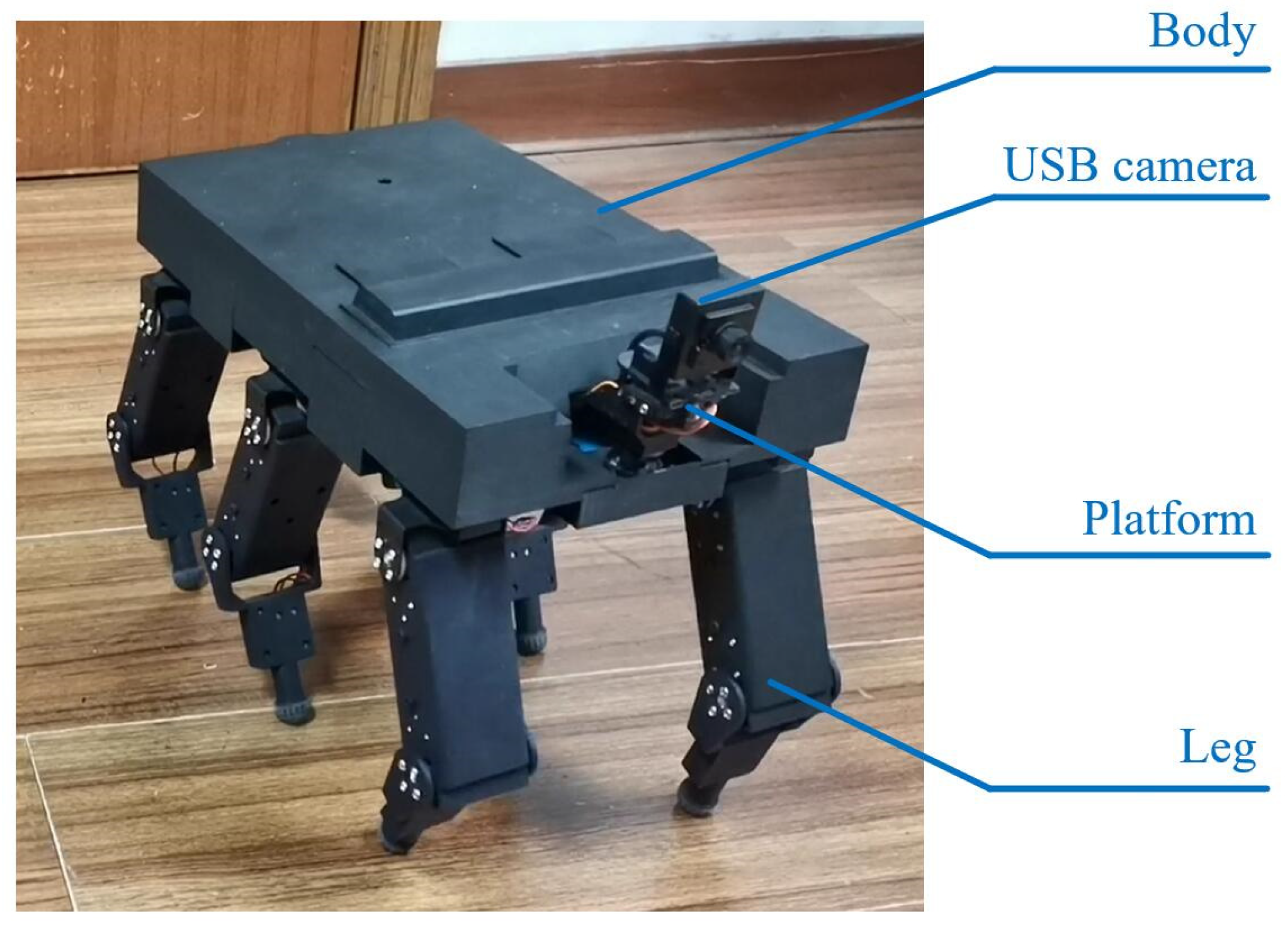
The picture of HexWalker II is shown in Figure 1. The dimensions of the robot are 268 mm × 166 mm × 275 mm, and the weight of the robot is around 3 kg. The axis of the root joint is parallel to the body of the robot. The legs are entirely under the body, not the side. The design imitates mammalian structure, which is more conducive to the realization of the small ground occupation and strong load-bearing capacity [27]. The robot has a 2DOF platform with a USB camera, which can monitor a wide range of video images. Each joint of the robot is actuated by a servo. The servo is a Digital Robot Servo with a 6 V power supply and 15 kg·cm torque output. The rotation angle of each servo can be controlled by sending commands through the serial port based on the set communication protocol. Meanwhile, the servo also supports the function of angle back reading, which means it can provide feedback on its current angle.
The system of the robot includes two parts: the robot part and the remote control part. The remote control part is a mobile device implemented with human–machine interface software, which can help the user send commands to control the robot’s motion and watch the video collected by the USB camera on the robot. The controller on the robot contains two layers to improve the real-time performance of the system. The upper layer is Raspberry Pi 3B+, which runs the core control algorithm of the robot and communicates with the remote control part through the network. The lower layer is a self-designed embedded system, which mainly realizes the functions of joint actuating and signal acquisition. It communicates with the IMU module through the serial port to obtain the actual attitude information of the robot.
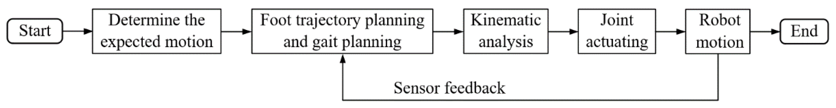
Figure 2 shows the main research contents of the robot’s core control algorithm. According to the requirements, the foot trajectory planning and gait planning scheme is designed to determine the desired position of each foot at each time. Foot trajectory planning and gait planning are based on body modeling and can be adjusted with sensor feedback. Combined with the results of kinematics analysis, the angle commands of each joint needed by the robot to achieve the specified motion can be obtained, which can be used to drive the servo to control the motion of the hexapod robot.
3.2. Kinematic Analysis
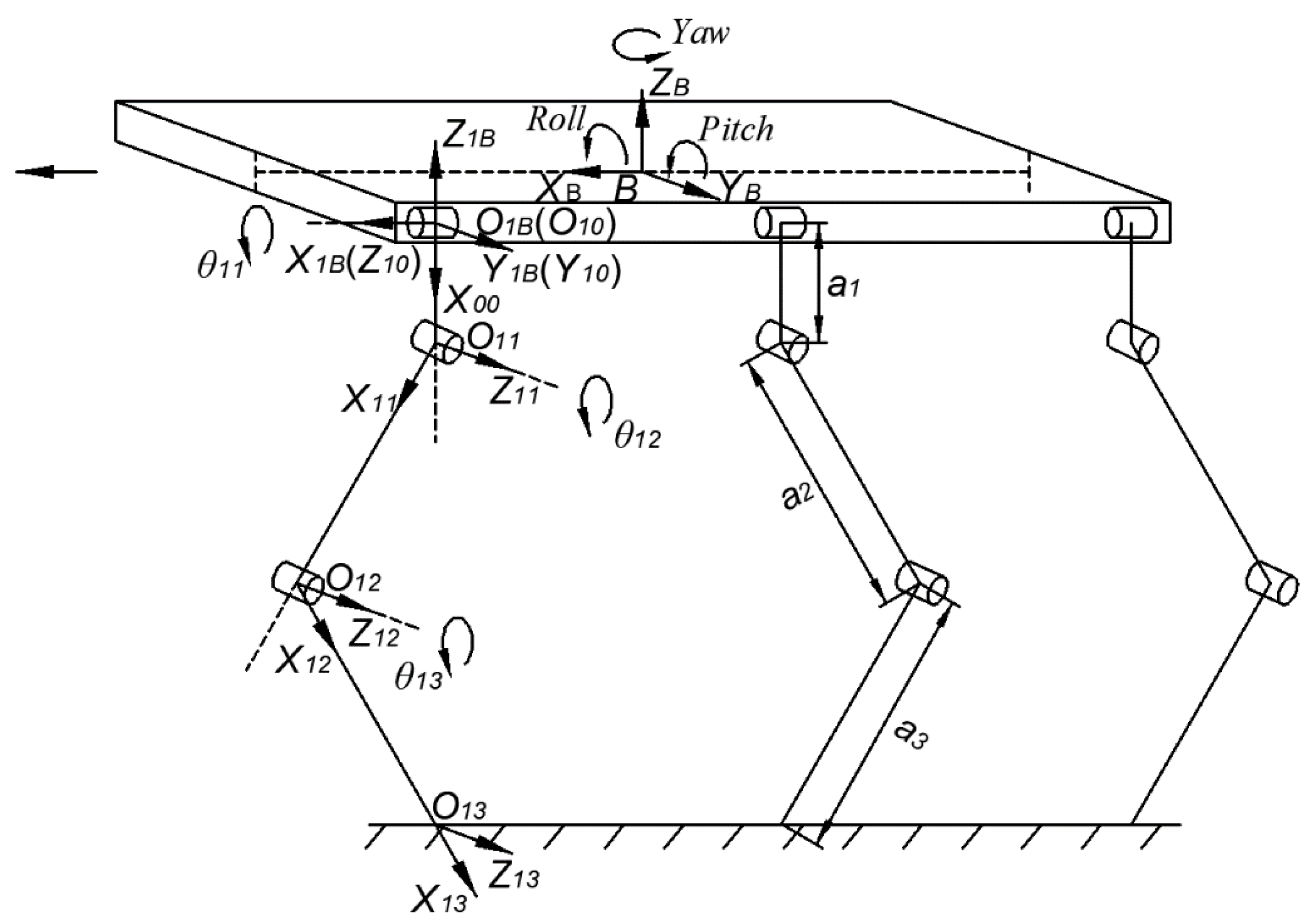
As Figure 3 shows, the body coordinate frame is noted as {B}, which is located at the center of the body and is fixedly connected with the robot. XB points to the forward direction, while ZB is perpendicular to the upper surface of the robot body and points upwards. The direction of YB can be determined by the right-hand rule. The sequence numbers of the robot’s legs are represented by i (i = 1~6). There is a coordinate frame named {OiB} fixed on the center of each leg’s root joint. The directions of coordinate axes are consistent with {B}. {Oi0}, {Oi1}, {Oi2}, {Oi3} represent the coordinate frame of each link of the leg, which are established according to D–H rules [28]. Figure 3 takes leg 1 as an example. The D–H parameters of leg 1 are listed in Table 1. According to the actual situation of the robot, the length of three links (, , ) and the angle range of three joints (, , ) are shown in Table 2.
Based on the D–H parameters, the homogeneous transformation between coordinate systems of adjacent links can be calculated, and the following results can be finally obtained.
where P1x, P1y, and P1z represent the foot position of leg 1 relative to the coordinate system {O1B}. Of course, the foot position in the body coordinate frame {B} can be obtained easily. This is the process of forward kinematic analysis.
According to the position of the foot, inverse kinematic analysis can calculate the angle of each joint of the leg, which is the basis of controlling the robot’s motion. Based on the forward kinematic analysis and mathematical derivation, the inverse kinematic equations can be given as follows:
Due to the different leg bending directions, is positive for the front legs (i = 1, 2), but negative for the middle and rear legs (i = 3, 4, 5, 6).
3.3. Foot Trajectory Planning
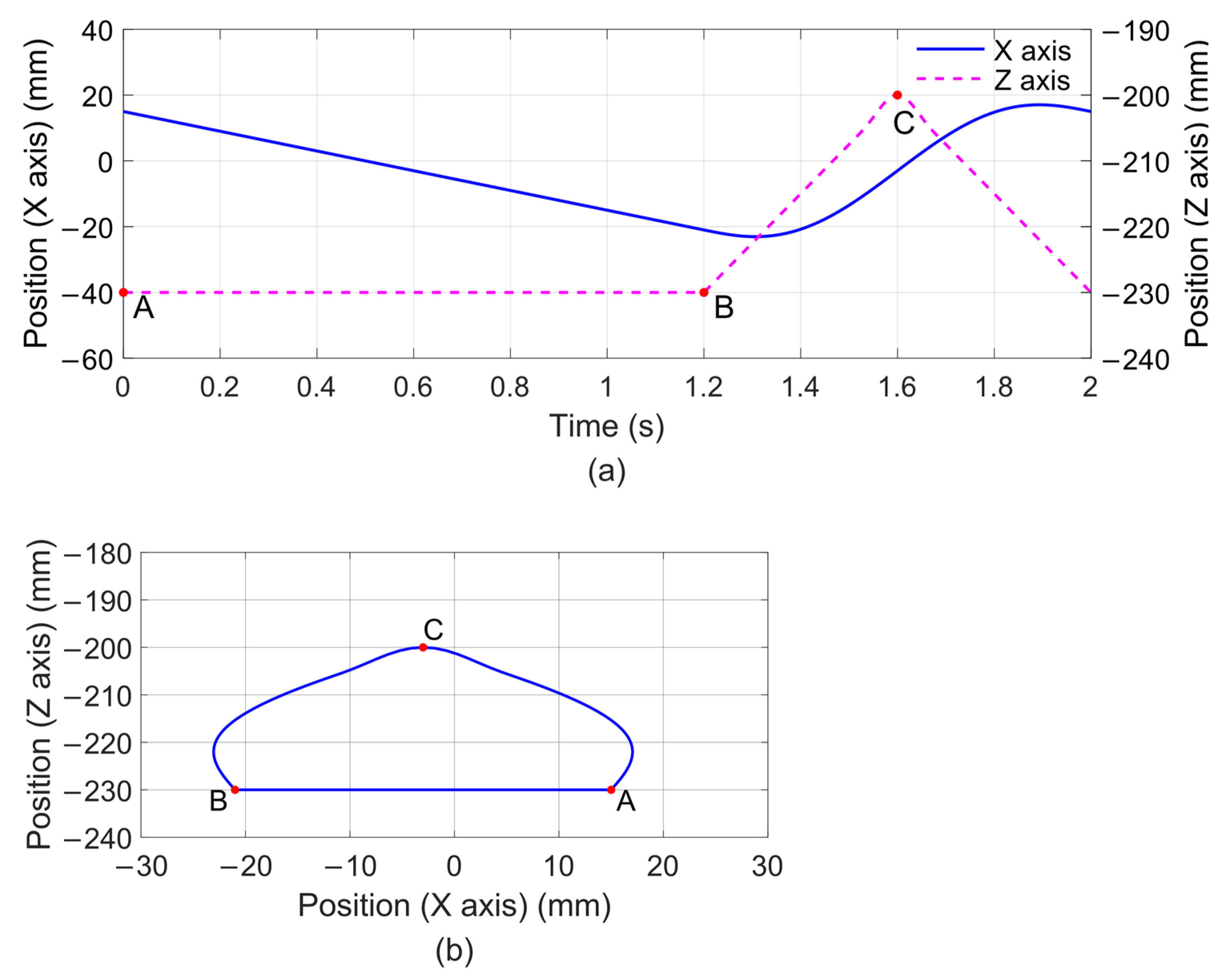
In the process of motion, some legs of the robot are in the state of swinging while other legs are in the state of supporting. The purpose of foot trajectory planning is to determine the complete foot trajectory of the leg in the process of swinging or supporting, which is important for the robot’s smooth movement [29]. In this paper, the foot trajectory of the leg i is planned relative to the coordinate frame {OiB} (i = 1~6). For straight gait, the foot position in the Y direction is always 0, so it only needs to plan the foot trajectory in the X and Z directions. This paper uses the polynomial fitting curve to plan the foot trajectory. It can be conveniently solved according to the constraints of foot position, velocity, and acceleration at the initial and end time [30], and it is also conducive to avoid the impact. Figure 4 shows an example of foot trajectory planning, which is a common situation in the straight gait of the robot. Three points A, B, and C are marked on the foot trajectory in the Z direction. When , the leg is in the support phase, matching the trajectory between “AB”. When the leg in the support phase, the actual foot position is unchanged. According to the relativity of motion, the foot trajectory in the X direction is planned as a straight line, which can better ensure to help the robot move forward at a constant speed. When , the leg is in the swing phase, matching the trajectory between “BCA”.
4. Straight Gait Planning
4.1. Increase of the Duty Factor
The main periodic gaits of the hexapod robot include the tripod gait, quadrangular gait, and pentagonal gait. In the tripod gait, three legs can swing at the same time, while two legs can swing at the same time in the quadrangular gait, and only one leg can swing at a time in the pentagonal gait. In this paper, when the robot starts to move until at least one leg moves from the swing phase to the support phase, it is considered that the robot has completed one “step”. In a cycle, all legs are required to complete a change in the swing phase and support phase. Therefore, each cycle of the triangular gait contains two steps, while the quadrangular gait and pentagonal gait, contains three and six steps, respectively.
Duty factor () is the time fraction of a cycle time when a particular leg is in the support phase [31]. Duty factor can be expressed as:
where is the total time of a cycle; and are the time that a particular leg is in the support phase and the swing phase in a cycle, respectively. In most of the previous gait planning schemes of hexapod robots, there is no case that six legs support the ground simultaneously in the gait cycle. For a single leg, it will only swing in one step in a cycle, while it will be in the support phase in other steps. Thus, the duty factors of the tripod gait, quadrangular gait, and pentagonal gait are 1/2, 2/3, and 5/6 respectively. can also be expressed as:
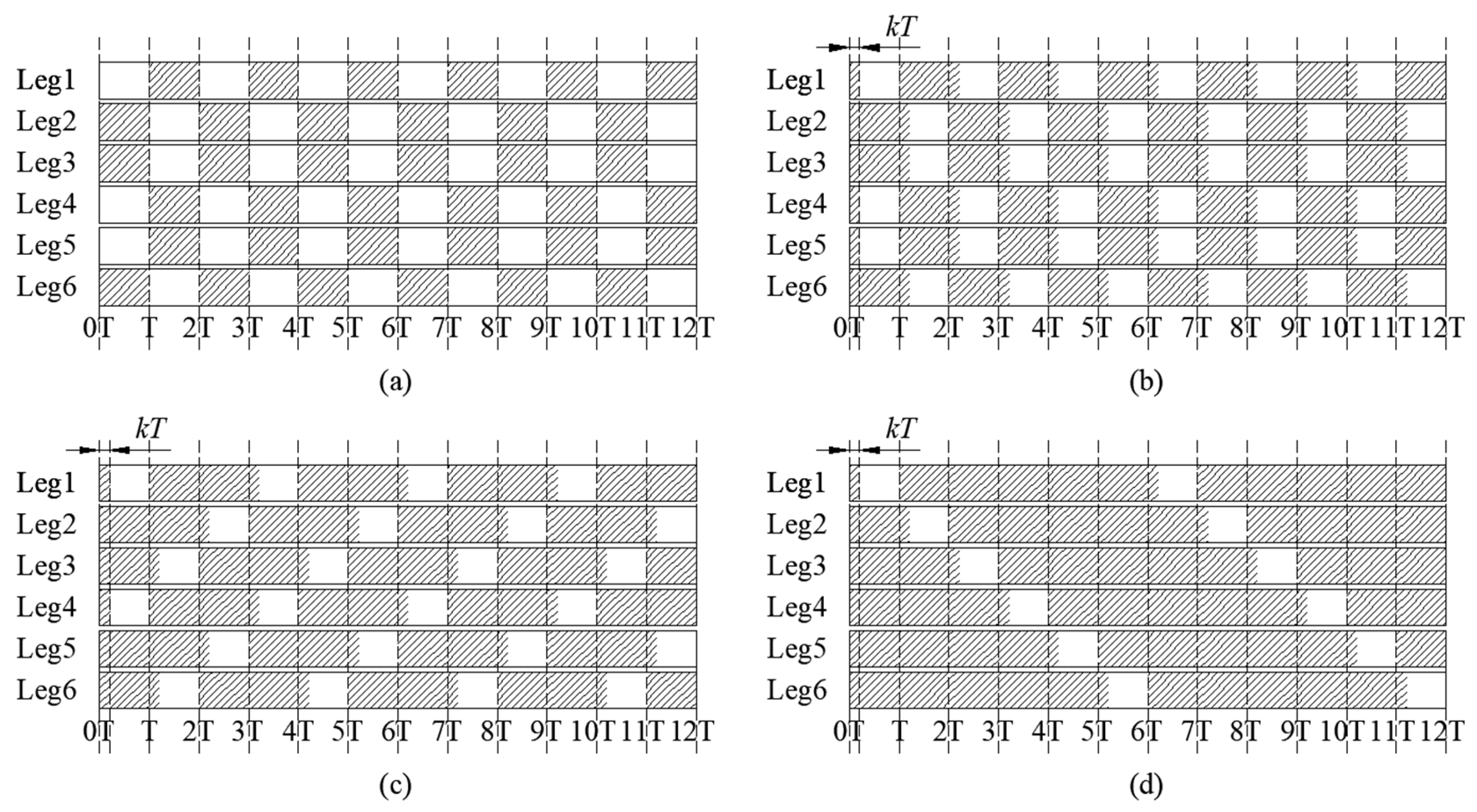
where T is the total time of each step; is a quantity, which represents that the single leg is completely in the support phase during steps in a walking cycle. The time sequence diagram of the robot walking forward in the general tripod gait is shown in Figure 5a [32]. The part of the shadow indicates that the leg is in the support phase, while the white part means the swing phase.
This paper puts forward the strategy of “increasing duty factor”, which aims to reduce foot slip and attitude fluctuation when the swing phase and the support phase switch. There is the stage where all six legs are in the support phase in each step. In each step, according to the previous gait planning, if a leg turns to be in the swing phase, it will not swing immediately, but is still in the support phase in the front kT (k is a factor between 0 and 1), supporting the body to move with other legs that are in the stance phase. The leg will swing in the next , and finally, make the foot swing to the planned position at the end of the step. Figure 5b–d depicts the time sequence diagram of the three gaits according to this strategy.
Based on this strategy, the duty factor becomes:
is determined by the gait type, while k can be set by trial according to the actual situation. Of course, k should not be set too large. It needs to leave enough swing time for the leg in one step. In the experiments of this paper, k is set to 0.2, so that the duty factors of tripod gait, quadrangular gait, and pentagonal gait become 3/5, 11/15, and 13/15.
4.2. Description Based on Discretization and Time Sequence Diagram
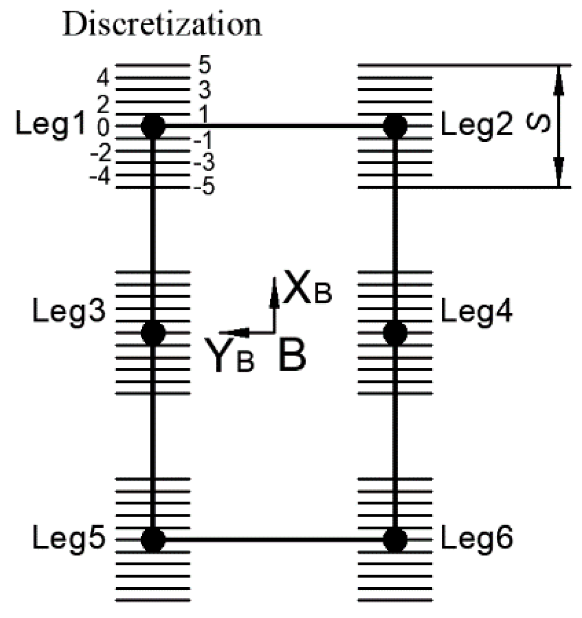
In this paper, a method based on the discretization and time sequence diagram is proposed, which can easily describe the straight gait of the hexapod robot. Gait discretization is an effective way to implement biological gait precisely [33]. Suppose S is the distance that the leg will support the body to move forward when it is in the support phase in each cycle. Discrete points can be used to describe support positions [34]. Now S is divided into 10 equal parts in Figure 6, and 11 integers of −5 to 5 are used to correspond to the beginning and end positions of each small distance, which represents the foot positions that can be selected at the beginning and end of each step.
If the discrete point corresponding to the foot position of the leg i is ( is an integer between −5 and 5), the foot position of the leg i under {OiB} can be easily drawn:
where H represents the current height of the body relative to the ground. Suppose that changes from to over a period of time. When the robot is moving forward, if , it can be known that leg i swings, and if , leg i has supported the body to move forward. The distance the foot moves can be expressed as .
Based on the discrete point, this paper defines the set {, , , , , } to represent the foot position state of the robot’s six legs. For the initial state, the robot is crouching, and {0, 0, 0, 0, 0, 0} can be used to describe the foot positions of the robot at this time.
Next, combining with the time sequence diagram, determine the foot positions of the robot at the beginning and end of each step, and intuitively describe the change process of the foot positions under all kinds of straight gaits.
Referring to Figure 5b, for tripod gait, a cycle contains two foot position states: {−5, 5, 5, −5, −5, 5} and {5, −5, −5, 5, 5, −5}. In a cycle (such as 0T~2T), when the robot walks forward using the tripod gait, the change in foot positions can be expressed as →→, as shown in Figure 7. represents the foot position state of the robot at T, while can represent the foot position state at 0T and 2T. Each cycle of the tripod gait includes two steps. Firstly, leg 2, leg 3, and leg 6 are used as supporting legs to support the body to move forward for the distance S. At the same time, leg 1, leg 4, and leg 5 swing forward from behind and move forward relative to the body. In the second step, the swing and support state of the two groups of legs are interchanged, and the robot advances the distance S again. All of the information can be obtained from the expression “→→”.
Referring to Figure 5c, for the quadrangular gait, a cycle contains three foot position states: {−5, 5, 0, −5, 5, 0}, {5, 0, −5, 5, 0, −5}, and {0, −5, 5, 0, −5, 5}. In a cycle (such as 0T~3T), when the robot walks forward using the quadrangular gait, the change in foot positions can be conveniently expressed as →→→. In each step, the body moves S/2.
Similarly, for the pentagonal gait, a cycle contains six foot position states: {−5, −3, −1, 1, 3, 5}, {5, −5, −3, −1, 1, 3}, {3, 5, −5, −3, −1, 1}, {1, 3, 5, −5, −3, −1}, {−1, 1, 3, 5, −5, −3} and {−3, −1, 1, 3, 5, −5}. In a cycle (such as 0T~6T), when the robot walks forward using the pentagonal gait, the change in foot positions is →→→→→→. In each step, the body moves S/5.
When the robot retreats, there is no need to redesign the change process of foot positions in each gait. The changing direction of the foot position state during the backward process is opposite to that of the forward. This time, in each step, the support leg supports the body to move backward, while the swing leg swings from front to back. For example, when the robot walks backward using the quadrangular gait, the change in foot positions is →→→.
4.3. Gait Transformation Scheme
In the beginning, the robot is crouching and needs a transformation to make it enter a certain gait cycle. Similarly, when the robot completes a specified number of cycles of motion, it can also transfer to the initial state to accept new instructions, to wait for new motion commands. What’s more, when the robot is moving using a certain gait, it may receive commands to change to walk by using other types of gait. Therefore, it is necessary to further design the online gait transformation planning that supports remote control.
The gait transformation scheme designed in this paper is based on the adjustment of foot positions. If the robot receives the command to change the gait during the motion, it will stop after completing the current step. The robot can then adjust the foot positions to a new state to enter the new gait cycle. There are two principles put forward for the adjustment of foot positions:
- Stability principle: When determining the swing leg, the robot should first be able to maintain static stability. Take leg 1, leg 4, and leg 5 as one group, and leg 2, leg 3, and leg 6 as another group. In one step, the robot can swing at most three legs at a time (the three legs must be in the same group), and the two adjacent legs cannot swing at the same time. Otherwise, the robot will lose its stability;
- Rapidity principle: On the premise of ensuring the stability of the robot, choose the least number of steps to adjust, then strive to adjust the least number of legs.
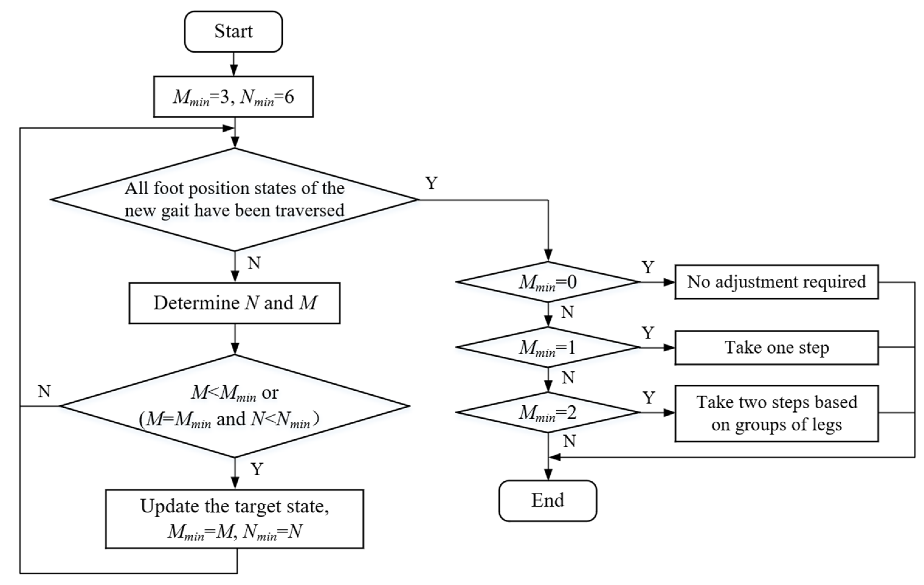
According to these two principles, Figure 8 shows the flow chart of gait transformation. Details are as follows:
- First, define a few parameters. M: the number of adjustment steps in gait transformation. N: the number of legs that need to be adjusted in gait transformation. Mmin: the minimum number of adjustment steps required in gait transformation. Nmin: the minimum number of legs required to be adjusted in gait transformation. The initial values of Mmin and Nmin are set to 3 and 6, respectively;
- Traverse each foot position state in the new gait and compare it with the current foot position state of the robot. The previous parameters can be determined in this process. Since the foot positions of the six legs are already included in the set P, when the two states are compared, N is easy to determine. Next, based on the stability principle, discuss in several situations: (1) If N is greater than 3, M must be 2; (2) If N is 3 and the three legs to be adjusted are in the same group, M is 1, otherwise M is 2; (3) If N is 2, and the two legs to be adjusted are not adjacent, M is 1, otherwise M is 2; (4) If N is 1, M is 1; (5) If N is 0, M is 0. This way, M can be determined. If M is less than Mmin, or although M is equal to Mmin, N is less than Nmin, update Mmin and Nmin, and make the current traversed foot position state as the target state;
- After the traversal is completed, the final adjustment steps can be determined. If Mmin is 0, the robot can directly enter the new gait without adjusting foot positions. If Mmin is 1, the robot only needs one step to complete the adjustment. If Mmin is 2, based on the grouping of robot legs in the tripod gait, we can only adjust the positions of the legs in the same group in one step to ensure the stability principle. And the gait transformation process is completed in two steps finally.
Here are two examples to illustrate the gait transformation scheme proposed in this paper. Consider a situation in which the robot changes from the tripod gait to the quadrangular gait. When the robot stops from the tripod gait, the foot position is assumed to be {5, −5, −5, 5, 5, −5} (). According to the gait transformation scheme, the target state can be determined as {5, 0, −5, 5, 0, −5} (). The robot only needs to adjust the foot positions of leg 2 and leg 5. When the two legs swing at the same time, the stability of the robot can be ensured, so only one step is needed to complete the transformation (). Then, consider another case in which the robot changes from the tripod gait to the pentagonal gait. When the robot stops, the foot position is also assumed to be {5, −5, −5, 5, 5, −5} (). The target state is {5, −5, −3, −1, 1, 3} (). At least four legs should be adjusted, which are leg 3, leg 4, leg 5, and leg 6. Mmin is now 2. Since leg 3 and leg 6 are in a group, they can swing at the same time. However, leg 4 and leg 5 need to swing in the second step. The whole gait transition process can be expressed as: →{5, −5, −3, 5, 5, 3}→.
5. Correction Algorithm of Yaw Angle
Based on the previous work, the basic motion control of the hexapod robot can be realized. The user can send instructions through the mobile device to make the robot realize the expected gait. Of course, this is just an open-loop control. Next, the actual feedback attitude information is used to design an algorithm to reduce the yaw of the robot’s attitude in motion.
The idea of the algorithm is to adjust the direction of the robot by adjusting foot positions of the support leg relative to the body coordinate system {B}, so that the robot can move close to the desired direction at the next moment to achieve the purpose of correcting the yaw angle in time. This way, when the robot determines the foot positions at the next moment, it needs to consider the adjustment of the walking direction, which is necessary to establish a kinematic model to describe it better. Figure 9 shows the kinematic model of yaw angle correction, here taking the tripod gait as an example. Suppose that the robot is not in the ideal direction at the current time, and the support leg needs the body to advance a distance of in the next moment ( can be determined based on the results of the original gait planning and foot trajectory planning). Now, to reduce the yaw angle error, make the robot rotate at an angle around the origin of the body coordinate system {B} to adjust to the ideal direction first. After that, the support legs can support the body forward.
Now it is necessary to recalculate and determine the foot position of each support leg relative to the coordinate frame {B} in the next moment. For the support leg i, suppose the foot position of it relative to {B} is at the current moment and at the next moment. Based on the kinematic analysis, the relationship between the two can be obtained:
Furthermore, we have
The foot position of the support leg i relative to {O1B} in the next moment can be further obtained. In this way, when the robot continues to move, the adjustment of the walking direction is added.
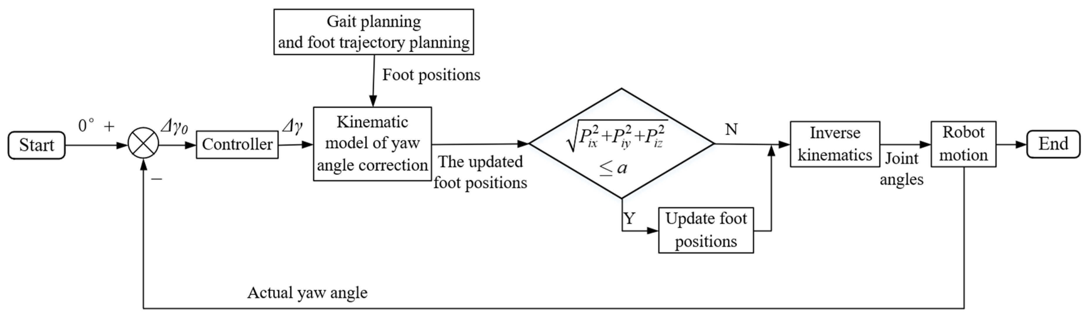
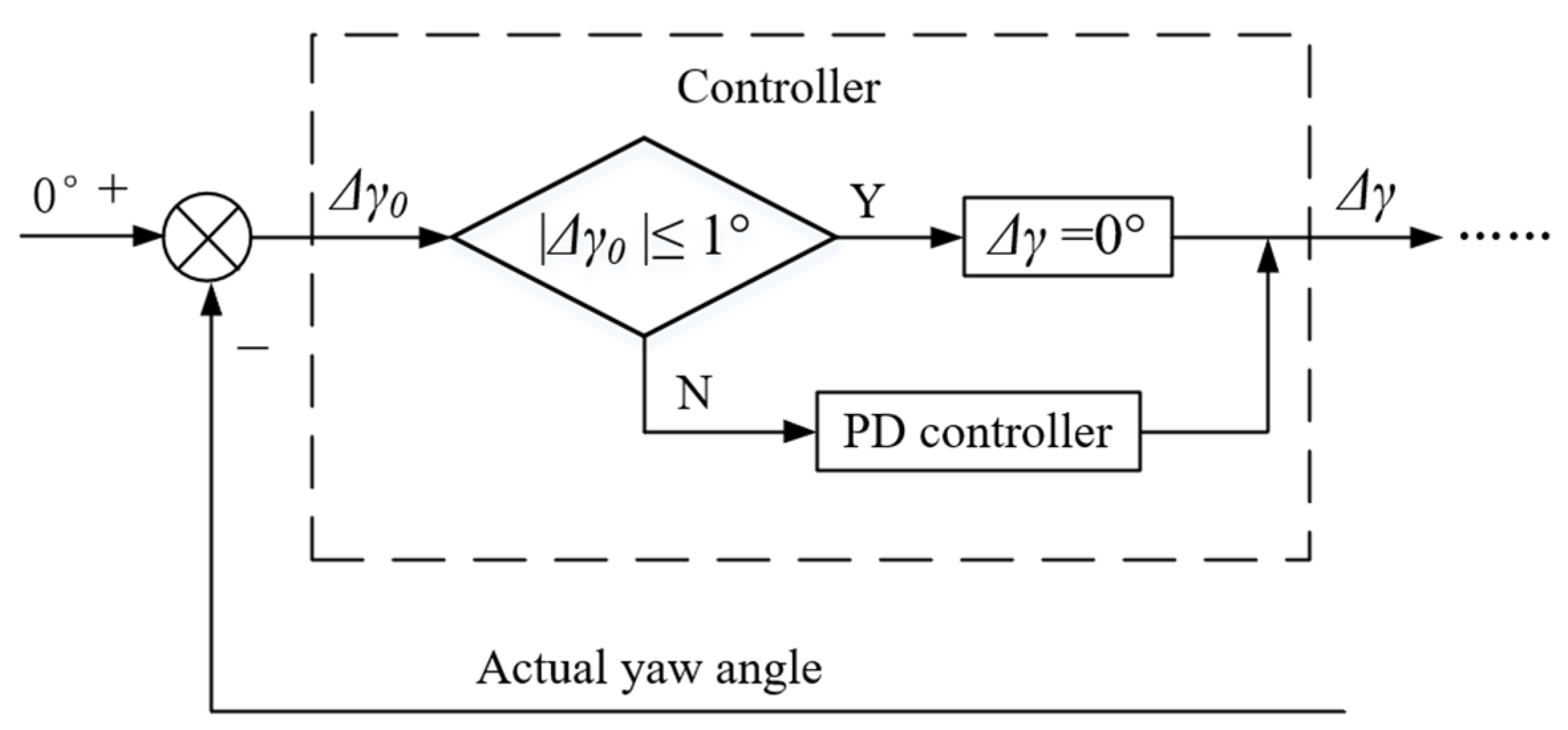
The flow chart of the yaw angle correction algorithm designed in this paper is shown in Figure 10.
In the straight gait, the desired yaw angle of the robot is always 0°. In the process of robot walking, the feedback information of yaw angle can be obtained based on the IMU module. Compared with the expected yaw angle, the difference is obtained as the input of the controller, and the output of the controller is , which is the variable in the previously proposed kinematics model of yaw angle correction for the robot. In the program, sampling is done every 10 ms.
According to the model, the foot positions of the robot’s support legs at each moment can then be recalculated to adjust the walking direction (See Equation (10)). After that, it needs to be judged whether the foot positions are within the maximum motion space range at this time. Suppose that the foot position of the leg i relative to {OiB} is , and use a to represent the total length of the robot leg. It is known that needs to be satisfied. If the foot position is not in the reachable motion space, it will not be updated, but still keep the value of the foot position at the previous time. Finally, according to the foot positions and the results of inverse kinematics analysis, the corresponding joint angles of the legs can be obtained, and then the servos can be driven to make the robot realize the specified motion.
The design of the controller is the key to the algorithm in Figure 10, and its internal form is shown in Figure 11. The design of the controller is the key of the algorithm, and its internal form is shown in Figure 11. The controller first makes a judgment. If is less than the threshold value (set to 1°), it is considered that the current actual yaw angle is acceptable, and the walking direction is not adjusted (directly output ). Otherwise, the PD controller is used to output . The PD controller is a kind of PID controller, which is simple in principle and easy to design. It can reduce the control error, accelerate the response speed of the system, and ensure robustness, which means it is not sensitive to the change in the environment and the parameters of the controlled object [35]. In the control program of the robot, an incremental PID algorithm is used to realize the PD controller. Each increment of can be calculated by where is the proportional coefficient; is the differential coefficient; and e(k) is the input deviation of the controller in the k-th sampling.
6. Experiments
Many experiments were done to verify the feasibility and effectiveness of the robot control algorithm and gait planning scheme. Next, some specific results are illustrated. In the experiments, the parameters of the robot are , , and . Here, as before, H stands for the height of the body, and T stands for the total time of each step, and S is the distance that a leg supports the robot to move for when it is in the support phase in a cycle.
6.1. Verification of Yaw Angle Control Algorithm
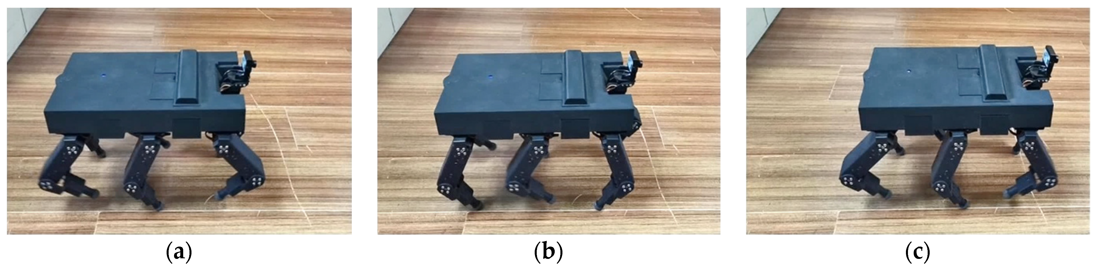
Figure 12 shows the experiment of HexWalker II walking forward using the tripod gait.
The first experiment completed is the tripod gait experiment of the robot without using the yaw angle correction algorithm. It can be known that when the robot is in the cycles of tripod gait normally, the time of a cycle is 2 s, and the ideal moving speed of the robot is . In 0 s~2 s, the robot is crouching, while it completes the adjustment of foot positions in 2 s~4 s. In 4 s~20 s, the robot walks forward for eight cycles using the tripod gait, and then after experiencing the adjustment of the foot positions again, it returns to the initial state. Based on the actual back reading data of each joint angle and the forward kinematics analysis of the robot, we can obtain the actual computational foot trajectory of each leg and compare it with the ideal planning foot trajectory to verify whether the robot can achieve the desired motion. Taking leg 1 as an example, the comparison between the ideal foot trajectory and the actual computational foot trajectory is shown in Figure 13. It is clear that the robot can achieve the expected motion.
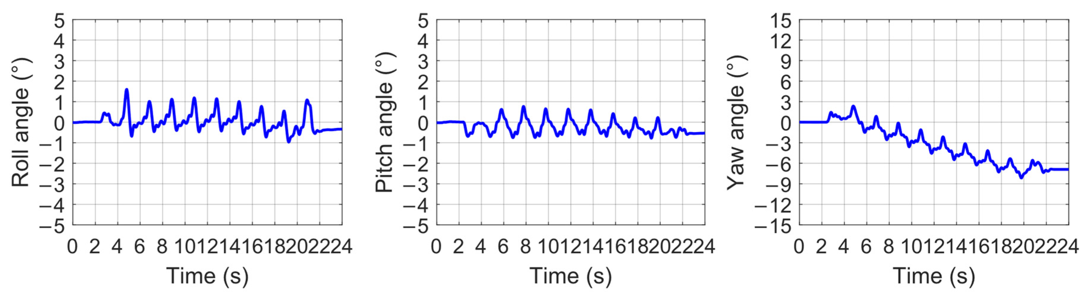
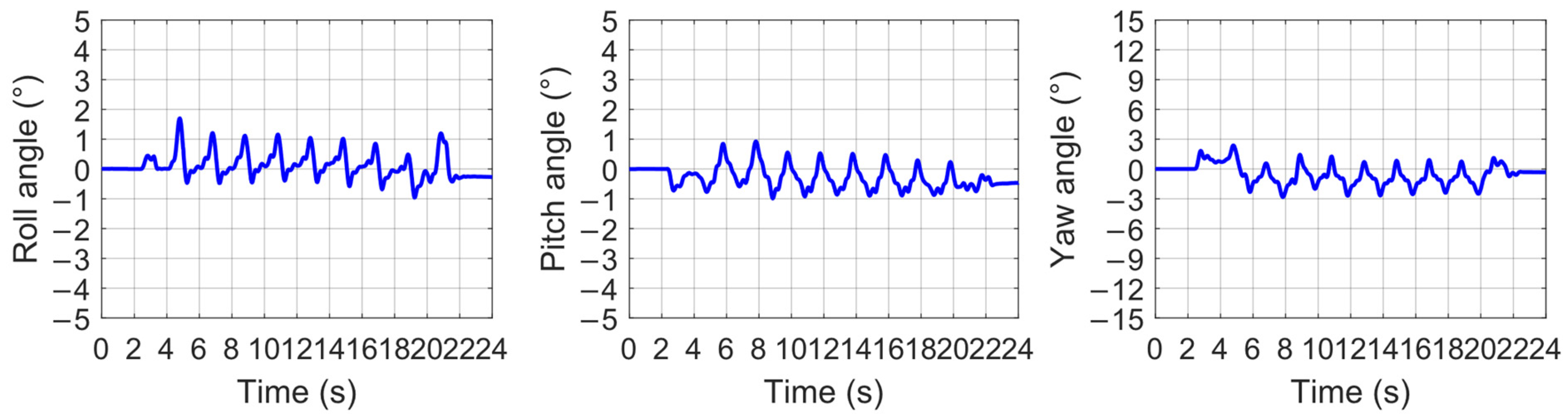
A group of attitude angle data when the robot walks forward using the tripod gait is shown in Figure 14. The orientation of the IMU module installation is consistent with that of the body coordinate frame {B} in Figure 3. The roll angle and pitch angle reflect the fluctuation of the robot body plane relative to the horizontal plane in the motion. According to the experimental data, the fluctuation amplitude is small, indicating that the robot’s motion is relatively stable. However, after eight cycles of motion, the yaw angle is close to −6°. There are many reasons for this phenomenon, including the change in the body’s center of gravity, mechanical error, impact and slip at the foot end, etc. Therefore, it is necessary to correct the yaw angle during the motion.
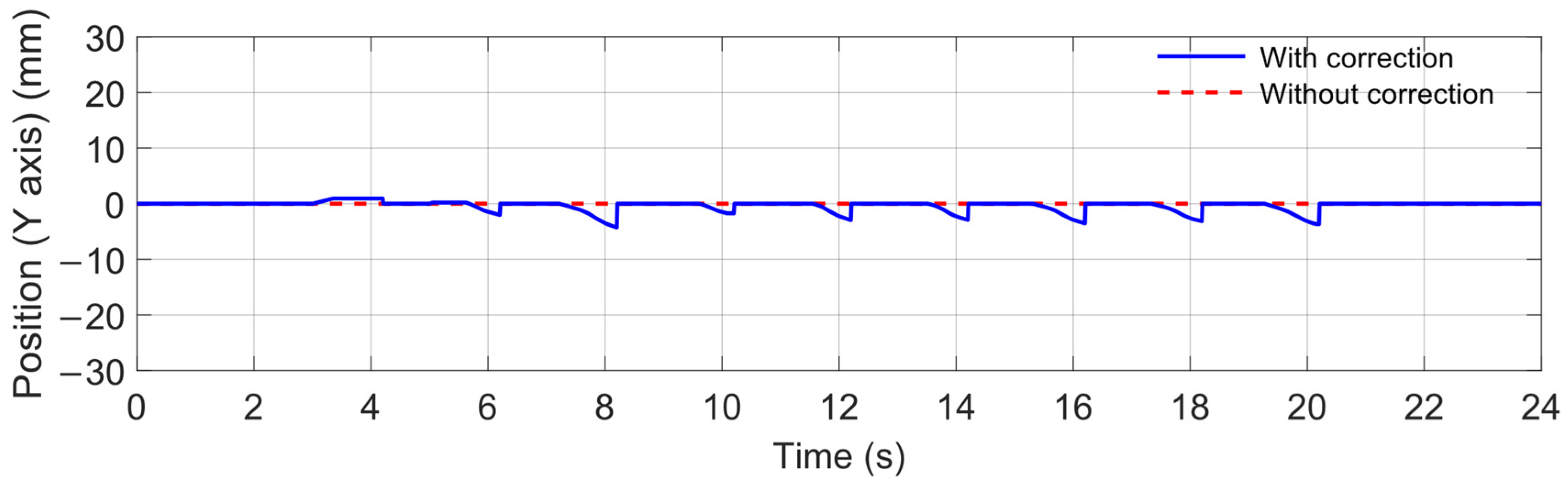
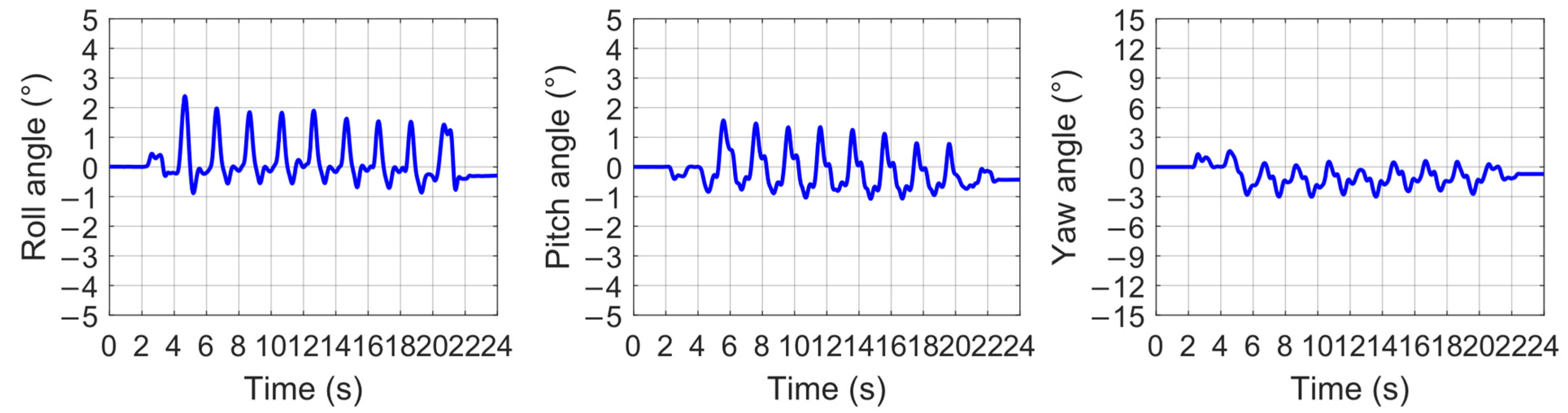
Other conditions remain unchanged, the previously designed yaw angle correction strategy is used in this experiment. Through trials, the parameters of the PD controller in the algorithm are set as: and . Take the foot trajectory of leg 1 in Y direction as an example. As shown in Figure 15, it can be found that when the leg is in the support phase, the ideal foot trajectory has changed, which indicates that the yaw angle correction algorithm is working to adjust the walking direction of the robot. Figure 16 shows the attitude angle data of the robot at this time.
It can be seen that the yaw angle correction algorithm has played a good role. The robot can reduce the yaw angle error by adjusting the direction in time during the motion. Table 3 compares the mean, standard deviation (SD) and root mean square error (RMSE) relative to the ideal value (0°) of the yaw angle data in two experiments. In the subsequent experiments, the yaw angle correction strategy is adopted by default.
6.2. Verification of the Strategy of “Increasing Duty Factor”
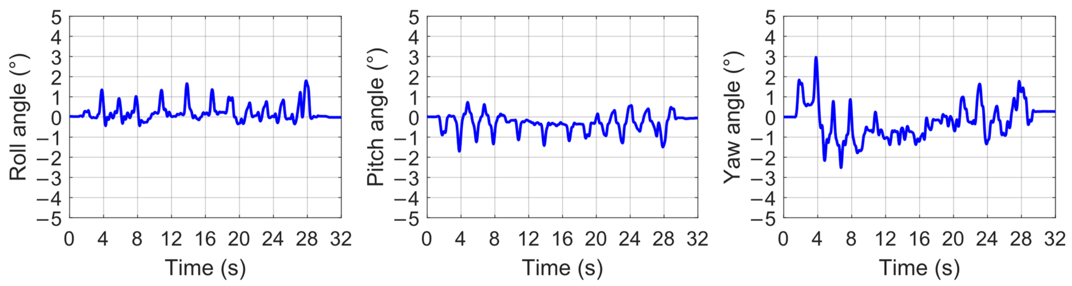
The gait planning of the robot adopts the previously designed strategy of “increasing duty factor”. In order to test its effect, this paper designs an experiment for comparison. In this experiment, the robot does not adopt that strategy, which means when a certain leg of the robot is about to enter the swing phase, it can immediately swing (the factor k is 0). The other conditions remain unchanged in the experiment, and the attitude angle data of the robot are shown in Figure 17. Compared with Figure 16, it can be found that the fluctuation degree of the attitude angle increases. The sampling time interval of attitude angle data is 10 ms. Table 4 compares the mean, SD, and RMSE of the attitude data in two experiments. The slipping degree of the robot’s foot is also more severe. In the experiment, after the robot completes 8 cycles of the tripod gait, the theoretical walking distance is 480 mm. Through measurement, in the previous experiment, the actual walking distance is about 460 mm, but it was only about 410 mm in this experiment.
6.3. Comparison and Transformation of Different Types of Gait
Three experiments are used to compare the results when the robot walks forward by using the tripod, quadrangular, and pentagonal gaits. In these three experiments, except for the different gait types, the other motion parameters are the same. The robot walks for 12 s using the tripod gait, 24 s using the quadrangular gait, and 60 s using the pentagonal gait. This way, for each gait, the theoretical walking distance is 360 mm. Table 5 shows the RMSE of the attitude angle data and the actual walking distance in the three experiments. From the tripod gait to the pentagonal gait, although the robot slows down, the attitude fluctuation and yaw also basically decrease, which means the stability of the robot’s motion is better. Since the quadrangular gait and the pentagonal gait require more steps, it may make the robot foot slip phenomenon more obvious to a certain extent, and increase the robot’s walking distance error [36]. Combing the actual needs, users can set suitable gait types and parameters on the mobile device.
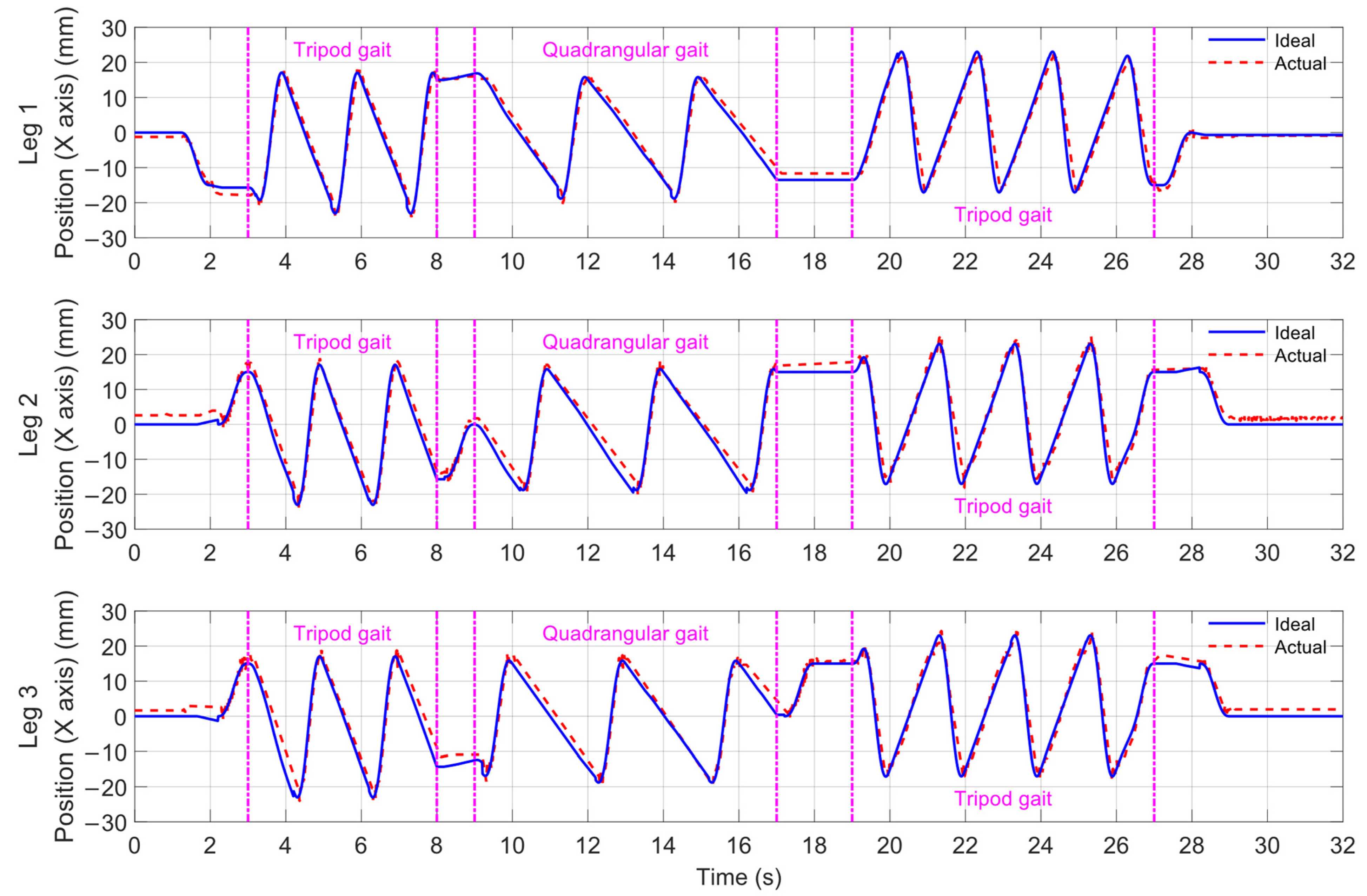
Figure 18 shows the foot trajectories of leg 1, leg 2, and leg 3 in the X direction in an experiment on gait transformation. Correspondingly, the attitude variations are shown in Figure 19. At first, the robot receives the command of walking forward using the tripod gait, but in the process of movement, it receives a command of walking forward using the quadrangular gait. After receiving the new command, the robot stops at 9 s. At this time, the foot positions of the robot’s legs can be expressed as {5, −5, −5, 5, 5, 5} (). To enter the cycles of quadrangular gait, the robot can adjust the foot positions by only one steps in situ: {5, −5, −5, 5, 5, −5} () → {5, 0, −5, 5, 0, −5} (), corresponding to 9 s~10 s. Then, the robot walks using the quadrangular gait and receives a command of walking backward using the tripod gait in 16 s~17 s. In 17 s~19 s, the robot completes two steps to adjust the foot position of three legs. The change process of foot positions is: {−5, 5, 0, −5, 5, 0} ()→{−5, 5, 5, −5, 5, 5}→{−5, 5, 5, −5, −5, 5} (). After that, the robot begins to walk backward for four cycles using the tripod gait, and finally returns to the initial state. The whole process conforms to the gait transformation scheme designed before.
7. Discussion and Conclusions
This paper designs a small electric hexapod robot called HexWalker II for daily life, which can be used in the fields of entertainment, education, monitoring, and so on. A set of gait planning schemes for the robot’s straight motion is made, including the realization of all kinds of basic gaits and the online transformation among them. The gait planning scheme is combined with our software on the mobile device and makes the robot respond to the instructions of users accurately and quickly on the premise of ensuring stability. In contrast to the traditional gait planning method, this paper proposes the strategy of “increasing duty factor”, which can reduce the posture fluctuation and foot end slip in robot motion. The experiment results show that the RMSE of the row, pitch, and yaw angle was reduced by 35%, 25%, and 12%, respectively, with this strategy. Based on the discretization and time sequence diagram, the straight gaits of the robot are described conveniently. According to the proposed principles of stability and rapidity, the detailed process of the robot gait conversion algorithm is also developed. In order to improve the reliability of robot motion, the kinematics model of robot yaw angle correction is constructed by using the attitude feedback information, and a yaw angle correction algorithm based on the PD controller is designed, which is easy to realize. The experimental results show that the drift of the yaw angle was suppressed effectively and was limited in the range −3°~3° using the control algorithm. The RMSE of the yaw data was reduced from 4.141° to 1.327° with the algorithm.
The gait planning schemes proposed in this paper are simple but effective. Compared to the traditional gaits, the “increasing duty factor” strategy can reduce the fluctuation of attitude, and the transformation process between different gait was described in detail. Compared to the posture control methods where Jacobian matrixes or foot forces are to be calculated, the yaw angle correction algorithm in this paper is easy to accomplish and calculate. The experiment results show that the drift of yaw angle can be effectively suppressed.
Although different kinds of gaits are studied in this paper, applications to the gait are lacking, such as transforming to a different gait according to the terrain, which could be studied in the future. Only the yaw angle was corrected during walking, which may not matter much when walking on flat ground, but to realize locomotion on uneven ground, the feedback and correction of all attitude angles will be needed.
Our current research is at a relatively initial stage. In the future, more gait planning schemes will be designed for the robot, such as turning and obstacle crossing, so that the robot can achieve more diverse forms of motion. At the same time, we will also make use of the existing sensor feedback of the robot, such as video images of the camera, to further design the closed-loop motion control algorithms to improve the robot’s motion performance and adaptability to the environment. Moreover, to improve the robustness of the gait motion, the feedforward control schemes could also be added [37], and some artificial intelligence approaches can be adopted to achieve the feedforward control methods [38]. We will then conduct more experiments to verify them.
Author Contributions
Conceptualization, F.Z., S.Z., Y.Y. and B.J.; methodology, F.Z., S.Z., Q.W. and B.J.; software, S.Z., Y.Y. and Q.W.; writing—original draft preparation, S.Z.; writing—review and editing, F.Z., S.Z. and B.J.; supervision F.Z. and B.J.; funding acquisition, B.J. All authors have read and agreed to the published version of the manuscript.
Funding
This work was supported by Ningbo Municipal Bureau of Science and Technology under Grant 2019B10052.
Conflicts of Interest
The authors declare no conflict of interest.
References
- Wan, G.; Deng, F.; Jiang, Z.; Lin, S.; Zhao, C.; Liu, B.; Chen, G.; Chen, S.; Cai, X.; Wang, H.; et al. Attention shifting during child—Robot interaction: A preliminary clinical study for children with autism spectrum disorder. Front. Inf. Technol. Electron. Eng. 2019, 20, 374–387. [Google Scholar] [CrossRef]
- Kanner, O.Y.; Rojas, N.; Odhner, L.U.; Dollar, A.M. Adaptive Legged Robots through Exactly Constrained and Non-Redundant Design. IEEE Access 2017, 5, 11131–11141. [Google Scholar] [CrossRef]
- Yang, Y. Fault-Tolerant Gait Planning for a Hexapod Robot Walking over Rough Terrain. J. Intell. Robot. Syst. 2009, 54, 613–627. [Google Scholar] [CrossRef]
- Xin, G.; Deng, H.; Zhong, G.; Wang, H. Gait and Trajectory Rolling Planning for Hexapod Robot in Complex Environment. In Mechanism and Machine Science; Springer: Singapore, 2017; pp. 23–33. [Google Scholar]
- Brooks, R.A. A Robot that Walks; Emergent Behaviors from a Carefully Evolved Network. Neural Comput. 1989, 1, 253–262. [Google Scholar] [CrossRef]
- Espenschied, K.S.; Quinn, R.D.; Beer, R.D.; Chiel, H.J. Biologically based distributed control and local reflexes improve rough terrain locomotion in a hexapod robot. Robot. Auton. Syst. 1996, 18, 59–64. [Google Scholar] [CrossRef]
- Chilian, A.; Hirschmüller, H.; Görner, M. Multisensor data fusion for robust pose estimation of a six-legged walking robot. In Proceedings of the 2011 IEEE/RSJ International Conference on Intelligent Robots and Systems, San Francisco, CA, USA, 25–30 September 2011; pp. 2497–2504. [Google Scholar]
- Zhang, H.; Liu, Y.; Zhao, J.; Chen, J.; Yan, J. Development of a bionic hexapod robot for walking on unstructured terrain. J. Bionic Eng. 2014, 11, 176–187. [Google Scholar] [CrossRef]
- Kim, J.; Jun, B.; Park, I. Six-legged walking of ‘Little Crabster’ on uneven terrain. Int. J. Precis. Eng. Manuf. 2017, 18, 509–518. [Google Scholar] [CrossRef]
- Kim, J.H.; Rhyu, S.H.; Jung, I.S.; Seo, J.M. An investigation on development of motor and gearheas for small mechanism. In Proceedings of the 2009 International Conference on Mechatronics and Automation, Changchun, China, 9–12 August 2009; pp. 1049–1053. [Google Scholar]
- Irawan, A.; Nonami, K. Optimal impedance control based on body inertia for a hydraulically driven hexapod robot walking on uneven and extremely soft terrain. J. Field Robot. 2011, 28, 690–713. [Google Scholar] [CrossRef]
- Davliakos, I.; Roditis, I.; Lika, K.; Breki, C.M.; Papadopoulos, E. Design, development, and control of a tough electrohydraulic hexapod robot for subsea operations. Adv. Robot. 2018, 32, 477–499. [Google Scholar] [CrossRef]
- Garcia, E.; Jimenez, M.A.; De Santos, P.G.; Armada, M. The evolution of robotics research. IEEE Robot. Autom. Mag. 2007, 14, 90–103. [Google Scholar] [CrossRef]
- Hwang, M.; Liu, F.; Yang, J.; Lin, Y. The Design and Building of a Hexapod Robot with Biomimetic Legs. Appl. Sci. 2019, 9, 2792. [Google Scholar] [CrossRef] [Green Version]
- Tedeschi, F.; Carbone, G. Design Issues for Hexapod Walking Robots. Robotics 2014, 3, 181–206. [Google Scholar] [CrossRef] [Green Version]
- Pratihar, D.K.; Deb, K.; Ghosh, A. Optimal path and gait generations simultaneously of a six-legged robot using a GA-fuzzy approach. Robot. Auton. Syst. 2002, 41, 1–20. [Google Scholar] [CrossRef]
- Collins, J.J.; Stewart, I. Hexapodal gaits and coupled nonlinear oscillator models. Biol. Cybern. 1993, 68, 287–298. [Google Scholar] [CrossRef]
- Cruse, H.; Kindermann, T.; Schumm, M.; Dean, J.; Schmitz, J. Walknet-a biologically inspired network to control six-legged walking. Neural Netw. 1998, 11, 1435–1447. [Google Scholar] [CrossRef]
- Görner, M.; Wimböck, T.; Hirzinger, G. The DLR Crawler: Evaluation of gaits and control of an actively compliant six-legged walking robot. Ind. Robot Int. J. 2009, 36, 344–351. [Google Scholar] [CrossRef]
- Pavone, M.; Arena, P.; Fortuna, L.; Frasca, M.; Patané, L. Climbing obstacle in bio-robots via CNN and adaptive attitude. Int. J. Circuit Theory Appl. 2006, 34, 109–125. [Google Scholar] [CrossRef]
- Chen, G.; Jin, B.; Chen, Y. Solving position-posture deviation problem of multi-legged walking robots with semi-round rigid feet by closed-loop control. J. Cent. South Univ. 2014, 21, 4133–4141. [Google Scholar] [CrossRef]
- Boscariol, P.; Henrey, M.A.; Li, Y.; Menon, C. Optimal Gait for Bioinspired Climbing Robots Using Dry Adhesion: A Quasi-Static Investigation. J. Bionic Eng. 2013, 10, 1–11. [Google Scholar] [CrossRef]
- Luneckas, M.; Luneckas, T.; Kriaučiūnas, J.; Udris, D.; Plonis, D.; Damaševičius, R.; Maskeliūnas, R. Hexapod Robot Gait Switching for Energy Consumption and Cost of Transport Management Using Heuristic Algorithms. Appl. Sci. 2021, 11, 1339. [Google Scholar] [CrossRef]
- Luneckas, M.; Luneckas, T.; Udris, D.; Plonis, D.; Maskeliunas, R.; Damasevicius, R. Energy-Efficient Walking over Irregular Terrain: A Case of Hexapod Robot. Metrol. Meas. Syst. 2019, 26, 645–660. [Google Scholar]
- Luneckas, M.; Luneckas, T.; Udris, D.; Plonis, D.; Maskeliūnas, R.; Damaševičius, R. A Hybrid Tactile Sensor-Based Obstacle Overcoming Method for Hexapod Walking Robots. Intel. Serv. Robot. 2021, 14, 9–24. [Google Scholar] [CrossRef]
- Zhai, S.; Jin, B.; Cheng, Y. Mechanical Design and Gait Optimization of Hydraulic Hexapod Robot Based on Energy Conservation. Appl. Sci. 2020, 10, 3884. [Google Scholar] [CrossRef]
- Xie, H.; Zhang, Z.; Shang, J.; Luo, Z. Mechanical Design of A Modular Quadruped Robot—Xdog. In Proceedings of the International Conference on Mechatronics, Electronic, Industrial and Control Engineering (MEIC 14), Shenyang, China, 15–17 November 2014; pp. 1074–1078. [Google Scholar]
- Corke, P.I. A Simple and Systematic Approach to Assigning Denavit-Hartenberg Parameters. IEEE Trans. Robot. 2007, 23, 590–594. [Google Scholar] [CrossRef] [Green Version]
- García-López, M.C.; Gorrostieta-Hurtado, E.; Vargas-Soto, J.E.; Ramos-Arreguin, J.M.; Sotomayor-Olmedo, A.; Morales, J.C. Kinematic analysis for trajectory generation in one leg of a hexapod robot. Procedia Technol. 2012, 3, 342–350. [Google Scholar] [CrossRef] [Green Version]
- Dau, V.; Chew, C.; Poo, A. Optimal trajectory generation for bipedal robots. In Proceedings of the 2007 7th IEEE-RAS International Conference on Humanoid Robots, Pittsburgh, PA, USA, 29 November–1 December 2007; pp. 603–608. [Google Scholar]
- Roy, S.S.; Pratihar, D.K. Effects of turning gait parameters on energy consumption and stability of a six-legged walking robot. Robot. Auton. Syst. 2012, 60, 72–82. [Google Scholar] [CrossRef]
- Sun, J.; Ren, J.; Jin, Y.; Wang, B.; Chen, D. Hexapod robot kinematics modeling and tripod gait design based on the foot end trajectory. In Proceedings of the 2017 IEEE International Conference on Robotics and Biomimetics (ROBIO), Macau, China, 5–8 December 2017; pp. 2611–2616. [Google Scholar]
- Li, M.; Zhang, X.; Zhang, J.; Zhang, M. Free gait generation based on discretization for a hexapod robot. In Proceedings of the 2013 IEEE International Conference on Robotics and Biomimetics (ROBIO), Shenzhen, China, 12–14 December 2013; pp. 2334–2338. [Google Scholar]
- Erden, M.S.; Leblebicioğlu, K. Free gait generation with reinforcement learning for a six-legged robot. Robot. Auton. Syst. 2008, 56, 199–212. [Google Scholar] [CrossRef]
- Tomei, P. Adaptive PD controller for robot manipulators. IEEE Trans. Robot. Autom. 2002, 7, 565–570. [Google Scholar] [CrossRef]
- Khalili, H.H.; Cheah, W.; Garcia-Nathan, T.B.; Carrasco, J.; Watson, S.; Lennox, B. Tuning and sensitivity analysis of a hexapod state estimator. Robot. Auton. Syst. 2020, 129, 1–17. [Google Scholar] [CrossRef]
- Cheng, X.; Tu, X.; Zhou, Y.; Zhou, R. Active Disturbance Rejection Control of Multi-Joint Industrial Robots Based on Dynamic Feedforward. Electronics 2019, 8, 591. [Google Scholar] [CrossRef] [Green Version]
- Reinhart, R.F.; Shareef, Z.; Steil, J.J. Hybrid Analytical and Data-Driven Modeling for Feed-Forward Robot Control†. Sensors 2017, 17, 311. [Google Scholar] [CrossRef] [PubMed]
Figure 1.
Picture of HexWalker II.

Figure 2.
Main contents of the motion control algorithm.

Figure 3.
D–H coordinate frames of HexWalker II.

Figure 4.
Foot trajectory relative to {OiB}: (a) Position variations in the X and Z directions; (b) Foot trajectory in the XZ plane.
Figure 4.
Foot trajectory relative to {OiB}: (a) Position variations in the X and Z directions; (b) Foot trajectory in the XZ plane.

Figure 5.
Time sequence diagram of the robot walking forward in tripod gait: (a) The general tripod gait; (b) The tripod gait with “increasing duty factor”; (c) The quadrangular gait with “increasing duty factor”; (d) The pentagonal gait with “increasing duty factor”.
Figure 5.
Time sequence diagram of the robot walking forward in tripod gait: (a) The general tripod gait; (b) The tripod gait with “increasing duty factor”; (c) The quadrangular gait with “increasing duty factor”; (d) The pentagonal gait with “increasing duty factor”.

Figure 6.
Discretization of foot positions on the ground.

Figure 7.
Walking forward using tripod gait.

Figure 8.
Flow chart of gait transformation.

Figure 9.
Kinematic model of yaw angle correction in straight gait.

Figure 10.
Flow chart of hexapod robot yaw angle correction algorithm.

Figure 11.
Controller design of hexapod robot yaw angle correction algorithm.

Figure 12.
The experiment of HexWalker II walking forward using tripod gait: (a) Leg 2, leg 3, and leg 6 are swinging; (b) Leg 1, leg 4, and leg 5 are swinging; (c) Leg 2, leg 3, and leg 6 are swinging.
Figure 12.
The experiment of HexWalker II walking forward using tripod gait: (a) Leg 2, leg 3, and leg 6 are swinging; (b) Leg 1, leg 4, and leg 5 are swinging; (c) Leg 2, leg 3, and leg 6 are swinging.

Figure 13.
Comparison between the ideal foot trajectory and the actual foot trajectory of leg 1 in tripod gait.
Figure 13.
Comparison between the ideal foot trajectory and the actual foot trajectory of leg 1 in tripod gait.

Figure 14.
Attitude variations in tripod gait (no correction).

Figure 15.
Comparison of ideal foot trajectory in Y direction of leg 1 with and without correction.

Figure 16.
Attitude variations in tripod gait (with correction).

Figure 17.
Attitude variations in tripod gait (without the strategy of “increasing duty factor”).

Figure 18.
Comparison between the ideal foot trajectory and the actual foot trajectory of leg 1~3 in the experiment of gait transformation.
Figure 18.
Comparison between the ideal foot trajectory and the actual foot trajectory of leg 1~3 in the experiment of gait transformation.

Figure 19.
Attitude variations in the experiment of gait transformation.


Table 1.
D–H parameters for the HexWalker II’s leg.
| Link | ||||
|---|---|---|---|---|
| 1 | 0 | −90° | ||
| 2 | 0 | 0 | ||
| 3 | 0 | 0 |
Table 2.
Actual values of D–H parameters.
| Range | Length | ||
|---|---|---|---|
| [−20°, 20°] | 42 mm | ||
| [−85°, 85°] | 100 mm | ||
| [−85°, 85°] | 100 mm |
Table 3.
Comparison of data in two experiments.
| Data Type | Data in the Experiment with the Algorithm | Data in the Experiment without the Algorithm |
|---|---|---|
| The mean of the yaw data | −0.804° | −3.323° |
| The SD of the yaw data | 1.056° | 2.472° |
| The RMSE of the yaw data | 1.327° | 4.141° |
Table 4.
Comparison of data in two experiments.
| Data Type | Data in the Experiment with the Strategy | Data in the Experiment without the Strategy |
|---|---|---|
| The mean of the roll data | 0.156° | 0.205° |
| The mean of the pitch data | −0.263° | −0.118° |
| The mean of the yaw data | −0.804° | −1.127° |
| The SD of the roll data | 0.453° | 0.710° |
| The SD of the pitch data | 0.428° | 0.659° |
| The SD of the yaw data | 1.056° | 1.011° |
| The RMSE of the roll data | 0.479° | 0.739° |
| The RMSE of the pitch data | 0.502° | 0.669° |
| The RMSE of the yaw data | 1.327° | 1.514° |
Table 5.
Comparison of data in three experiments.
| Data Type | Experimental Data of Tripod Gait | Experimental Data of Quadrangular Gait | Experimental Data of Pentagonal Gait |
|---|---|---|---|
| The mean of the roll data | −0.063° | 0.060° | 0.121° |
| The mean of the pitch data | −0.091° | −0.009° | −0.178° |
| The mean of the yaw data | −0.840° | −0.837° | −0.525° |
| The SD of the roll data | 0.385° | 0.398° | 0.236° |
| The SD of the pitch data | 0.355° | 0.290° | 0.221° |
| The SD of the yaw data | 0.900° | 0.368° | 0.296° |
| The RMSE of the roll data | 0.390° | 0.403° | 0.265° |
| The RMSE of the pitch data | 0.366° | 0.290° | 0.284° |
| The RMSE of the yaw data | 1.231° | 0.914° | 0.603° |
| The actual walking distance | 345 mm | 335 mm | 324 mm |
Publisher’s Note: MDPI stays neutral with regard to jurisdictional claims in published maps and institutional affiliations. |
© 2021 by the authors. Licensee MDPI, Basel, Switzerland. This article is an open access article distributed under the terms and conditions of the Creative Commons Attribution (CC BY) license (https://creativecommons.org/licenses/by/4.0/).
Share and Cite
MDPI and ACS Style
Zhang, F.; Zhang, S.; Wang, Q.; Yang, Y.; Jin, B. Straight Gait Research of a Small Electric Hexapod Robot. Appl. Sci. 2021, 11, 3714. https://0-doi-org.brum.beds.ac.uk/10.3390/app11083714
AMA Style
Zhang F, Zhang S, Wang Q, Yang Y, Jin B. Straight Gait Research of a Small Electric Hexapod Robot. Applied Sciences. 2021; 11(8):3714. https://0-doi-org.brum.beds.ac.uk/10.3390/app11083714
Chicago/Turabian StyleZhang, Feng, Shidong Zhang, Qian Wang, Yujie Yang, and Bo Jin. 2021. "Straight Gait Research of a Small Electric Hexapod Robot" Applied Sciences 11, no. 8: 3714. https://0-doi-org.brum.beds.ac.uk/10.3390/app11083714
Note that from the first issue of 2016, this journal uses article numbers instead of page numbers. See further details here.