Target Recovery for Robust Deep Learning-Based Person Following in Mobile Robots: Online Trajectory Prediction

Abstract

The ability to predict a person’s trajectory and recover a target person in the event the target moves out of the field of view of the robot’s camera is an important requirement for mobile robots designed to follow a specific person in the workspace. This paper describes an extended work of an online learning framework for trajectory prediction and recovery, integrated with a deep learning-based person-following system. The proposed framework first detects and tracks persons in real time using the single-shot multibox detector deep neural network. It then estimates the real-world positions of the persons by using a point cloud and identifies the target person to be followed by extracting the clothes color using the hue-saturation-value model. The framework allows the robot to learn online the target trajectory prediction according to the historical path of the target person. The global and local path planners create robot trajectories that follow the target while avoiding static and dynamic obstacles, all of which are elaborately designed in the state machine control. We conducted intensive experiments in a realistic environment with multiple people and sharp corners behind which the target person may quickly disappear. The experimental results demonstrated the effectiveness and practicability of the proposed framework in the given environment.

1. Introduction

Mobile robots that accompany people may soon become popular devices similar to smartphones in every day life with their increasing use in personal and public service tasks across different environments such as homes, airports, hotels, markets, and hospitals [1]. With the growing number of intelligent human presence detection techniques and autonomous systems in various working environments, the abilities of such systems to understand, perceive, and anticipate human behaviors have become increasingly important. In particular, predicting the future positions of humans and online path planning that considers such trajectory predictions are critical for advanced video surveillance, intelligent autonomous vehicles, and robotics systems [2]. Recent advances in artificial intelligence techniques and computing capability have allowed a high level of understanding comparable to that of humans in certain applications. The employment of these advances in robotic systems to enable the completion of more intelligent tasks is an interesting development [3].

To robustly follow a specific person to a destination position in realistic narrow environments including many corners, the robots must be able to efficiently track the target person. Many challenges arise in a variety of scenarios when the person moves out of the field of view (FoV) of the camera when the person turns a corner, becomes occluded by other objects, or makes a sudden change in her/his movement. This disappearance may lead the robot to stop and wait in its location until the target person returns to the robot’s FoV. Unfortunately, such situations may be unacceptable for the users. The robot must be therefore able to predict the trajectory of the target person to recover from such failure scenarios. This is a significant challenge. Accurate distance estimation, localization, and safe navigation with obstacle avoidance present additional challenges for the robotic follower system. A further important consideration is the ability of the robot to switch smoothly between state machine control without the freezing robot problem (FRP) [4], which was presented in [5] as a big limitation. Intuitively, the FRP happens when the robots believe the environment to be unsafe, i.e., every path is expected to collide with an obstacle due to massive uncertainty [6].

In this paper, we proposed a novel target recovery method for a mobile robot to seamlessly follow a target person to a destination using online trajectory prediction. This was achieved by integrating a recovery mode based on the person-following framework developed in our previous work [7]. The person-following framework performs many necessary cognitive tasks such as human detection and tracking, person identification, distance estimation between the robot and people, target trajectory prediction, mapping, localization, online path planning, navigation, and obstacle avoidance. Furthermore, it seamlessly integrates the algorithms, the Robot Operating System (ROS) processes, and various sensor data. This integration improves the ability of the mobile robot to handle unexpected scenarios. The proposed system also addresses the aforementioned challenges and provides a more intelligent algorithm for person-following robots.

The contributions made in this paper can be summarized as follows: First, we present a novel method for a robot to recover to the tracking state when the target person disappears, by predicting the target’s future path based on the past trajectory and planning the robot’s movement path accordingly. Second, we integrated a recovery method based on a deep learning-based person-following system into a robotic framework. Third, we present an efficient and seamless state machine control scheme that works selectively based on the robot state to maintain the robot in an active state while following the person. Fourth, we demonstrate the proposed recovery with intensive experiments in realistic scenarios.

The rest of this paper is organized as follows: Some related works are presented in Section 2. In Section 3, we briefly explain the proposed framework and its main parts. The experimental settings and the obtained results are presented in Section 4. We conclude the paper and outline future works in Section 5.

2. Related Work

In this section, we provide a brief overview of previous works on person-following robots and target person trajectory prediction. One of the earliest person-following robot techniques reported in 1998 integrated a color-based method and a sophisticated contour-based method to track a person using a camera [8]. Subsequent works studied robots that follow the target from behind using a visual sensor [9] or 2D laser scanners [10], a robot that accompanies the person side-by-side using a LiDAR sensor [11], and a robot that acts as a leader in airports to guide passengers from their arrival gate to passport control [12].

Robotics and computer vision are fields in which technological improvements emerge every day. Several tracking methods for mobile robots based on various sensing sensors for people and obstacle detection have been reported. These methods include the use of 2D laser scanners in indoor environments [13] and in both indoor and outdoor environments [10]. Range finders provide a wide FoV for human detection and tracking [11]. However, such range sensors provide poor information for people detection compared to visual sensors. RGB-D cameras such as Orbbec Astra [7] and Kinect [14] are visual sensors that have been adopted in recent years and are currently available on the market. These cameras are suitable for indoor environments, easy to use on robots, and provide synchronized depth and color images in real time. In this study, we used an Orbbec Astra RGB-d camera to track the people and the LiDAR sensor to detect obstacles and navigate when the target is lost.

Several human-following robot systems have been proposed in different outdoor or indoor environments in recent years. However, there have been a few attempts to address the target recovery from a failure situation using the online trajectory prediction. Calisi et al. [15] used a pre-trained appearance model to detect and track a person. If the person is lost, the robot continues to navigate to the last observed position (LOP) of the target person and then rotates 360° until it finds the person again. However, the recovery task fails if the robot cannot find the person after reaching the LOP and completing the 360° rotation. Koide and Miura [16] proposed a specific person detection method for mobile robots in indoor and outdoor environments in which the robot moves toward the LOP continuously if it loses the target. Our previous work [7] adopted a deep learning technique for tracking persons, used a color feature to identify the target person, and navigation to the LOP, then a random searching to recover the person if he/she is completely lost. Misu and Miura [17] used two 3D LiDAR sensors together with AdaBoost and a Kalman filter to generate points could for people detection in outdoor environments. To recover the target, they used two electronically steerable passive array radiator (ESPAR) antennas as a receiver and a transmitter to estimate the position of the target, then started the searching operations. However, this method has poor accuracy for human detection. Chen et al. [18] proposed an approach based on an online convolutional neural network to detect and track the target person. They used trajectory replication-based techniques to recover missing targets. However, the aforementioned systems used simple methods to recover the target person, such as navigation to the LOP, random searching, or rotation. These methods usually fail if the target is not nearby the LOP or take a long time to recover the target compared to the methods, which predict a target’s trajectory.

Ota et al. [19] developed a recovery function based on a logarithmic function. However, this method is not compatible with environments involving multiple people. Hoang et al. [20] adopted Euclidean clustering and histogram of oriented gradient (HOG) features with a support vector machine (SVM) classifier to detect the legs of persons. They used a probabilistic model (Kalman filter) and map information (width of the lobby), which allowed the robots to grasp the searching route in order to recover the target in an indoor environment. Although the target always had one direction to turn behind the corner and the robot took a long time to recover the target, i.e., from the 42th frame to the 1175th frame, it failed in 20% of the experiments. These approaches were developed when deep learning techniques were not yet common and cannot perform robust human detection.

Unlike previous methods, Lee et al. [21] adopted a deep learning technique called you only look once (YOLO) for tracking people in real time and applied a sparse regression model called variational Bayesian linear regression (VBLR) for trajectory prediction to recover a missing target. However, this method has a high computational cost despite the use of a GPU.

3. System Design of Mobile Robot Person-Following System

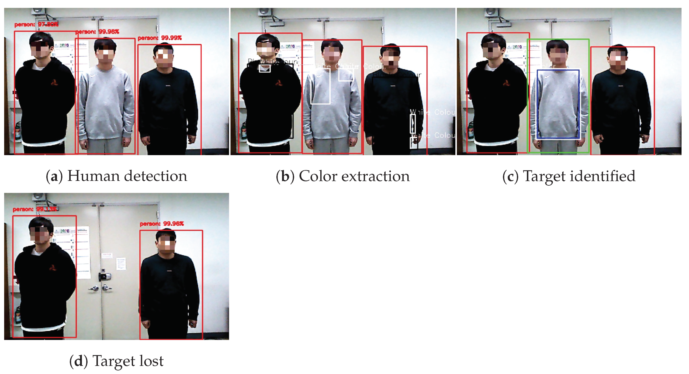
In this paper, we proposed a novel recovery function using online trajectory prediction that extends our previous human-following framework [7] so that a mobile robot can more seamlessly follow the target person to the destination. The overall framework, including person tracking, identification, and trajectory prediction, is illustrated in Figure 1. In detail, the framework primarily consists of the following parts: (1) human detection and tracking, (2) depth information and position estimation, (3) person identification, (4) target trajectory prediction, (5) path planners, and (6) the robot controller including target recovery. In the human detection and tracking part, persons are detected and tracked by the single-shot multibox detector (SSD) deep neural network technique using the 2D image sequences from the camera on the robot. The SSD is pre-trained and used in this study as explained in [22]. The position estimation module estimates the poses of people in the real-world space rather than in the image space using point clouds [23]. In the person identification module, the target person is identified based on the color of his/her clothes by using the hue-saturation-value (HSV) model to extract the color feature. In the target trajectory prediction part, which was designed to utilize the path history of the target, we adopted the best algorithm by comparing the person-following performances of the robot across various algorithms. For online path planning, we used adaptive Monte Carlo localization (AMCL) [24] to accurately localize the position of the robot. The robotic controller was designed to follow the target person continuously along a course in a pre-built 2D map created from depth laser data using a simultaneous localization and mapping (SLAM) algorithm. If the robot loses the target person, it recovers him/her via state machine control using the predicted target trajectory. We adopted three techniques from our previous work [7], namely the SSD detector, the HSV model, and the position estimation module, in addition to the two controllers for the LOP and the searching states. Figure 2 shows the image processing steps in the workflow. The SSD model first detects humans with confidence scores (Figure 2a); then, the clothing color is extracted (Figure 2b) for identifying the target person and other persons (Figure 2c). When the target disappears from the camera’s FoV (Figure 2d), the robot attempts to recover him/her again to the tracking state. The green bounding box around a person indicates the target person, and the red bounding boxes indicate the other people. The blue rectangle on the target person indicates the region of interest (ROI), and the white rectangles indicate the detection of the clothes’ colors. In the following subsections, we describe these parts in more detail.

In this study, we used a mobile robot called Rabbot made by Gaitech. The robot is shown in Figure 3. The weight of the robot is 20 kg, and it is designed to carry approximately 50 kg. The robot is equipped with various sensors such as an Orbbec Astra RGB-d camera and a SLAMTEC RPLiDAR A2M8. The on-board main controller of the robot uses a computer with a hex-core, 2.8 GHz, 4 GHz turbo frequency i5 processor, 8 GB RAM, and 120 GB SSD running Ubuntu 16.04 64-bit and ROS Kinetic. The camera was installed 1.47 m above the floor for better visual tracking of the scene.

The computing performance of vision processing was critical for smooth and robust person-following in this study. In order to keep the frames per second (FPS) as high as possible, we ran the vision processing on a separate workstation (Intel Core i7-6700 CPU @ 3.40 GHz). In the distributed computing environment, the workstation (Node 1) and the on-board computer on the robot (Node 2) communicate with each other and simultaneously share sensor data including the 2D image sequences as needed. Node 1 is responsible for the human detection and tracking, position estimation, and person identification modules. Node 2 is responsible for the system controller, mapping, and target trajectory prediction modules. If the target person is tracked, Node 1 sends the most basic information of the target to Node 2 as a publisher, which receives this information as a subscriber. Otherwise, Node 1 sends a signal to inform the system controller that the target is lost. The basic communication between the nodes is accomplished using the ROS framework [25]. The wireless connection between the two nodes is established using the 802.11ac WiFi network, which provides a sufficiently stable connection within the environment described in the Results and Discussion Section later.

3.1. Human Detection and Tracking

Many algorithms for the localization of objects in the scene have been developed in recent years. These algorithms, which include Faster R-CNN (regions with CNN) [26], the SSD [22], and YOLO [27], have high detection accuracy and efficiency in using 2D bounding boxes to detect objects. The algorithms predict the most likely class for each region, generate bounding boxes around possible objects, and discard regions with low probability scores. However, they require pre-trained datasets. The SSD achieves a better balance between speed and accuracy compared to its counterparts. It is faster than Faster R-CNN and more accurate than YOLO [22]. We implemented the comparison in terms of the speed for the three algorithms on our workstation using the CPU. Faster R-CNN, YOLO, and the SSD achieved real-time performance at 1.40, 2.50, and 25.03 fps using the CUP, respectively. The performance may change if a GPU is available.

With our objective of obtaining a high frame rate, we ultimately adopted the SSD detector to distinguish people from other objects using the MobileNets database [7]. The details of the SSD are beyond the scope of this paper, so we only briefly describe the SSD here. The SSD is a detector based on a fully convolutional neural network consisting of different layers that produce feature maps with multiple scales and aspect ratios. A non-maximum suppression method is then implemented to detect objects of different sizes using bounding boxes and to generate the confidence scores as an output, as shown in Figure 2a. The SSD requires only a sequence of $300\times 300$ 2D color images as the input to a single feed-forward process. The vertices of the bounding boxes and the centers of these boxes relative to the whole image resolution are given in the formats of ($u_{max},u_{min},v_{max},v_{min}$) and $c_u=((u_{max}-u_{min})/2)$, $c_v=((v_{max}-v_{min})/2)$, respectively.

3.2. Position Estimation Using Depth Information

The distance is recorded in the path history of the target so that the trajectory of the person can be predicted when the person is lost. To facilitate the estimation of distances from the RGB-D data, we converted the coordinates from 2D to 3D using the point cloud after determining the centers of the people in 2D images ($(c_{u_i},c_{v_i})$) and the camera point. Consider the detection of many people $P_i$, $i=1,2,3,\dots ,n$ by the robot. The relationship between the 3D coordinates of a person $(X_i,Y_i,Z_i)$ and the center of the boundary box of the person in the 2D RGB image coordinates $(c_{u_i},c_{v_i})$ is given by:

$$\left[\begin{array}{c}{c}_{u_i}\\ c_{v_i}\\ 1\end{array}\right]=\left[\begin{array}{ccc}{f}_x& s& u_0\\ 0& f_y& v_0\\ 0& 0& 1\end{array}\right]\left[\begin{array}{c}{X}_i\\ Y_i\\ Z_i\end{array}\right]$$

(1)

where ($u_0$, $v_0$) is the center point of the image, $f_x$ and $f_y$ are the focal lengths along each axis in pixels, and s is an axis skew that arises when the u and the v axes are not perpendicular. Once all of these parameters are known, the distance $d_i$ between the person and the center point of the camera in meters can be estimated using the following equation:

$$d_i=\sqrt{X_i^2+Y_i^2+Z_i^2}.$$

(2)

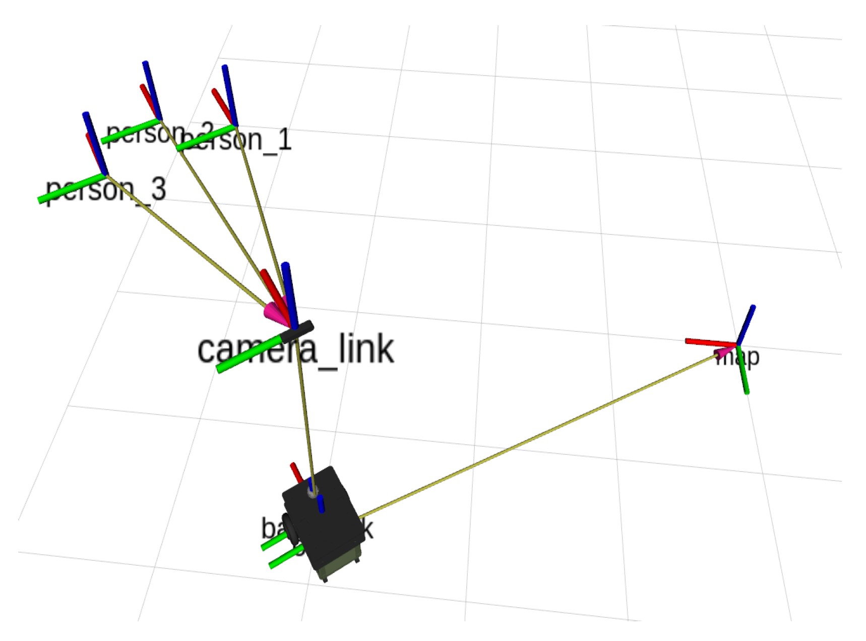
We adopted the transform library (tf) in [28] to transfer the 3D coordinates of the persons and join them with the SLAM algorithm and the coordinates of the rest of the system, as depicted in Figure 4.

The pose of the robot in 2D plane navigation is represented by only ($x_r,y_r,{\theta }_r$), where the angle ${\theta }_r$ indicates the heading direction. An Orbbec Astra camera was used to provide synchronized color and depth data at a resolution of $640\times 480$ over a ${60}^{\circ }$ horizontal field of view. The angles of the persons relative to the center of the camera are dependent on the camera specifications used and are computed as ${\phi }_i=-0.09375\times c_{u_i}+30$, where $c_{u_i}$ is the center of the box on the u axis. Then, from the previous equations, we obtain the real-world positions of the persons as:

$$\begin{array}{c}{x}_i=d_{i}cos\left({\theta }_r+{\phi }_i\right)+x_r\hfill \\ y_i=d_{i}sin\left({\theta }_r+{\phi }_i\right)+y_r.\hfill \end{array}$$

(3)

3.3. Person Identification

Many methods for identifying objects based on their texture, color, or both have been studied. These methods include HOG [29], scale-invariant feature transformation (SIFT) [30], and the HSV color space [31]. In this study, we adopted the HSV color space to extract the clothing color for identifying the target person, which is robust to illumination [32]. This color space was used effectively in an indoor environment under moderate illumination changes in our previous work [7]. HSV channels were applied to each of the ROIs for color segmentation to identify the color of the clothes. Segmentation is an important technique in computer vision, which reduces computational costs [33]. To extract the color feature in real time, the image color was filtered by converting the live image from the RGB color space to the HSV color space. Then, the colors of the clothes were detected by adjusting the HSV ranges to match the color of the target person. Next, morphological image processing techniques, such as dilation and erosion, were used to minimize the error and remove noise. Finally, the color of the clothes was detected in rectangular regions at different positions and areas determined according to the contours, as shown in Figure 2b. Invalid areas that were very small were filtered out using a minimum threshold value. As depicted in Figure 2c,d, once the person identification module identifies the target person, it sends the basic information of the person (position, angle, and area of the boundary box) to the control system, as described above.

3.4. Target Trajectory Prediction

Target trajectory prediction is quite a significant topic in robotics in general and is especially essential in person-following robot systems. The trajectory prediction algorithm predicts the future trajectory of the target, that is the future positions of the person over time, when the target is lost. In this paper, we present a novel approach to predict the trajectory of the target based on comparing the performance of various algorithms and selecting the algorithm with the best performance.

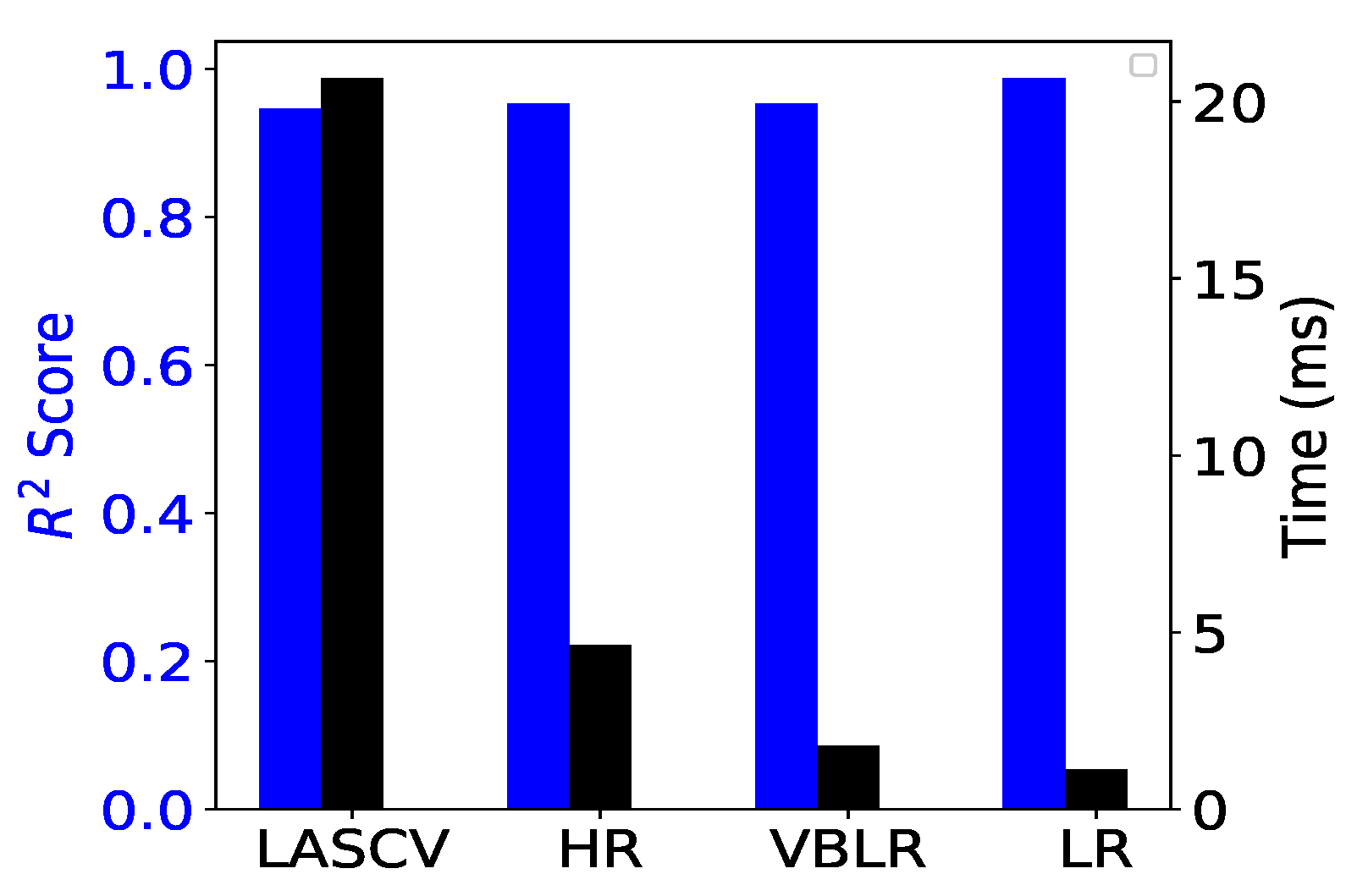
We compared a wide variety of regression models to determine the most appropriate model for online learning and predicting the trajectory data. We trained the Lasso cross-validation (LasCV), Huber regressor (HR), VBLR, and linear regression (LR) models by fitting the trajectory data obtained at the corners in the environment. The blue and black bars in Figure 5 indicate the $R^2$ scores for the accuracy and time for the computation time, respectively. Among the models with high accuracy, we chose the LR model, which is the fastest model, for our trajectory prediction. All the models were implemented using Scikit-learn [34], a powerful machine learning library [35].

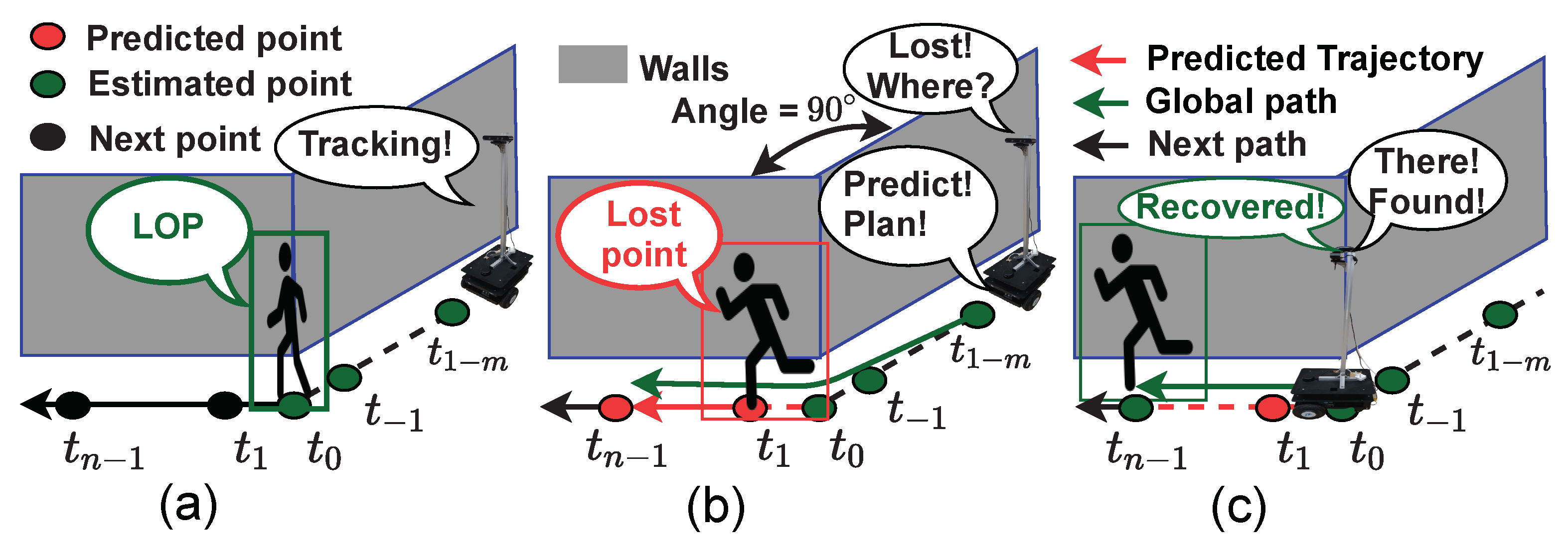
A scenario in which the target is lost and recovered by path prediction is shown in Figure 6. Figure 6a shows a person turning 90° at a corner and suddenly disappearing from the FoV of the robot. The person turns at the corner at $t_0$ (Figure 6a) and disappears from the FoV of the camera at $t_1$ (Figure 6b). The robot predicts the target’s trajectory and then plans the global and local planners to recover the tracking of the person at $t_{n-1}$ (Figure 6c). The trajectory prediction algorithms rely only on the stored past trajectory information. Therefore, the mobile robot estimates and stores the time series-based positions of the target person while tracking the target person using the RGB-D sensor. The training data $D_{tr}$ consist of m pairs of $(x,y)$ positions with their associated timestamps $t_k$:

$$D_{tr}=\left(\left(x_0,y_0\right),t_0\right),\dots ,\left(\left(x_{1-m},y_{1-m}\right),t_{1-m}\right)$$

(4)

where $t_k>t_{k-1}$ for $k=0,\dots ,1-m$. The input of the person positions along the x coordinate is $\mathbf{x}=x_{0:1-m}$; that along the y coordinate is $\mathbf{y}=y_{0:1-m}$; and the corresponding timestamps are $\mathbf{t}=t_{0:1-m}$.

We adopted the linear regression model in this work and then applied the second-order polynomial with a constrained output of one of the coordinates to predict the target trajectory using an online method. The approach consists of the following four steps: In the first step, the last 50 positions, which are empirically obtained and critical, are used only in the training module. Thus, $m=50$. These data are feed into the linear regression model as the input. In the second step, the relationship between the dependent variables $(x,y)$ and the independent variable $\left(t\right)$ is modeled. In simple linear regression, the model is described by:

$$\begin{array}{c}x=a_{1}t+b_1\hfill \\ y=a_{2}t+b_2.\hfill \end{array}$$

(5)

In the third step, a second-order polynomial is applied to predict the trajectory of the target as follows:

$$\begin{array}{c}x=a_1{t}^2+b_{1}t+c_1\hfill \\ y=a_2{t}^2+b_{2}t+c_2\hfill \end{array}$$

(6)

where $a_1$, $b_1$, $c_1$, $a_2$, $b_2$, and $c_2$ are arbitrary parameters that are estimated from the data. The linear regression model is transferred from a first-order model to a second-order one. This transformation is a common approach in machine learning for adopting trained linear models to nonlinear functions while retaining the speed of the linear methods. The model is still a linear regression model from the point of view of estimation [36]. In the fourth step, the output of one of the coordinates is constrained. The trajectory consists of m pairs of $(x,y)$ positions on the 2D plane. Its length can be bounded in the x coordinate by $\Delta x$ and in the y coordinate by $\Delta y$, which are given by:

$$\begin{array}{c}\Delta x=x_0-x_{1-m}\hfill \\ \Delta y=y_0-y_{1-m}.\hfill \end{array}$$

(7)

If $|\Delta x|>|\Delta y|$, the robot is considered to be following the target along the x coordinate regardless of the slope between the $x-y$ coordinates. Thus, only the output of the x coordinate is constrained while that of the y coordinate is not, as $x=x_{k=5}$ for $k\ge 5$, empirically obtained. The y coordinate is treated in a similar manner. If $|\Delta x|<|\Delta y|$, $y=y_{k=5}$ for $k\ge 5$. The trajectory prediction takes the form of the predicted data $D_{pr}$, which consist of n pairs of $(x,y)$ positions with their associated timestamps $t_k$, given by:

$$D_{pr}=\left(\left(x_0,y_0\right),t_0\right),\dots ,\left(\left(x_{n-1},y_{n-1}\right),t_{n-1}\right)$$

(8)

where $t_k<t_{k+1}$ for $k=0,\dots ,n-1$. The output of the person positions along the x coordinate is $\mathbf{x}=x_{0:n-1}$, and that along the y coordinate is $\mathbf{y}=y_{0:n-1}$ with the corresponding timestamps $\mathbf{t}=t_{0:n-1}$. $(n-1)$ represents the last predicted position (LPP) in the trajectory prediction and is equal to two times m, that is $n=2m=100$, which was obtained empirically. Finally, the robot predicts the target’s trajectory when the target disappears from the FoV of the camera. The main goal of the robot at which the robot tries to find the target is the LPP $(x_{n-1},y_{n-1})$. The LPP should fall within the boundaries of the known map. If the LPP is outside of the boundaries of the known map, the robot will move to its secondary goal, which is the nearest position from the boundaries. The movement of the robot involves the path planners, which are presented next.

3.5. Path Planner

Path planning in mobile robots is a key technology and is defined as finding a collision-free path connecting the current point and the goal point in the working environment. The advantages of path planning include minimizing the traveling time, the traveled distance, and the collision probability. The mobile robot should navigate efficiently and safely in highly dynamic environments to recover its target. The recovery procedure based on the output of the target trajectory prediction module is comprised of three steps. The first step is the target trajectory prediction, which was described above. The second step is the planning of the trajectory between the current position of the robot and the LPP by the global planner. This trajectory is shown as the green path in Figure 6b. The third step involves the local path planner. In this study, the default global planner was based on the move_base ROS node. The global path planner, which allows the robot to avoid static environmental obstacles, is executed before the mobile robot starts navigating toward the destination position. The local planner was based on the timed-elastic-band (TEB) planner in the ROS. To autonomously move the robot, the local path planner monitors incoming data from the LiDAR to avoid dynamic obstacles and chooses suitable angular and linear speeds for the mobile robot to traverse the current segment in the global path (Equation (10); see more details in [37,38]).

3.6. Robot Controller Including Target Recovery

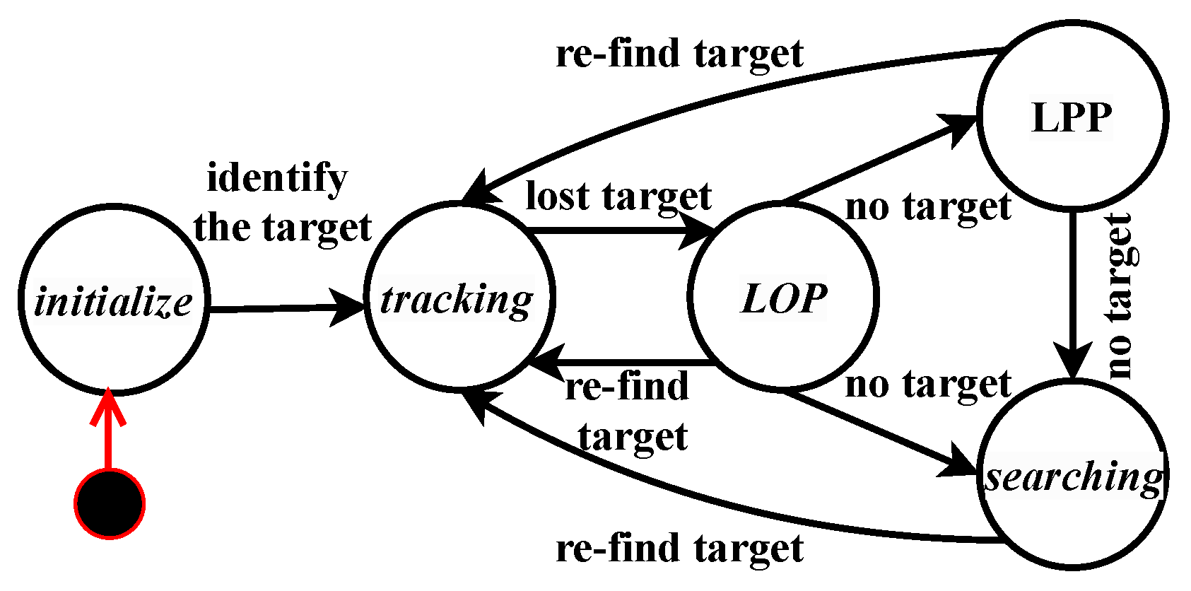
We defined four main states for controlling the mobile robot, that is namely, the tracking, LOP, LPP, and searching states, in addition to the initialization state, as shown in Figure 7. It is important to keep the target person in the FoV of the robot while executing the person-following task. The LOP, LPP, and searching states are called recovery states. In these states, the control module aims to maintain the robot in an active state for the recovery of a lost target using the LiDAR sensor. In the tracking state, the robot follows the target while tracking the target using a visual sensor. In the LOP state, the robot navigates to the last observed position of the target in the tracking state after the target has disappeared in the first attempt to recover the target. If the target cannot be recovered, the robot will switch to the LPP state in the second attempt. If the robot does not find the target at the LPP, it will switch to the searching state where it rotates and scans randomly in the final attempt.

In special cases, the robot switches from the LOP to the searching state if the last observed distance is less than one meter, that is if the target is very close to the robot.

Closed-loop control is implemented for all the states except the searching state. The linear velocity (V) and angular velocity $\left(\omega \right)$ of the robot in the three different control states are defined as follows:

$$\mathrm{Tracking}\mathrm{state:}\begin{array}{c}V=k_{tv}(0.5A-a)\hfill \\ \omega =k_{tw}{(320-c_u)}^2,\hfill \end{array}$$

(9)

$$\mathrm{LOP}\mathrm{state:}\begin{array}{c}V=k_{lv}\sqrt{{\left(y_t-y_r\right)}^2+{\left(x_t-x_r\right)}^2}\hfill \\ \omega =k_{lw}\left({\phi }_t-{\theta }_r\right),\hfill \end{array}$$

(10)

$$\mathrm{and}\mathrm{LPP}\mathrm{state:}\begin{array}{cc}\hfill V_k& \simeq \frac{1}{\Delta T_k}∥\left(\begin{array}{c}{x}_{k+1}-x_k\\ y_{k+1}-y_k\end{array}\right)∥\hfill \\ \hfill {\omega }_k& \simeq \frac{{\theta }_{k+1}-{\theta }_k}{\Delta T_k}.\hfill \end{array}$$

(11)

where $k_{tv}$, $k_{tw}$, $k_{lv}$, and $k_{lw}$ are constants with the values of $85\times {10}^{-7}$, $258.8\times {10}^{-7}$, 1, and 1, which are empirically obtained, respectively. A is a constant that represents the camera resolution of $640\times 480$, and a is the area of the target boundary box in a 2D image sequence in pixels. $c_u$ is the center of the target box on the u axis in pixels. In the tracking state, the robot moves forward if a is less than 0.5 A and backward otherwise. It turns right if $c_u$ is less than 320 and turns left otherwise. [$x_r,y_r,{\theta }_r$] and [$x_t,y_t,{\phi }_t$] represent the real-world poses of the robot and the target at the LOP moment (Figure 6a). In the LOP state, the robot first turns right if ${\theta }_r$ is less than ${\phi }_t$ and turns left otherwise. It then always moves forward to the LOP. ($x_{k+1}-x_k$), ($y_{k+1}-y_k$), and (${\theta }_{k+1}-{\theta }_k$) are the Euclidean and angular distances between two consecutive configurations $k,k+1$. $\Delta T_k$ is the time interval for the transition between the two poses. In the LPP state, the robot moves forward to its goal unless there are no dynamic obstacles in its path. If there are obstacles, the robot moves back to avoid a collision. It turns right if ${\theta }_k$ is less than ${\theta }_{k+1}$ and turns left otherwise (more details in [37,38]).

4. Results and Discussion

We performed intensive experiments to evaluate the proposed recovery framework for the mobile robot using online target trajectory prediction in a realistic scenario. In this section, we present and discuss the results of the experiments.

4.1. Experimental Setting

A realistic scenario for testing the target recovery in the experimental environment is depicted in Figure 8. The target person starts from inside Helper Lab (S) and walks about 25 m to the elevator (E) at the end of the corridor to the left. The narrow corridor is only two meters wide. The path includes two corners: Corner 1 and Corner 2. When the person turns at the corners, he/she may quickly disappear from the FoV of the camera (potentially in two directions).

The green and blue dashed paths represent the trajectories of the target person and the robot, respectively. The red circles denote the other persons, who are non-targets. The blue letters denote the glass windows, doors, walls, and the ends of the corridors. The white area denotes the known map and the gray area the unknown map. We used the 802.11ac WiFi network to have a wireless connection between the robot and the workstation, and it was stable enough within the environment to obtain the experimental results in this paper.

4.2. Experimental Results

Figure 9 shows the snapshots of the robot’s view in an experiment. The green and red rectangles around the persons indicate the target person and the other persons, respectively. The white rectangle on the target person represents the color detection, while the blue rectangle indicates the ROI on the target person. The ROI was used to ensure that the color was extracted only from the person’s clothes. The ROI is especially important in a colorful environment like ours, that is where there were black, white, green, yellow, orange, and blue scenes.

The robot started to follow its target from the laboratory to the end of the corridor based on the color feature in the indoor environment. Initially, the color feature was extracted and the distance of the target estimated simultaneously by the RGB-D camera. The system identified the target person wearing the white t-shirt as the target and another person who stood up in the middle of the laboratory as a non-target. Then, the robot started to follow the target person (Figure 9a). The robot continued to follow the person from the departure position toward the destination position. After a few seconds, the target turned left by approximately 90° at the first corner (Figure 9b). We call this moment the LOP (Figure 6a). The target suddenly disappeared from the FoV of the camera when he/she was in the corridor and the robot was still in the laboratory (Figure 9c). Over the duration at which the target disappeared, the robot correctly predicted his/her trajectory, planned the trajectory to recover the target, and resumed tracking the target (Figure 9d). The robot continued to follow the target and detected another person who stood up in the corridor as a non-target (Figure 9e). The target walked in an approximately straight line for a few meters, then turned right 90° at the second corner (Figure 9f). The target suddenly disappeared again from the FoV of the camera (Figure 9g). The robot correctly predicted the target’s trajectory and planned the recovery of the target to the tracking state at the destination position where the target arrived (Figure 9h). In this experiment, the mobile robot achieved continuous success in following the target person despite two sudden disappearances.

To assess the performance of the proposed system, we set two criteria for the success of the mission. The first criterion was whether the robot successfully followed the target person to the destination point. If the robot did not reach the destination point, we considered the experiment a failure, regardless of the causes of the failure or the percentage of the travel distance during the experiment. The second criterion was whether the robot correctly predicted the target’s future path trajectory after missing the target at the corners. In all the experiments, the velocities, coordinates, distances, and time were measured in meters per second, meters, meters, and seconds, respectively.

The results of the 10 experiments are summarized in

Table 1. Results of the experiments involving target recovery at the corners.

	Performance Measures	Exp.1	Exp.2	Exp.3	Exp.4	Exp.5	Exp.6	Exp.7	Exp.8	Exp.9	Exp.10	Total	Average	Std
Overall	Experiment success	O	O	O	O	O	O	O	X	O	O	90%	-	-
	Target’s travel distance (m)	24.4	23.9	25.0	24.9	23.5	24.1	23.6	15.0	23.8	23.6	231.7	23.2	2.92
	Robot’s travel distance (m)	22.0	22.8	22.2	22.3	22.1	22.0	22.4	14.2	22.2	22.0	214.3	21.4	2.56
	Robot’s travel time (s)	45.3	45.5	49.6	48.2	51.7	47.3	47.8	41.3	47.1	51.5	475.5	47.6	3.10
	Robot’s average velocity (m/s)	0.49	0.50	0.45	0.46	0.43	0.47	0.47	0.34	0.47	0.43	0.45	0.45	0.04
	No. of frames	1092	1143	1171	1220	1210	1149	1171	1025	1145	1245	11571	1157	64.09
	Successful tracking (frames)	730	697	687	595	722	811	800	738	756	766	7302	730	62.11
	Lost tracking (frames)	362	446	484	625	488	338	371	287	389	479	4269	427	97.50
	Successful tracking (s)	30.3	27.8	29.1	23.5	30.9	33.4	32.7	29.7	31.1	31.7	300.2	30.0	2.8
	Track lost (s)	15.0	17.8	20.5	24.7	20.9	13.9	15.1	11.6	16.0	19.8	175.3	17.5	3.9
	Lost tracking rate (%)	0.33	0.39	0.41	0.51	0.40	0.29	0.32	0.28	0.34	0.38	-	0.37	0.07
	Successful tracking rate (%)	0.67	0.61	0.59	0.49	0.60	0.71	0.68	0.72	0.66	0.62	-	0.63	0.07
	FPS	24.1	25.1	23.6	25.3	23.4	24.3	24.5	24.8	24.3	24.2	-	24.4	0.6
Corner 1	Trajectory prediction success	O	O	O	O	O	O	O	O	O	O	-	-	-
	Time when lost (s)	13.2	10.8	13.2	12.9	11.5	12.9	12.5	11.1	12.9	10.4	-	12.13	1.08
	Time when recovered (s)	18.4	15.7	19.0	19.9	18.9	18.0	18.0	15.8	17.6	15.2	-	17.66	1.59
	Recovery time (s)	5.2	4.9	5.9	7.0	7.4	5.1	5.5	4.7	4.7	4.8	-	5.52	0.98
	TDR when losing (m)	3.8	3.9	4.1	4.0	4.0	3.9	3.9	4.0	4.1	3.9	-	3.95	0.10
	TDR when recovering (m)	6.6	6.6	7.3	7.7	7.1	6.5	6.5	6.1	6.4	6.4	-	6.71	0.49
	Recovery distance (m)	2.8	2.7	3.1	3.7	3.2	2.6	2.6	2.1	2.4	2.4	-	2.76	0.48
	Recovery velocity (m/s)	0.54	0.54	0.54	0.53	0.43	0.52	0.48	0.44	0.50	0.50	-	0.50	0.04
Corner 2	Trajectory prediction success	O	O	O	O	O	O	O	N	O	O	-	-	-
	Time when lost (s)	32.3	30.7	33.2	38.7	34.1	34.8	35.0	-	32.1	33.7	-	33.84	2.29
	Time when recovered (s)	38.8	38.0	41.5	49.0	40.1	40.1	40.1	-	37.7	41.5	-	40.75	3.37
	Recovery time (s)	6.5	7.3	8.3	10.2	6.0	5.3	5.2	-	5.5	7.8	-	6.91	1.67
	TDR when losing (m)	15.4	14.6	15.2	16.0	15.1	15.3	15.4	-	15.4	15.4	-	15.31	0.36
	TDR when recovering (m)	18.9	18.5	19.7	22.3	18.4	18.2	17.9	-	18.5	18.6	-	19.01	1.34
	Recovery distance (m)	3.5	3.8	4.5	6.3	3.3	2.9	2.6	-	3.0	3.2	-	3.70	1.13
	Recovery velocity (m/s)	0.54	0.53	0.54	0.62	0.55	0.55	0.50	-	0.55	0.42	-	0.53	0.05

O: success, X: failure, N: no prediction, std: standard deviation, TDR: travel distance of the robot, fps: frame per second.

. In the experiments, the robot followed the person toward the destination successfully in nine out of ten attempts and predicted the correct direction at both corners. The proposed system failed in the eighth mission because it misidentified another person as the target. The traveled distance was 14.2 m when the failure occurred while the target person was walking towards the destination location. Because of this failure, the robot did not predict the target’s trajectory at the second corner, although it had correctly predicted the direction of the target at the first corner.

The average and the total traveled distance, time, and frames of the experiments were (21.4 m, 47.6 s, and 1157 frames) and (214.3 m, 475.5 s, and 11,571 frames), respectively. A video for this work is available at the link (https://www.youtube.com/watch?v=FBN5XctaAXQ (accessed on 18 January 2021)). The number of frames in which the target person is correctly tracked to the total number of frames in the course is called the successful tracking rate [9]. The average successful tracking rate over all the experiments was 62%, while the lost tracking frame rate was 38%. The lost tracking rates were due to the disappearance of the target person around the two corners and the sensor noise during the tracking state. The average frame rate was 24.4 frames/s, that is there were 40.98 ms between each frame in the real-time video, which corresponded to the specifications of the camera used.

The average distance traveled by the robot and the time when the target was lost were 3.95 m and 12.13 s at the first corner and 15.31 m and 33.84 s at the second corner, respectively. The average distance and time when the target was recovered were 6.71 m and 17.66 s at the first corner and 19.01 m and 40.75 s at the second corner in each experiment, respectively.

A comparison of the recovery time, distance, and velocity for recovering the target person at the two corners is shown in Figure 10a. The recovery time is the duration from the moment the target was lost to his/her recovery. The recovery distance and recovery velocity are defined similarly (Figure 6b,c). The average recovery distance, recovery time, and recovery velocity to recover the target to the tracking state after the disappearance of the target from the FoV of the camera were 2.76 m, 5.52 s, and 0.50 m/s at the first corner and 3.70 m, 6.91 s, and 0.53 m/s at the second corner, respectively. Although the velocity of the robot around the second corner was faster than that at the first corner, the recovery time was longer because of the longer recovery distance around the second corner. The nature of the geometric structures and the target’s walking played a major role in the robot movement and the time consumed.

The x-y coordinates of the target and robot trajectories were generated while the robot was following the target. The trajectories were almost identical, as shown in Figure 10b. The letters S and E refer to the start and end of the trajectories, respectively. The blue dotted curve and the green curve represent the trajectories of the robot and the target, respectively. The empty green and filled blue circles represent the target position (TP) and the robot position (RP) at the LOP at the corners during the tracking state (Figure 6a for the side view), respectively. The empty black and filled red circles respectively represent the locations of the robot and the target person at the first frame where the target was successfully re-tracked after the target had disappeared from the FoV of the camera (Figure 6c for the side view). The distances between the empty green and filled red circles along the target person’s trajectory indicate his/her disappearance at the corners as he/she continued walking toward the destination location. As presented in Figure 10b, the robot followed the target person to the destination location successfully when he/she walked naturally. Moreover, it correctly predicted the target’s trajectory to recover him/her when he/she disappeared from the FoV of the robot at the corners twice, as shown in Figure 10c. This result showed that our proposed method predicted the trajectory and applied the constraints on the output of the x coordinate at the first corner and the output of the y coordinate at the second corner based on the history of the target’s path, as explained in Section 3.4.

Figure 10d,e show the trajectories of the target and robot in the x and y directions, respectively, while the robot follows the person. The blue dotted curve represents the trajectory of the robot, and the green curve represents the trajectory of the target. The black and red dotted vertical lines represent the moments of the LOP and the re-tracking of the target, respectively. The yellow and red areas between the target and mobile robot trajectories respectively represent the distance between the trajectories. The $-,+$ coordinates are relative to the origin of the map at the laboratory. In general, if we project the trajectories of the person and the robot in the test environment, the target moved from the laboratory to the end of the corridor in the $+(x,y)$ coordinates (Figure 8). The target person started walking approximately along the +x coordinate in the laboratory, then turned left along the +y coordinate at 9.5 s (Figure 10e). The robot lost the person at 12.9 s when the person was in the corridor and the robot was still in the laboratory. The robot recovered the person at 17.6 s, when both the robot and the person were in the corridor after they passed through the first corner. The person continued walking along the +y coordinate, then turned left along the +x coordinate at 30.7 s (Figure 10d). The robot lost the person at 32.1 s and recovered the person at 37.7 s after he/she passed through the second corner (Experiment 9 in Table 1).

Figure 10f shows a comparison of the trajectory predictions from the proposed method, LasCV, HR, and VBLR. The stored positions of the target were used as the input data to the models, and the second-order polynomial was applied for all the models at Corner 2. The black scattered circles represent the stored target positions, which were estimated during the tracking state by the camera, and the last circle represents the LOP. The colored dotted line denotes the yellow wall between the test environment and the other laboratories (Figure 8 and Figure 9e–h). The wall is parallel to the x axis, and the distance between the wall and the original reference along the y axis was 15.2 m. The empty blue circles at the vertices of the predicted trajectories are the last predicted positions, which served as the main goals. The small filled red circles represent the predicted positions in the known map, which served as the secondary goals. The LPP $(x_{n-1},y_{n-1})$ that was predicted by the LasCV, HR, and VBLR models fell outside of the boundaries of the known map. The main goal of the robot, therefore, became invalid, and the robot moved instead to the secondary goal of the nearest position to the boundary of the known map. However, it was difficult for the robot to recover the target at the secondary goal owing to the short distance between the secondary goal and the LOP. Although the corridor was very narrow, our proposed method correctly predicted the trajectory and generated an LPP that was inside the known map of the robot owing to the constraints on the y coordinate output in this case.

We performed many experiments on other paths. A video of the mobile robot following the target using our approach along three different paths within the test environment under different scenarios can be found at the link (https://www.youtube.com/watch?v=sWuLUPdwqMw (accessed on 25 December 2020)). The blue letters indicate the ends of the corridor, as shown in Figure 8. The person went back and forth from the Helper Laboratory to the ends of the corridor without stopping. He/she disappeared from the FoV of the camera four times between the laboratory and the corridor end A, then a further four times between the laboratory and the corridor end B, and finally, two more times between the laboratory and the corridor end C. The robot correctly predicted his/her trajectory and recovered him/her for all 10 disappearances. Considering the slower velocity of the mobile robot compared to persons and its limited sensor range, the target person must walk slowly after disappearing. The green and pink paths are global and local path planners, respectively. The global path planner connected the current position of the robot and the LPP $(x_{n-1},y_{n-1})$ to avoid static obstacles. The local path planner was always updated by incoming data from the LiDAR to avoid dynamic objects. The local path was usually shorter than the global path planner. The paths generated by both planners after the robot found the lost person in the tracking state are also displayed until up to the point when the target disappeared again and the robot re-generated the paths.

4.3. Comparison with Previous Approaches

To evaluate the proposed approach in this paper, its performance was compared with our previous method [7] and another method closely related to our work [21].

The main improvements of this work compared to our previous work were a faster recovery time and a much higher recovery success rate when the robot lost the target. Since the previous work was designed to recover the target basically by a random search, it would take a much longer time to recover or never recover. As explained in the method section, we improved the state transition control including recovery by adapting online trajectory prediction based on the past target trajectory.

To compare the proposed work with our previous work in uniform operating conditions, we conducted 10 experiments in the same environment (path) with the same system that was used in our previous work, as shown in

Table 2. Results of the experiments for trajectory prediction to compare the recovery time with our previous work.

	Performance Measures	Exp.1	Exp.2	Exp.3	Exp.4	Exp.5	Exp.6	Exp.7	Exp.8	Exp.9	Exp.10	Total	Average	Std
Overall	Experiment status	O	O	O	O	O	O	O	O	O	O	-	-	-
	Target’s travel distance (m)	28.3	28.3	28.5	28.9	29.5	29.3	27.9	29.4	29.3	29.4	288.9	28.9	0.57
	Robot’s travel distance (m)	26.4	27.2	27.8	26.9	27.2	27.4	27.0	27.4	27.8	27.9	273.0	27.3	0.47
	Robot’s travel time (s)	46.2	52.5	46.0	46.6	47.8	48.3	46.8	46.1	50.5	48.0	478.8	47.9	2.12
	Robot’s average velocity (m/s)	0.57	0.52	0.60	0.58	0.57	0.57	0.58	0.60	0.55	0.58	-	0.57	0.02
	No. of frames	1148	1281	1103	1151	1185	1154	1158	1128	1231	1188	11727	1173	52
	Successful tracking (frames)	978	1085	964	1000	960	921	1001	909	1066	1011	9895	990	56
	Lost tracking (frames)	170	196	139	151	225	233	157	219	165	177	1832	183	33.16
	Successful tracking (s)	39.4	44.4	40.2	40.5	38.7	38.5	40.5	37.1	43.8	40.8	404.0	40.4	2.26
	Lost tracked (s)	6.8	8.0	5.8	6.1	9.1	9.7	6.3	8.9	6.8	7.1	74.8	7.5	1.38
	Lost tracking rate (%)	0.15	0.15	0.13	0.13	0.19	0.20	0.14	0.19	0.13	0.15	-	0.16	0.03
	Successful tracking rate (%)	0.85	0.85	0.87	0.87	0.81	0.80	0.86	0.81	0.87	0.85	-	0.84	0.03
	FPS	24.8	24.4	24.0	24.7	24.8	23.9	24.7	24.5	24.4	24.8	-	24.49	0.34
Corner	Trajectory prediction status	O	O	O	O	O	O	O	O	O	O	-	-	-
	Time when losing (s)	20.1	17.7	20.5	18.1	20.0	22.0	15.5	17.8	21.5	17.6	-	19.07	2.04
	Time when recovering (s)	25.0	22.0	24.5	22.5	22.0	25.9	19.6	22.8	26.2	21.5	-	23.20	2.14
	Recovery time (s)	5.0	4.3	4.0	4.4	1.9	4.0	4.0	5.1	4.7	3.9	-	4.13	0.88
	TDR when losing (m)	5.1	5.5	5.2	5.5	5.8	5.9	5.1	6.0	6.1	5.6	-	5.59	0.36
	TDR when recovering (m)	7.2	7.3	7.0	6.8	6.1	7.7	7.0	7.7	7.6	7.4	-	7.18	0.48
	Recovery distance (m)	2.1	1.8	1.8	1.4	0.3	1.8	1.9	1.7	1.5	1.8	-	1.60	0.49
	Recovery velocity (m/s)	0.42	0.41	0.45	0.32	0.16	0.45	0.46	0.34	0.31	0.46	-	0.38	0.10

. All performance measures in this table are the same as in Table 1. The path included only one corner. The target person walked out of the laboratory and then turned right to continue walking to the end of the corridor, as shown in Figure 10 in our previous work [7]. The average recovery time of the proposed system was 4.13 s, while it was 15.6 s (30.7–15.1 s) for the same corner, as shown in Figure 11 in our previous work. It was about 3.7 times faster than our previous work. Meanwhile, the average successful tracking rate increased from 0.58% (see Table 2 in our previous work) to 0.84% (see Table 2). The main idea behind the online trajectory prediction was to obtain the fastest recovery time of the missing target to the tracking state using the LLP state. In the previous experiments, two videos were recorded by the robot system (https://www.youtube.com/watch?v=V59DDQz912k (accessed on 13 April 2021)) and a smartphone (https://www.youtube.com/watch?v=2VwaRBeYg1c (accessed on 13 April 2021).

The comparison with another related approach for the overall system was difficult due to several factors such as non-identical operating conditions, unavailability of a common dataset, different sensors/hardware, environmental geometry, and so on [9]. However, we tried our best to compare our system with the previous work [21] closely related to our work at an individual module level rather than the full system. We implemented two main algorithms and compared them with ours. Lee et al. [21] employed the YOLOv2 algorithm for tracking the people and the VBLR model to predict the target’s trajectory. The proposed system adopted the SSD algorithm for tracking the people and the LR model to predict the target’s trajectory. YOLOv2 achieved real-time performance at 2.50 fps, while the SSD algorithm achieved 25.03 fps using the CPU. The SSD was about 10 times faster than YOLOv2; thus, the robot movements will be more responsive to ambient changes and more aware of the target’s movements. The frame rate was still within the given specification limits of the camera used. For trajectory prediction models, Figure 5 shows the comparison between the LR and VBLR models.

5. Conclusions

In this paper, we proposed a robotic framework consisting of recognition modules and a state machine control module to address the recovery problem that occurs when the target person being followed is lost. We designed a novel method for a robot to recover to the tracking state when a target person disappears by predicting the target’s future path based on the past trajectory and planning the movement path accordingly.

Although the proposed approach is promising for trajectory prediction and recovery of the missed target, it has some limitations. We elaborate on the issues and future works in the following. First, the trajectory prediction was based only on estimating the direction of the future movement of the target. It is necessary to further develop the trajectory prediction to allow for complicated trajectories that are more naturally in map geometries so that the prediction can still work in more complicated environments, e.g., U-turns. Second, because of the limitations in the robot’s capabilities such as its sensor range and speed for stability, the persons needed walk slower than the normal walking speed and even wait for the robot to recover. These issues could be improved significantly if we use a robot system with higher performance sensors and a mobile base and optimize the framework for the robot. Finally, we observed some failures in identifying the target person when there were non-target persons wearing clothes of a similar color to the target person’s clothes, as well as the drastic color variations under extreme illumination changes caused by direct sunlight. We plan to improve the proposed system by using appearance-independent characteristics such as the height, gait patterns, and the predicted position information in the identification model to make it more intelligent.

References

- Zeng, Z.; Chen, P.J.; Lew, A.A. From high-touch to high-tech: COVID-19 drives robotics adoption. Tour. Geogr. 2020, 22, 724–734. [Google Scholar] [CrossRef]
- Rudenko, A.; Palmieri, L.; Herman, M.; Kitani, K.M.; Gavrila, D.M.; Arras, K.O. Human motion trajectory prediction: A survey. Int. J. Robot. Res. 2020, 39, 895–935. [Google Scholar] [CrossRef]
- Bersan, D.; Martins, R.; Campos, M.; Nascimento, E.R. Semantic map augmentation for robot navigation: A learning approach based on visual and depth data. In Proceedings of the 2018 Latin American Robotic Symposium, 2018 Brazilian Symposium on Robotics (SBR) and 2018 Workshop on Robotics in Education (WRE), Joao Pessoa, Brazil, 6–10 November 2018; pp. 45–50. [Google Scholar]
- Trautman, P.; Ma, J.; Murray, R.M.; Krause, A. Robot navigation in dense human crowds: Statistical models and experimental studies of human–robot cooperation. Int. J. Robot. Res. 2015, 34, 335–356. [Google Scholar] [CrossRef] [Green Version]
- Kim, M.; Arduengo, M.; Walker, N.; Jiang, Y.; Hart, J.W.; Stone, P.; Sentis, L. An architecture for person-following using active target search. arXiv 2018, arXiv:1809.08793. [Google Scholar]
- Trautman, P.; Krause, A. Unfreezing the robot: Navigation in dense, interacting crowds. In Proceedings of the 2010 IEEE/RSJ International Conference on Intelligent Robots and Systems, Taipei, Taiwan, 18–22 October 2010; pp. 797–803. [Google Scholar]
- Algabri, R.; Choi, M.T. Deep-Learning-Based Indoor Human Following of Mobile Robot Using Color Feature. Sensors 2020, 20, 2699. [Google Scholar] [CrossRef] [PubMed]
- Schlegel, C.; Illmann, J.; Jaberg, H.; Schuster, M.; Wörz, R. Vision based person tracking with a mobile robot. In Proceedings of the Ninth British Machine Vision Conference (BMVC), Southampton, UK, 14–17 September 1998; pp. 1–10. [Google Scholar]
- Gupta, M.; Kumar, S.; Behera, L.; Subramanian, V.K. A novel vision-based tracking algorithm for a human-following mobile robot. IEEE Trans. Syst. Man Cybern. Syst. 2016, 47, 1415–1427. [Google Scholar] [CrossRef]
- Leigh, A.; Pineau, J.; Olmedo, N.; Zhang, H. Person tracking and following with 2d laser scanners. In Proceedings of the 2015 IEEE International Conference on Robotics and Automation (ICRA), Seattle, DC, USA, 26–30 May 2015; pp. 726–733. [Google Scholar]
- Ferrer, G.; Zulueta, A.G.; Cotarelo, F.H.; Sanfeliu, A. Robot social-aware navigation framework to accompany people walking side-by-side. Auton. Robot. 2017, 41, 775–793. [Google Scholar] [CrossRef] [Green Version]
- Triebel, R.; Arras, K.; Alami, R.; Beyer, L.; Breuers, S.; Chatila, R.; Chetouani, M.; Cremers, D.; Evers, V.; Fiore, M.; et al. Spencer: A socially aware service robot for passenger guidance and help in busy airports. In Field and Service Robotics; Springer: Cham, Switzerland, 2016; pp. 607–622. [Google Scholar]
- Yuan, J.; Zhang, S.; Sun, Q.; Liu, G.; Cai, J. Laser-based intersection-aware human following with a mobile robot in indoor environments. IEEE Trans. Syst. Man Cybern. Syst. 2018, 51, 354–369. [Google Scholar] [CrossRef]
- Jevtić, A.; Doisy, G.; Parmet, Y.; Edan, Y. Comparison of interaction modalities for mobile indoor robot guidance: Direct physical interaction, person following, and pointing control. IEEE Trans. Hum. Mach. Syst. 2015, 45, 653–663. [Google Scholar] [CrossRef]
- Calisi, D.; Iocchi, L.; Leone, R. Person following through appearance models and stereo vision using a mobile robot. In Proceedings of the VISAPP (Workshop on on Robot Vision), Barcelona, Spain, 8–11 March 2007; pp. 46–56. [Google Scholar]
- Koide, K.; Miura, J. Identification of a specific person using color, height, and gait features for a person following robot. Robot. Auton. Syst. 2016, 84, 76–87. [Google Scholar] [CrossRef]
- Misu, K.; Miura, J. Specific person detection and tracking by a mobile robot using 3D LiDAR and ESPAR antenna. In Intelligent Autonomous Systems 13; Springer: Cham, Switzerland, 2016; pp. 705–719. [Google Scholar]
- Chen, B.X.; Sahdev, R.; Tsotsos, J.K. Integrating stereo vision with a CNN tracker for a person-following robot. In International Conference on Computer Vision Systems; Springer: Berlin/Heidelberg, Germany, 2017; pp. 300–313. [Google Scholar]
- Ota, M.; Hisahara, H.; Takemura, H.; Mizoguchi, H. Recovery function of target disappearance for human following robot. In Proceedings of the 2012 First International Conference on Innovative Engineering Systems, Alexandria, Egypt, 7–9 December 2012; pp. 125–128. [Google Scholar]
- Do Hoang, M.; Yun, S.S.; Choi, J.S. The reliable recovery mechanism for person-following robot in case of missing target. In Proceedings of the 2017 14th International Conference on Ubiquitous Robots and Ambient Intelligence (URAI), Jeju, Korea, 28 June–1 July 2017; pp. 800–803. [Google Scholar]
- Lee, B.J.; Choi, J.; Baek, C.; Zhang, B.T. Robust Human Following by Deep Bayesian Trajectory Prediction for Home Service Robots. In Proceedings of the 2018 IEEE International Conference on Robotics and Automation (ICRA), Brisbane, Australia, 21–25 May 2018; pp. 7189–7195. [Google Scholar]
- Liu, W.; Anguelov, D.; Erhan, D.; Szegedy, C.; Reed, S.; Fu, C.Y.; Berg, A.C. Ssd: Single shot multibox detector. In European Conference on Computer Vision; Springer: Cham, Switzerland, 2016; pp. 21–37. [Google Scholar]
- Rusu, R.B.; Cousins, S. 3d is here: Point cloud library (pcl). In Proceedings of the 2011 IEEE International Conference on Robotics and Automation, Shanghai, China, 9–13 May 2011; pp. 1–4. [Google Scholar]
- Fox, D.; Burgard, W.; Dellaert, F.; Thrun, S. Monte carlo localization: Efficient position estimation for mobile robots. AAAI/IAAI 1999, 1999, 2. [Google Scholar]
- Balsa-Comerón, J.; Guerrero-Higueras, Á.M.; Rodríguez-Lera, F.J.; Fernández-Llamas, C.; Matellán-Olivera, V. Cybersecurity in autonomous systems: Hardening ROS using encrypted communications and semantic rules. In Proceedings of the Iberian Robotics Conference, Seville, Spain, 22–24 November 2017; pp. 67–78. [Google Scholar]
- Ren, S.; He, K.; Girshick, R.; Sun, J. Faster r-cnn: Towards real-time object detection with region proposal networks. arXiv 2015, arXiv:1506.01497. [Google Scholar] [CrossRef] [PubMed] [Green Version]
- Redmon, J.; Divvala, S.; Girshick, R.; Farhadi, A. You only look once: Unified, real-time object detection. In Proceedings of the IEEE Conference on Computer Vision and Pattern Recognition, Las Vegas, NV, USA, 27–30 June 2016; pp. 779–788. [Google Scholar]
- Foote, T. tf: The transform library. In Proceedings of the 2013 IEEE Conference on Technologies for Practical Robot Applications (TePRA), Woburn, MA, USA, 22–23 April 2013; pp. 1–6. [Google Scholar]
- Mekonnen, A.A.; Briand, C.; Lerasle, F.; Herbulot, A. Fast HOG based person detection devoted to a mobile robot with a spherical camera. In Proceedings of the 2013 IEEE/RSJ International Conference on Intelligent Robots and Systems, Tokyo, Japan, 3–8 November 2013; pp. 631–637. [Google Scholar]
- Satake, J.; Chiba, M.; Miura, J. Visual person identification using a distance-dependent appearance model for a person following robot. Int. J. Autom. Comput. 2013, 10, 438–446. [Google Scholar] [CrossRef] [Green Version]
- Sural, S.; Qian, G.; Pramanik, S. Segmentation and histogram generation using the HSV color space for image retrieval. In Proceedings of the International Conference on Image Processing, New York, NY, USA, 22–25 September 2002; Volume 2, p. II. [Google Scholar]
- Chen, B.X.; Sahdev, R.; Tsotsos, J.K. Person following robot using selected online ada-boosting with stereo camera. In Proceedings of the 2017 14th Conference on Computer and Robot Vision (CRV), Edmonton, AB, Canada, 16–19 May 2017; pp. 48–55. [Google Scholar]
- Al-Huda, Z.; Peng, B.; Yang, Y.; Algburi, R.N.A. Object scale selection of hierarchical image segmentation with deep seeds. IET Image Process. 2021, 15, 191–205. [Google Scholar] [CrossRef]
- Pedregosa, F.; Varoquaux, G.; Gramfort, A.; Michel, V.; Thirion, B.; Grisel, O.; Blondel, M.; Prettenhofer, P.; Weiss, R.; Dubourg, V.; et al. Scikit-learn: Machine learning in Python. J. Mach. Learn. Res. 2011, 12, 2825–2830. [Google Scholar]
- Choi, M.T.; Yeom, J.; Shin, Y.; Park, I. Robot-assisted ADHD screening in diagnostic process. J. Intell. Robot. Syst. 2019, 95, 351–363. [Google Scholar] [CrossRef]
- Sharma, A.; Bhuriya, D.; Singh, U. Survey of stock market prediction using machine learning approach. In Proceedings of the 2017 International conference of Electronics, Communication and Aerospace Technology (ICECA), Coimbatore, India, 20–22 April 2017; Volume 2, pp. 506–509. [Google Scholar]
- Rösmann, C.; Hoffmann, F.; Bertram, T. Online trajectory planning in ROS under kinodynamic constraints with timed-elastic-bands. In Robot Operating System (ROS); Springer: Cham, Switzerland, 2017; pp. 231–261. [Google Scholar]
- Rösmann, C.; Feiten, W.; Wösch, T.; Hoffmann, F.; Bertram, T. Trajectory modification considering dynamic constraints of autonomous robots. In Proceedings of the ROBOTIK 2012; 7th German Conference on Robotics, Munich, Germany, 21–22 May 2012; pp. 1–6. [Google Scholar]
Figure 1.
Overall framework of the recovery system.
Figure 2.
Image processing steps in the workflow.
Figure 3.
Mobile robot mounted with the necessary sensors.
Figure 4.
Coordinate transformations of the mobile robot system.
Figure 5.
Comparison of regression model accuracy and computation time.
Figure 6.
Target recovery scenarios: (a) tracking, (b) lost and predicted, and (c) recovered.
Figure 7.
State machine control for the proposed system.
Figure 8.
Realistic scenario of the target and robot in the environment.
Figure 9.
Snapshots of the robot’s view in an experiment: (a) target identified and following started, (b) target tuning at Corner 1, (c) target disappeared at Corner 1, (d) target recovered after Corner 1, (e) target following continued, (f) target tuning at Corner 2, (g) target disappeared at Corner 2, and (h) target recovered after Corner 2.
Figure 10.
Person and robot movement trajectories in a realistic scenario. (a) Recovery parameter comparison for the two corners. (b) Real-world person and robot trajectories. (c) Predicted trajectories of the target and the stored positions of two corners. (d) Person and robot trajectories along the x coordinate. (e) Person and robot trajectories along the y coordinate. (f) Target trajectory prediction using the proposed method, LasCV, HR, and VBLR.