
Locally Optimal Subsampling Strategies for Full Matrix Capture Measurements in Pipe Inspection


 and
and 
Abstract
:1. Introduction
2. Materials and Methods
2.1. Forward Model
2.2. Total Focusing Method
2.2.1. Matrix Formulation
2.2.2. Weighting
2.3. FISTA
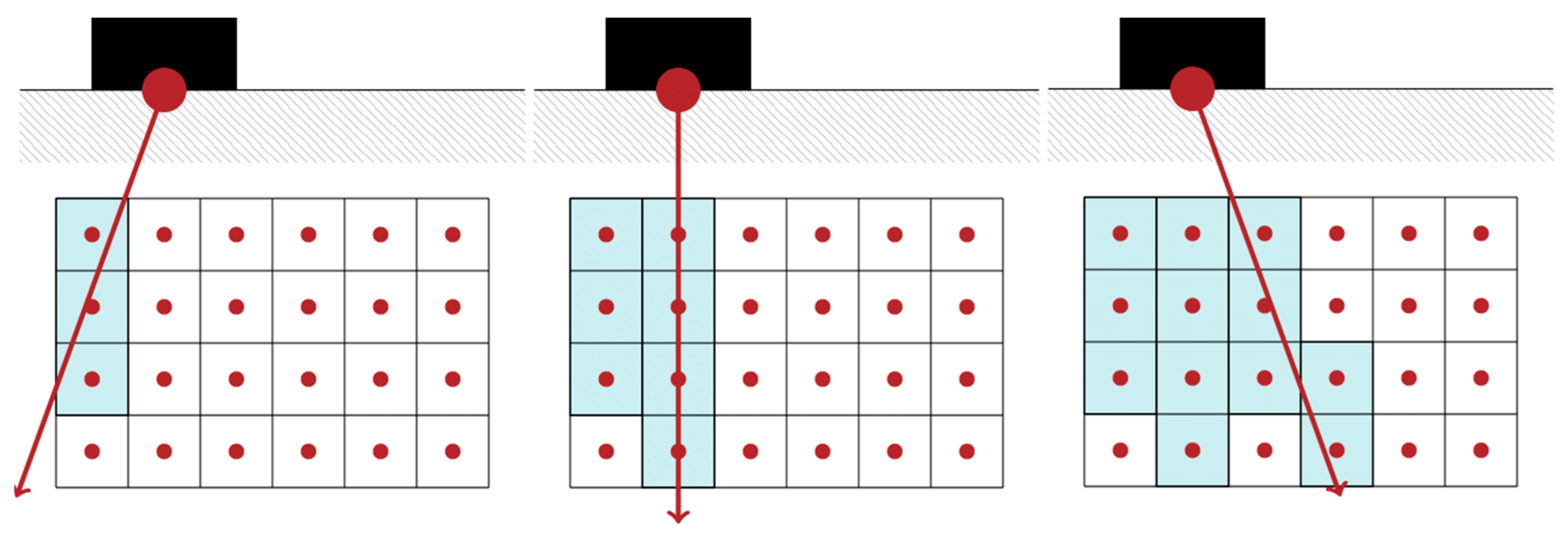
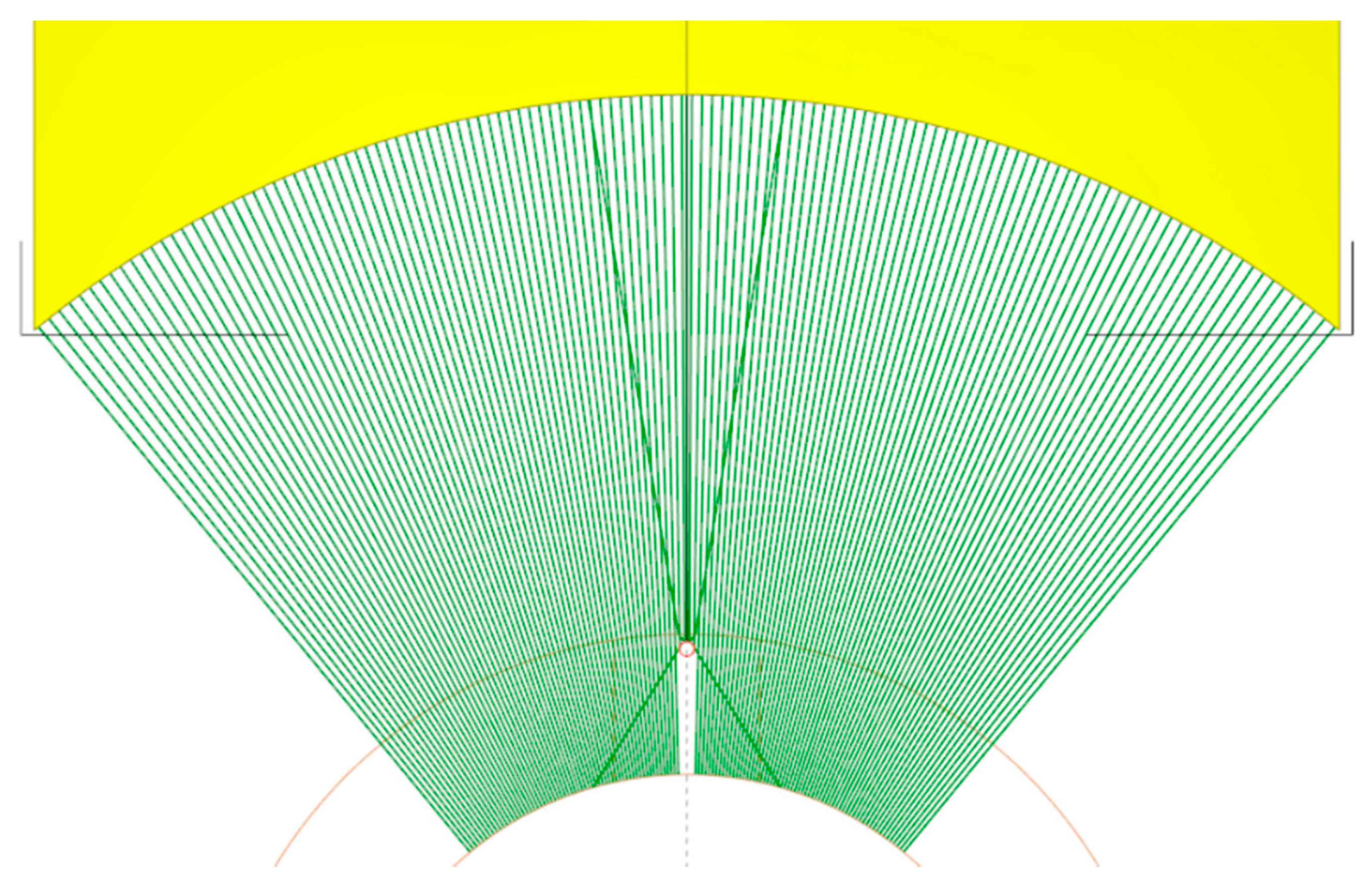
2.4. Raycasting
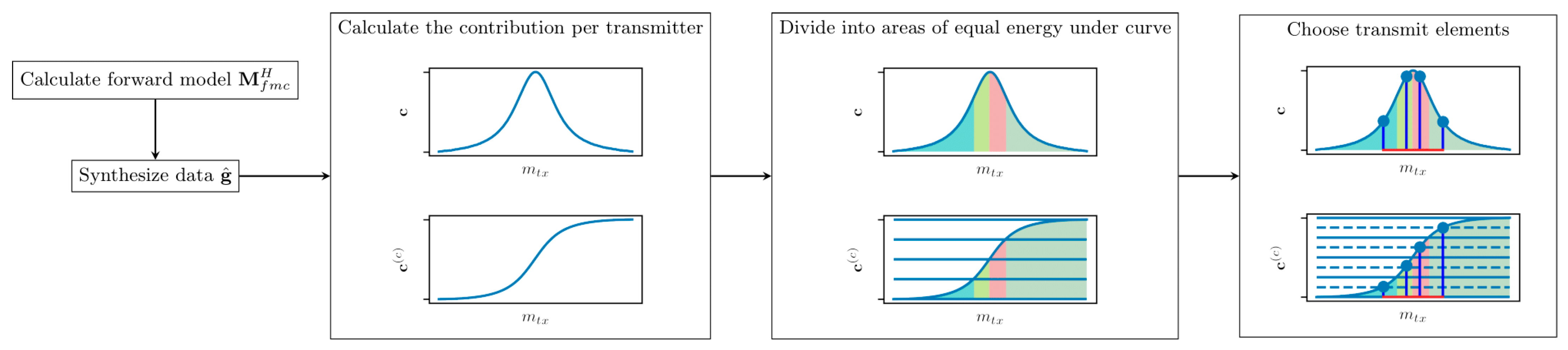
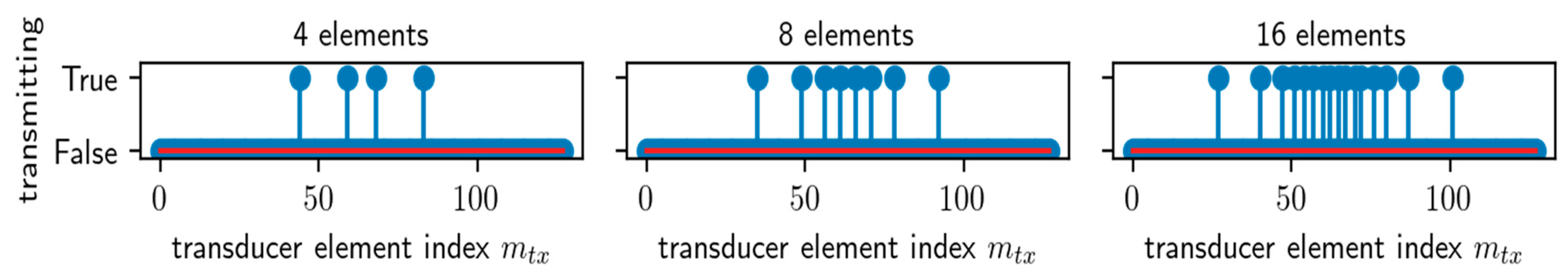
2.5. Transmit Subsampling Strategy
3. Results
3.1. Simulation Scenario
3.2. Transmit Subsampling
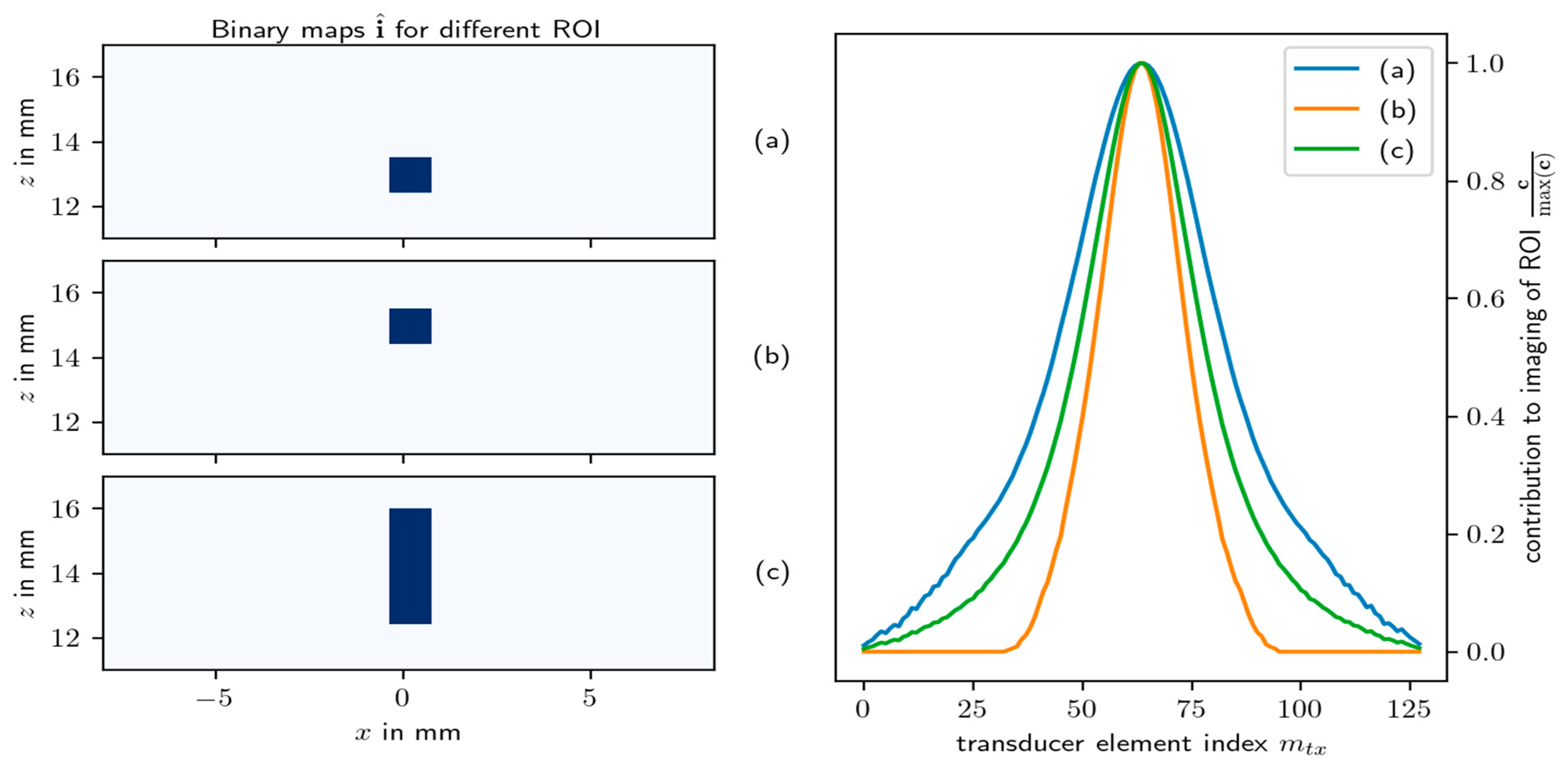
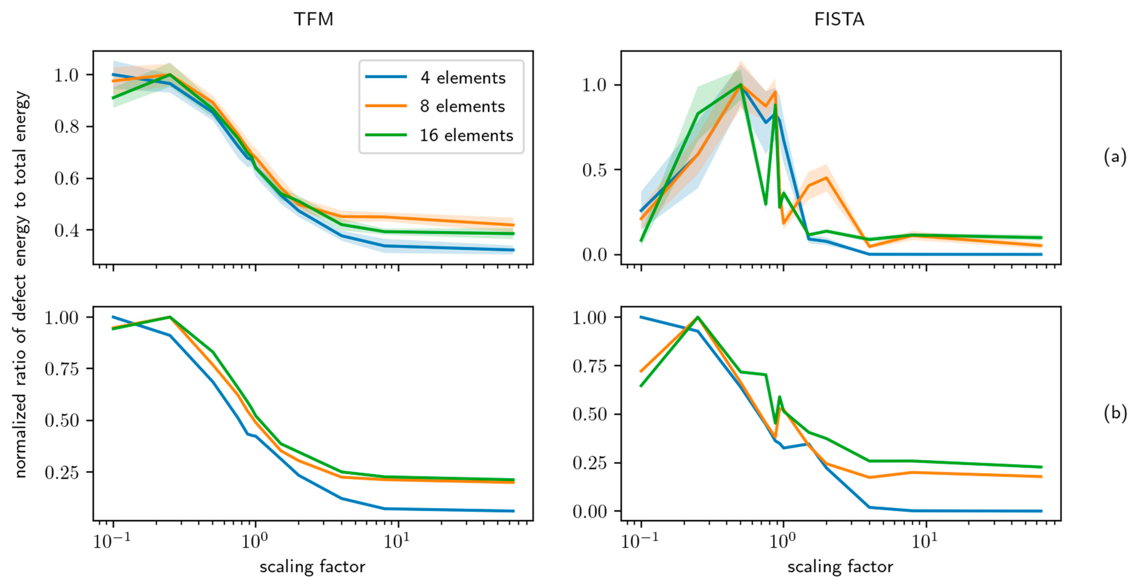
3.2.1. Impact of the Region of Interest Selection
3.2.2. Verification of the Transmit Element Selection Scheme
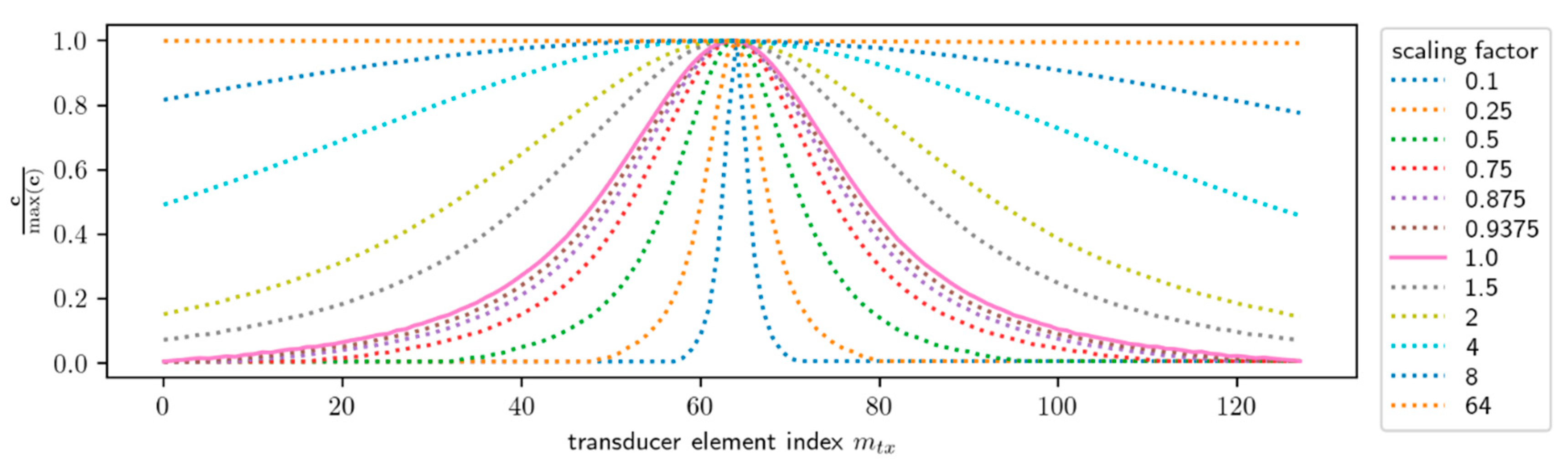
3.2.3. FISTA and the Dictionary Normalization
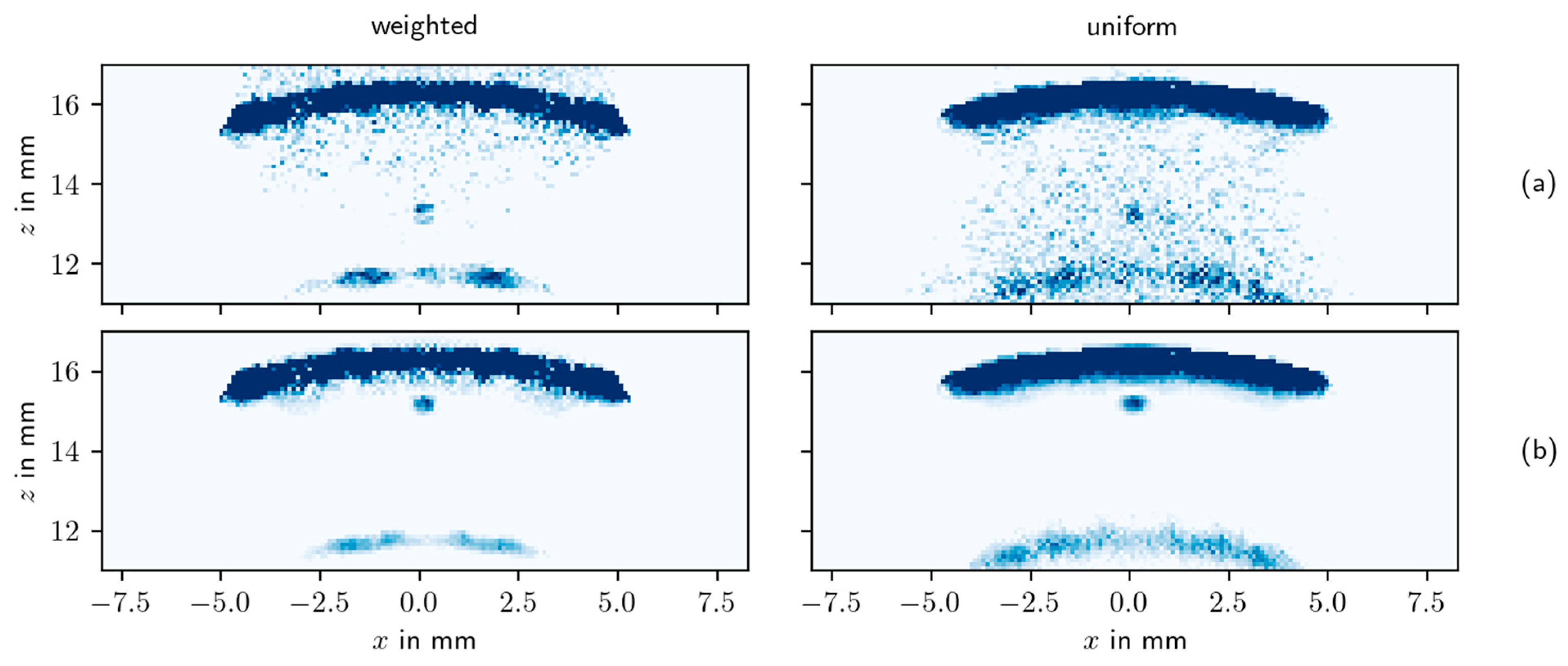
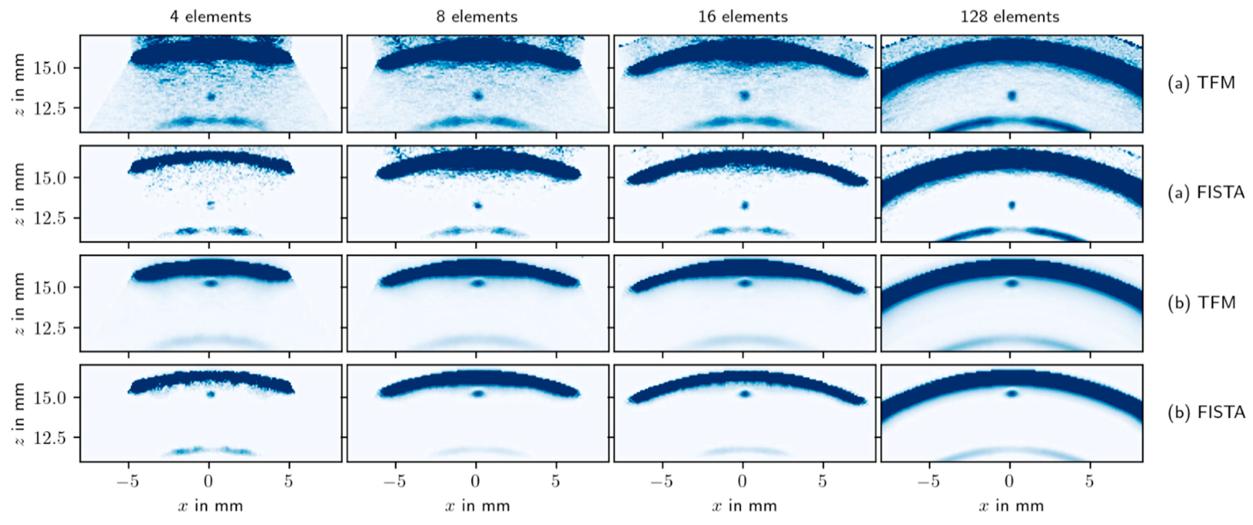
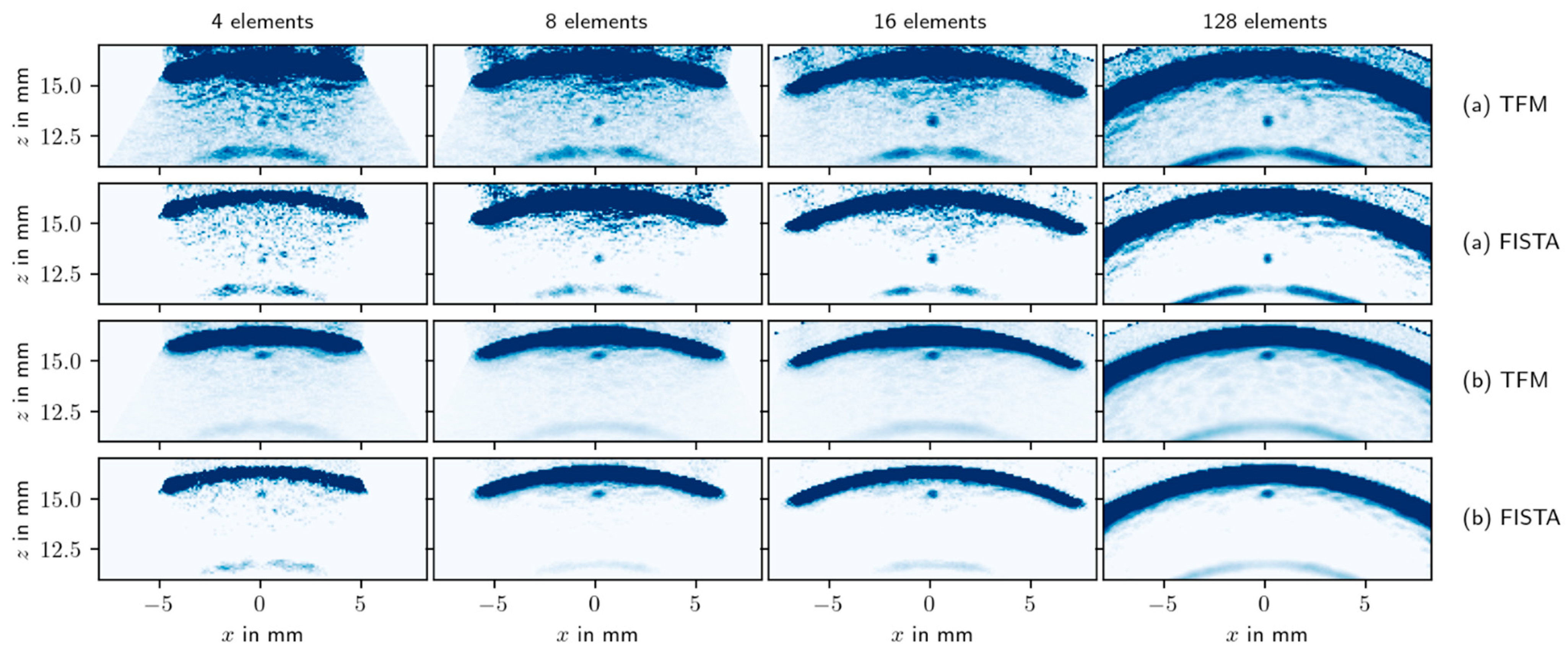
3.2.4. Reconstruction of the Simulated Data
3.2.5. Performance in the Presence of Structural Noise
4. Discussion
Author Contributions
Funding
Institutional Review Board Statement
Informed Consent Statement
Data Availability Statement
Conflicts of Interest
References
- Holmes, C.; Drinkwater, B.W.; Wilcox, P.D. Post-processing of the full matrix of ultrasonic transmit–receive array data for non-destructive evaluation. NDT&E Int. 2005, 38, 701–711. [Google Scholar] [CrossRef]
- Moreau, L.; Drinkwater, B.W.; Wilcox, P.D. Ultrasonic imaging algorithms with limited transmission cycles for rapid nondestructive evaluation. IEEE Trans. Ultrason. Ferroelectr. Freq. Control 2009, 56, 1932–1944. [Google Scholar] [CrossRef] [PubMed]
- Weston, M. Advanced Ultrasonic Digital Imaging and Signal Processing for Applications in the Field of Non-Destructive Testing. Ph.D. Thesis, University of Manchester, Manchester, UK, 2012. [Google Scholar]
- Moreau, L.; Hunter, A.J.; Drinkwater, B.W.; Wilcox, P.D.; Thompson, D.O.; Chimenti, D.E. Efficient data capture and post-processing for real-time imaging using an ultrasonic array. In AIP Conference Proceedings; American Institute of Physics: College Park, MD, USA, 2010; Volume 1211, pp. 839–846. [Google Scholar]
- Hu, H.; Du, J.; Ye, C.; Li, X. Ultrasonic Phased Array Sparse-TFM Imaging Based on Sparse Array Optimization and New Edge-Directed Interpolation. Sensors 2018, 18, 1830. [Google Scholar] [CrossRef] [PubMed] [Green Version]
- Zhang, H.; Liu, Y.; Fan, G.; Zhang, H.; Zhu, W.; Zhu, Q. Sparse-TFM Imaging of Lamb Waves for the Near-Distance Defects in Plate-Like Structures. Metals 2019, 9, 503. [Google Scholar] [CrossRef] [Green Version]
- Zhang, H.; Bai, B.; Zheng, J.; Zhou, Y. Optimal Design of Sparse Array for Ultrasonic Total Focusing Method by Binary Particle Swarm Optimization. IEEE Access 2020, 8, 111945–111953. [Google Scholar] [CrossRef]
- Pérez, E.; Kirchhof, J.; Semper, S.; Krieg, F.; Römer, F. Total focusing method with subsampling in space and frequency domain for ultrasound NDT. In Proceedings of the 2019 IEEE International Ultrasonics Symposium (IUS), Glasgow, UK, 6–9 October 2019; pp. 2103–2106. [Google Scholar]
- Gershon, Y.; Buchris, Y.; Cohen, I. Greedy sparse array design for optimal localization under spatially prioritized source distribution. In Proceedings of the ICASSP 2020 IEEE International Conference on Acoustics, Speech and Signal Processing (ICASSP), Barcelona, Spain, 4–8 May 2020. [Google Scholar]
- Kim, D.; Fessler, J.A. Another Look at the Fast Iterative Shrinkage/Thresholding Algorithm (FISTA). SIAM J. Optim. 2018, 28, 223–250. [Google Scholar] [CrossRef] [PubMed]
- Budyn, N.; Bevan, R.L.T.; Zhang, J.; Croxford, A.J.; Wilcox, P.D. A Model for Multiview Ultrasonic Array Inspection of Small Two-Dimensional Defects. IEEE Trans. Ultrason. Ferroelectr. Freq. Control 2019, 66, 1129–1139. [Google Scholar] [CrossRef] [Green Version]
- Zhang, J.; Drinkwater, B.W.; Wilcox, P.D.; Hunter, A.J. Defect detection using ultrasonic arrays: The multi-mode total focusing method. NDT&E Int. 2010, 43, 123–133. [Google Scholar] [CrossRef]
- Lingvall, F.; Olofsson, T.; Stepinski, T. Synthetic aperture imaging using sources with finite aperture: Deconvolution of the spatial impulse response. J. Acoust. Soc. Am. 2003, 114, 225–234. [Google Scholar] [CrossRef] [PubMed]
- Krieg, F.; Kirchhof, J.; Römer, F.; Pandey, R.; Ihlow, A.; del Galdo, G.; Osman, A. Progressive online 3-D SAFT processing by matrix structure exploitation. In Proceedings of the 2018 IEEE International Ultrasonics Symposium (IUS), Kobe, Japan, 22–25 October 2018. [Google Scholar]
- Wilcox, P.D.; Holmes, C.; Drinkwater, B.W. Advanced Reflector Characterization with Ultrasonic Phased Arrays in NDE Applications. IEEE Trans. Ultrason. Ferroelectr. Freq. Control 2007, 54, 1541–1550. [Google Scholar] [CrossRef] [PubMed]
- Andersen, A.H.; Kak, A.C. Simultaneous Algebraic Reconstruction Technique (SART): A Superior Implementation of the Art Algorithm. Ultrason. Imaging 1984, 6, 81–94. [Google Scholar] [CrossRef] [PubMed]
- Wagner, C.; Semper, S. Fast Linear Transformations in Python. arXiv 2017, arXiv:1710.09578. [Google Scholar]
- Carcreff, E.; Laroche, N.; Braconnier, D.; Duclos, A.; Bourguignon, S. Improvement of the total focusing method using an inverse problem approach. In Proceedings of the IEEE International Ultrasonics Symposium (IUS) 2017, Washington, DC, USA, 6–9 September 2017. [Google Scholar]
- Le Jeune, L.; Robert, S.; Villaverde, E.L.; Prada, C. Plane Wave Imaging for ultrasonic non-destructive testing: Generalization to multimodal imaging. Ultrasonics 2016, 64, 128–138. [Google Scholar] [CrossRef] [PubMed] [Green Version]
- Ogilvy, J. An iterative ray tracing model for ultrasonic nondestructive testing. NDT&E Int. 1992, 25, 3–10. [Google Scholar] [CrossRef]
- Brath, A.J.; Simonetti, F. Phased Array Imaging of Complex-Geometry Composite Components. IEEE Trans. Ultrason. Ferroelectr. Freq. Control. 2017, 64, 1573–1582. [Google Scholar] [CrossRef] [PubMed]
- Bresenham, J.E. Algorithm for computer control of a digital plotter. IBM Syst. J. 1965, 4, 25–30. [Google Scholar] [CrossRef]
- EXTENDE, “CIVA.”. Available online: http://www.extende.com (accessed on 18 March 2021).


| Parameter | Value |
|---|---|
| transducer radius transducer element count transducer element width pitch outer pipe radius inner pipe radius pipe material coupling material | 35 mm 128 0.3 mm 0.05 mm 16.5 mm 11.7 mm Steel Water |
Publisher’s Note: MDPI stays neutral with regard to jurisdictional claims in published maps and institutional affiliations. |
© 2021 by the authors. Licensee MDPI, Basel, Switzerland. This article is an open access article distributed under the terms and conditions of the Creative Commons Attribution (CC BY) license (https://creativecommons.org/licenses/by/4.0/).
Share and Cite
Krieg, F.; Kirchhof, J.; Pérez, E.; Schwender, T.; Römer, F.; Osman, A. Locally Optimal Subsampling Strategies for Full Matrix Capture Measurements in Pipe Inspection. Appl. Sci. 2021, 11, 4291. https://0-doi-org.brum.beds.ac.uk/10.3390/app11094291
Krieg F, Kirchhof J, Pérez E, Schwender T, Römer F, Osman A. Locally Optimal Subsampling Strategies for Full Matrix Capture Measurements in Pipe Inspection. Applied Sciences. 2021; 11(9):4291. https://0-doi-org.brum.beds.ac.uk/10.3390/app11094291
Chicago/Turabian StyleKrieg, Fabian, Jan Kirchhof, Eduardo Pérez, Thomas Schwender, Florian Römer, and Ahmad Osman. 2021. "Locally Optimal Subsampling Strategies for Full Matrix Capture Measurements in Pipe Inspection" Applied Sciences 11, no. 9: 4291. https://0-doi-org.brum.beds.ac.uk/10.3390/app11094291