
Vibration-Based Fingerprint Algorithm for Structural Health Monitoring of Wind Turbine Blades


Institute of Electrical Measurement and Sensor Systems, Graz University of Technology, Inffeldgasse 33/I, 8010 Graz, Austria
*
Author to whom correspondence should be addressed.
Appl. Sci. 2021, 11(9), 4294; https://0-doi-org.brum.beds.ac.uk/10.3390/app11094294
Submission received: 30 March 2021
/
Revised: 29 April 2021
/
Accepted: 5 May 2021
/
Published: 10 May 2021
(This article belongs to the Special Issue Vibration-Based Structural Health Monitoring Ⅱ)
Abstract
:Monitoring the structural health of wind turbine blades is essential to increase energy capture and operational safety of turbines, and therewith enhance competitiveness of wind energy. With the current trends of designing blades ever longer, detailed knowledge of the vibrational characteristics at any point along the blade is desirable. In our approach, we monitor vibrations during operation of the turbine by wirelessly measuring accelerations on the outside of the blades. We propose an algorithm to extract so-called vibration-based fingerprints from those measurements, i.e., dominant vibrations such as eigenfrequencies and narrow-band noise. These fingerprints can then be used for subsequent analysis and visualisation, e.g., for comparing fingerprints across several sensor positions and for identifying vibrations as global or local properties. In this study, data were collected by sensors on two test turbines and fingerprints were successfully extracted for vibrations with both low and high operational variability. An analysis of sensors on the same blade indicates that fingerprints deviate for positions at large radial distance or at different blade sides and, hence, an evaluation with larger datasets of sensors at different positions is promising. In addition, the results show that distributed measurements on the blades are needed to gain a detailed understanding of blade vibrations and thereby reduce loads, increase energy harvesting and improve future blade design. In doing so, our method provides a tool for analysing vibrations with relation to environmental and operational variability in a comprehensive manner.
1. Introduction
Wind energy as a source of renewable energy is one of the essential pillars in the fight against climate change. In 2020, wind energy accounted for 16% of the overall electricity demand in the EU (EU27+UK) [1]. A further increase in capacity is urgently needed to reduce carbon emissions and requires: (i) improving the energy capture per turbine; (ii) reducing the levelised cost of energy; (iii) increasing the number of turbines and parks; and (iv) re-powering of inefficient turbines.
This paper proposes a method for studying the vibrational characteristic of wind turbine blades. Detailed knowledge of the blades’ dynamic response in operation of the turbine is essential: First, blades can optimally be controlled in operation to increase the energy capture. Second, costs can be reduced by reducing loads acting on the blades and thereby prolonging the lifetime of the blades. Blade costs amount to 20% of capital costs and blade damage is responsible for up to 18.2% of downtimes for onshore energy [2,3]. By reducing those costs and downtimes, the competitiveness of wind energy can be increased. Third, monitoring is essential to detect structural changes and damage at an early stage and therewith guarantee safety. Finally, detailed knowledge of the dynamic behaviour of the blade in operation helps engineers in future blade design. With blades being designed ever longer in current trends, this knowledge gets increasingly important since aerodynamic forces as well as costs increase with blade length.
1.1. Related Literature
Blade monitoring refers to both monitoring of vibrations, e.g., fluttering at the blade tip, and monitoring of blade bending, e.g., alternate bending in nonuniform wind profiles. Those two aspects intertwine, i.e., a reduction of blade bending and loads, reduces vibrations and vice versa. This study solely focused on monitoring blade vibrations; however, our proposed sensing principle is also suited for monitoring blade bending as studied in [4]. In general, blade vibrations refer to global properties, e.g., eigenfrequencies, and local properties, e.g., increased vibrations due to fluttering at the blade tip. Both highly depend on environmental conditions such as temperature and wind speed and operational conditions such as rotation speed.
Since measuring the vibrational response is costly and technically challenging, characteristics of blade vibrations have been derived in several simulation studies [5,6,7,8]. Acar and Feeny [5] and Liu et al. [6] demonstrated that eigenfrequencies depend on the stiffness of the blade and vary with operational and environmental parameters. Consequently, eigenfrequencies need to be studied under a large variety of conditions. In addition, Yoo and Shin [7] showed that centrifugal inertia forces increase with both blade length and rotation speed. In addition, Acar and Feeny [5] studied parametric stiffness effects due to centrifugal and gravitational forces and found that the first eigenfrequency of a 100-m blade varied by up to 1.5% with the rotation angle. In all simulation studies, results varied strongly with parameters and respective models. Rafiee et al. [8] summarised beam theories for rotating composite beams such as the Euler–Bernoulli beam theory, the classical beam theory and shear deformation theories with reference to influences such as material nonlinearities, shear stresses and centrifugal stiffening.
Simulations form the basis for further development and testing but can never fully mimic blade properties and environmental conditions. Hence, vibration measurements on wind turbine blades in operation are needed to confirm simulations and investigate vibrations under real-world conditions. Even though few camera-based approaches were developed to monitor vibrations by means of semi-autonomous unmanned aerial vehicles (UAVs) [9] or multiple cameras in a test facility [10], mounting sensors directly on the blades is advantageous in sight-impairing conditions such as fog. In addition, it allows for continuous monitoring during the lifetime of the turbine.
In a small-scale test, Ou et al. [11] conducted a benchmark study and tested accelerometers, force sensors and strain gauges on a turbine blade in a climate chamber. They demonstrated the temperature variability of the frequency characteristic of the blade and proposed further investigation to consider those influences. Moreover, Tcherniak and Mølgaard [12] excited a 34 blade on a test rig by means of an electromechanical actuator inside the blade and collected the vibrational response with an array of accelerometers. Their developed unsupervised learning method was able to detect a 20 damage on the trailing edge based on a damage indicator and a statistical model of the healthy blade. Tcherniak and MØlgaard [13] tested the same algorithm in a follow-up study in operation of a turbine and successfully identified damage. However, the study also demonstrates a major challenge of sensor mounting in real-world applications: Sensors were mounted on the outside of the turbine blade, which resulted in complicated wiring and potentially increased aerodynamic noise. In addition, García and Tcherniak [14] applied active excitation to a 34 blade on a test rig. Damage could successfully be detected; however, sensors had to be mounted in the vicinity of the damage location.
In addition, Bull et al. [15] studied environmental and operational effects with regard to damage detection on an operating Vestas V27 turbine. Accelerometer measurements and weather mast data suggest that temperature and rotation speed highly influence results. In addition, damage detection performed better for actuator excitation than for wind excitation. Last, Al-Khudairi et al. [16] studied the effect of crack propagation in a test facility and determined the frequency response function by using strain gauges and accelerometers. Their experiments demonstrate that damage only leads to minimal changes in eigenfrequencies.
A variety of approaches has been proposed for analysing vibration measurements in related applications, e.g., monitoring of bearings [17,18,19] or bridges [20]. In many approaches, time–frequency-based methods such as empirical mode decomposition [17], wavelets [18] and correlation measures [20] were combined with machine learning and artificial intelligence (AI). For example, Kumar et al. [19] detected bearing defects by using a sparse cost function and convolutional neural networks and therewith addressed the challenges of a small training dataset. However, labelled datasets and precise physical models are unavailable for measurements on wind turbine blades—as occurring for many large-scale structures [21]. Hence, a different approach is needed to analyse those measurements with respect to environmental and operational variability.
1.2. Challenges in Vibration Monitoring
Based on related literature, the following challenges in the monitoring of blade vibrations can be summarised:
- Active excitation of the blade is preferable but mounting of actuators is difficult, especially in retrofit of existing turbines [15].
- Eigenfrequencies can be monitored in a global approach, but a local approach is needed to detect local changes due to damage in the vibrational characteristics [16].
- Reference measurements under damaged conditions are unavailable; hence, analysis methods cannot be based on labelled reference data [21].
1.3. Approach and Objective
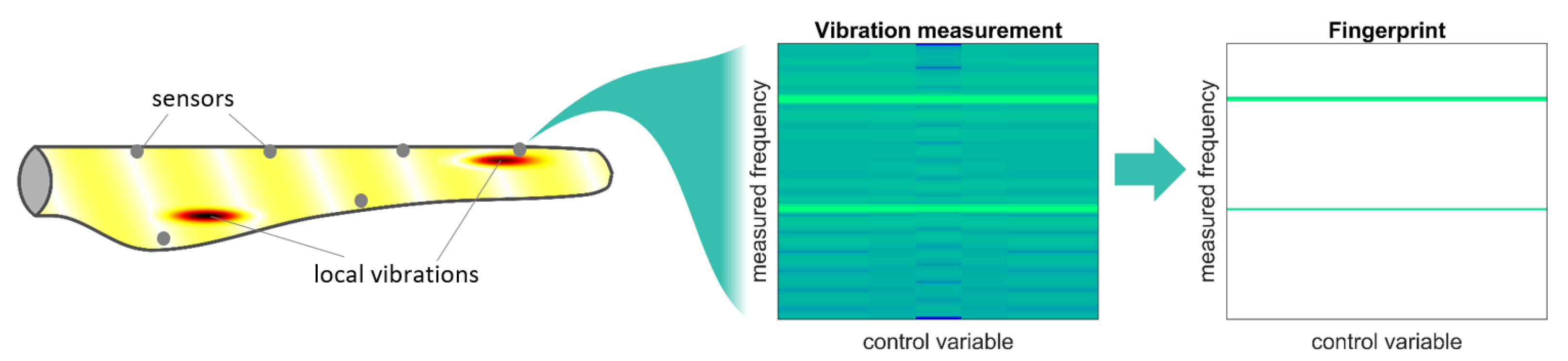
In our approach, we focus on establishing so-called vibration-based fingerprints along different positions of a turbine blade. By mounting accelerometers on the outside of the blade, local vibrations can be monitored at any position. In addition, mounting restrictions due to support structures inside the blades can be avoided. Since actuator mounting is not feasible for existing turbines, we only consider wind excitation. Thereby, our method shall be applicable to existing turbines in retrofit. Vibration measurements at multiple positions along the blade are then used to extract characteristic vibration-based fingerprints, as visualised in Figure 1.
An analysis of spectrograms was proposed by Manhertz et al. [23] for the analysis of laser-vibrometer measurements. Dominant frequencies were extracted for a four-cylinder engine during different operational conditions. Their method was extended [24] by using a moving average predictive method to consider the history of vibrations. Both methods worked well for detecting homogeneous changes in spectra; however, a strategy for identifying inhomogeneous changes is missing, i.e., a dynamic change versus a constant behaviour for adjacent frequencies.
In this study, we propose a method for identifying dominant frequencies in vibration spectra for both homogeneous and inhomogeneous frequency shifts. Extracted dominant frequencies represent both eigenfrequencies and locally increased vibrations, and thereby form characteristic vibration-based fingerprints. An algorithm for efficiently analysing those vibration-based fingerprints is developed and allows for comparing vibrational characteristics at different positions along the blade.
The remainder of this paper is organised as follows. The sensor system and the measurement campaigns are described in Section 2. The proposed algorithm is presented in Section 3, including the detection of vibrations with low and high operational variability in Section 3.3 and Section 3.5, respectively. The results from two test turbines are presented in Section 4. The results are discussed and conclusions are drawn in Section 5 and Section 6, respectively.
2. Experiment
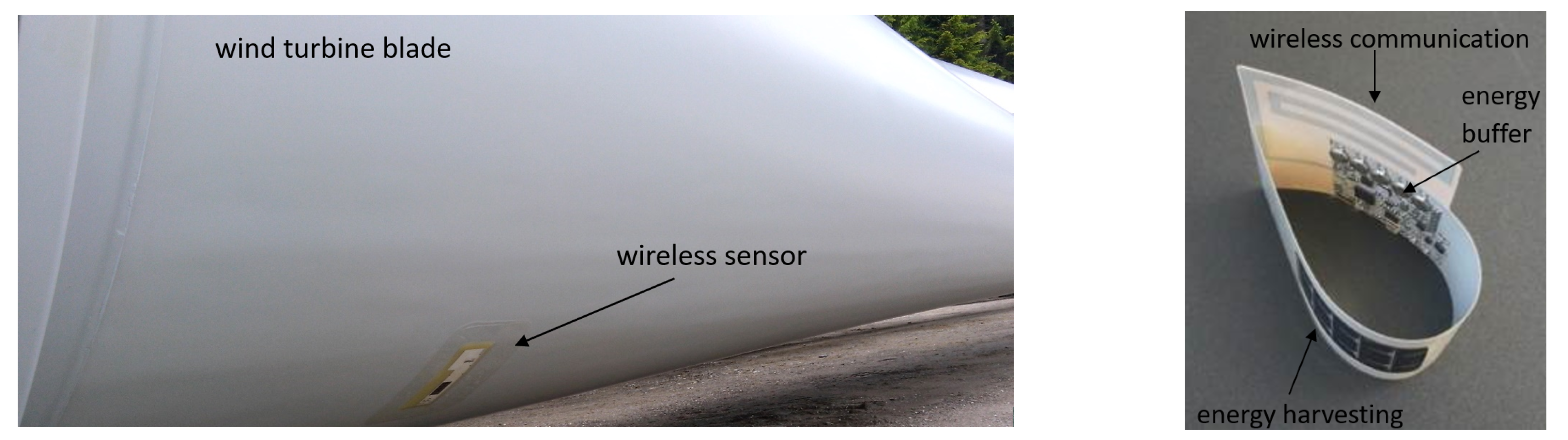
In this section, the sensor system and the test setup are presented. Since our approach aims to measure vibrations at any position along the blade, sensors were mounted on the outside of the blade by using self-adhesive erosion protection tape (see Figure 2). Thereby, placement restrictions on the inside of the blade could be avoided. Vibrations were measured by integrating accelerometers into a robust sensor solution by eologix [25], originally developed for ice detection on the blade. Those sensors are flexible with a thickness less than 2 to minimise additional aerodynamic noise. Any cabling on the outside of the blade is avoided by using solar energy harvesting and a rechargeable energy storage. In addition, wireless communication is used and measured data are transferred to a base station in the tower or nacelle of the turbine.
The wireless prototype sensor used triaxial MEMS accelerometers with a measurement range of g and a sensitivity lower than mg, with 1 g = / corresponding to acceleration due to gravity. Acceleration was measured in measurement campaigns at a sampling rate of 400 (Prototype 1) and 833 (Prototype 2), respectively, for a duration of 10 each with cyclic transmission to the base station. For the proposed analysis method, temporal synchronisation of measurements across sensors was not required but is considered beneficial in future monitoring studies.
Vibration measurements were collected in two test setups: In a 2.5-month test period, Sensors S1 and S2 of Prototype 1 were tested on a 63 rotor blade in operation of the turbine (see Figure 3, left). For this turbine, 1640 and 1100 measurements were available during uniform rotation of the turbine for Sensors S1 and S2, respectively. Measurements during standstill or steering of the turbine, i.e., non-uniform rotational movement, were not taken into account. These measurements were conducted during a large range of environmental and operational conditions and were used to develop our proposed fingerprint method as presented in Section 3.
In addition, an operational 2 MW turbine with a 70 rotor diameter was equipped with Sensors S3–S32 of Prototype 2 in the eastern part of Lower Austria (see Figure 3, right). For those sensors, a maximum of 170 measurements were available from a 2-month test period. Characteristic fingerprints were extracted, and the results are presented in Section 4. For readability, sensor positions are also displayed with results in Section 4.
3. Algorithm
Measured acceleration was analysed by computing vibration-based fingerprints for each sensor position along the rotor blade. In the following, vibrations are classified as Type 1 and Type 2 vibrations:
- Type 1
- Type 2
- Vibrations with large bandwidths and large variation with environmental or operational parameters. For example, vibrations due to fluttering of the blade tip may increase with the rotation frequency.
As a general remark, amplitudes of blade eigenfrequencies are usually small since blade designers try to avoid any excitation of eigenfrequencies along the blade. However, by considering varying environmental conditions and using signal processing methods, those frequencies can also be extracted. Both Type 1 and Type 2 vibrations may correspond to local or global properties of the blade, i.e., may be detected across multiple positions along the blade or only at a selected position. In our analysis, vibration-based fingerprints were created separately for each sensor and, hence, Type 1 and Type 2 vibrations were primarily distinguished by their variability and bandwidth.
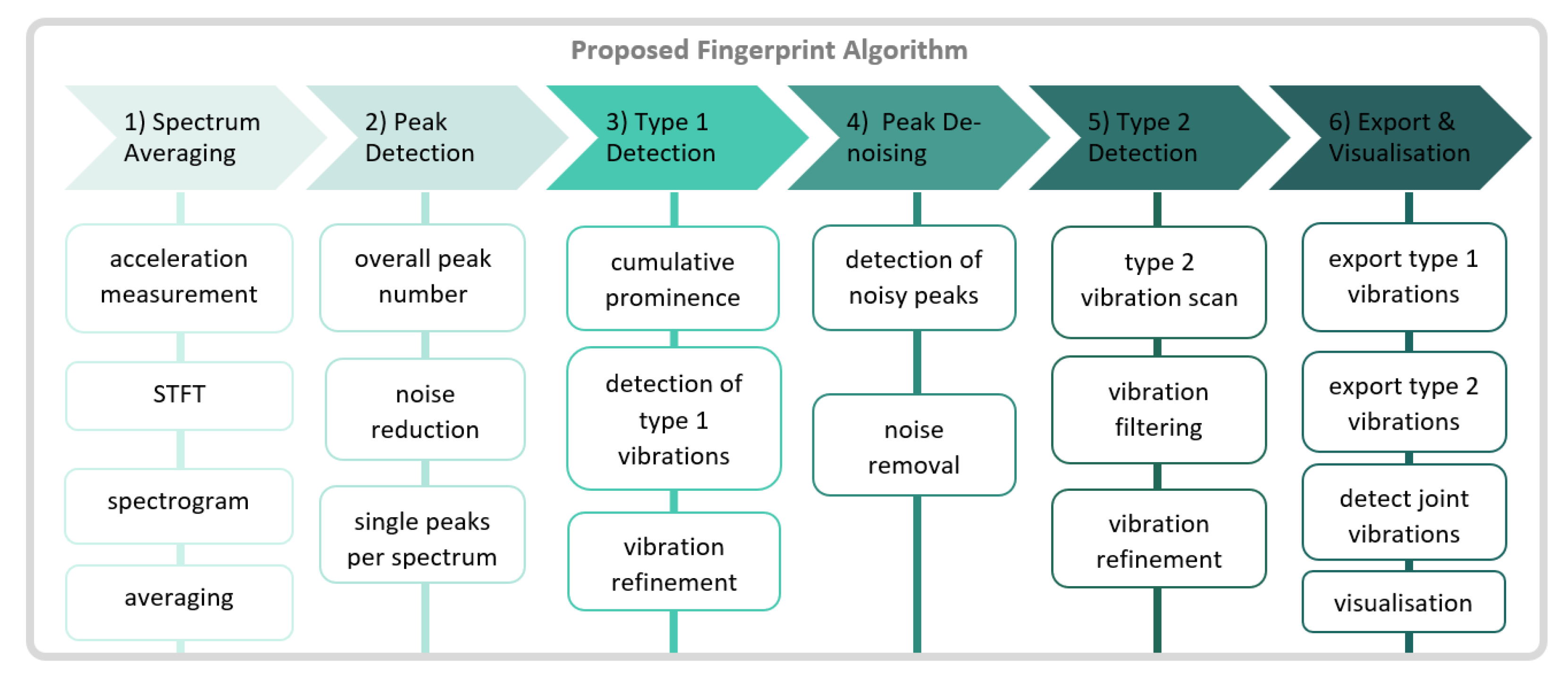
The proposed analysis method consists of six steps, as visualised in Figure 4. First, frequency spectra were computed and resulting spectra were averaged by converting unscheduled measurement campaigns to a reference grid, e.g., the rotation frequency (Spectrum Averaging). Second, dominant frequencies called peaks were identified in computed frequency spectra (Peak Detection). Next, Type 1 vibrations were detected by means of those peaks, i.e., vibrations with small variation with the reference variable (Type 1 Detection). Then, Peak Denoising was conducted and least prominent peaks corresponding to noise were discarded. Last, Type 2 vibrations with large variation with the reference variable were identified by using the remaining set of peaks (Type 2 Detection). Detected Type 1 and Type 2 vibrations were then stored for subsequent analysis. The results were visualised separately or jointly for selected sensors (Export and Visualisation).
The proposed fingerprint algorithm can be applied to vibration measurements in many structural health monitoring applications by adjusting parameters to the properties of measurements. In the subsequent analysis, parameters were empirically selected for acceleration measurements on wind turbine blades. Since vibration measurements collected on Test Turbines 1 and 2 differed with respect to sample size and measurement noise, parameters were adapted separately for each turbine and are specified along with corresponding results in Section 4.
3.1. Spectrum Averaging
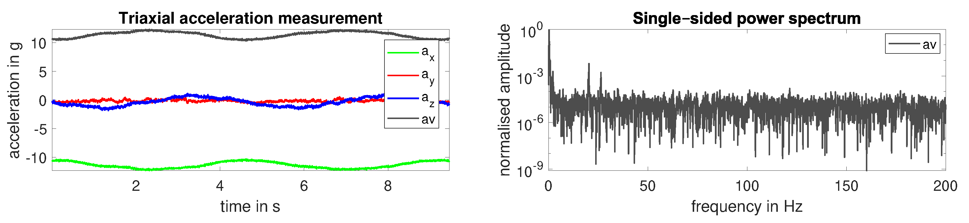
In the following analysis, only measurements during stationary operational conditions were included, i.e., measurements during steering processes or non-stationary rotation speeds were not considered. Since measurements were conducted for a short period of 10 in regular measurement campaigns, the Fourier transform was sufficient to monitor operational and environmental variability and no additional temporal resolution (e.g., by using the Short-time Fourier transform (STFT)) was needed. For each measurement campaign, the Discrete Fourier Transform (DFT) of the signal was computed, and single-sided power spectra were derived as
with the discrete frequency bins corresponding to measured frequencies with and being the sampling rate of the accelerometer. The size of the Fourier transform was selected as to increase precision of frequency detection. The signal was derived from the vector sum of triaxial acceleration measurements with . Thereby, vibration information from three measurement axes could be combined to one fingerprint per sensor location. This procedure also enabled comparability between different sensors in case of a non-ideal alignment of sensor axes to the dimensions of the rotor blade due to mounting tolerances. Most signal energy was contained in the direct current (DC) component of the acceleration signal, which corresponded to centripetal acceleration. Since we focused on analysing vibrations with smaller amplitudes, the DC component was removed. In addition, a Hann window w was applied to account for discontinuities at beginning and end of each measurement campaign. Hence, the signal
was used to compute single-sided frequency spectra, in the following denoted as spectra. Figure 5 displays an exemplary triaxial acceleration measurement and the computed vector sum (left) as well as the corresponding single-sided frequency spectrum (right).
Next, environmental and operational conditions were taken into account to analyse spectrograms. To monitor operational and environmental variability, a separation of variables is needed and sufficient measurements have to be collected for each variable. In our case, measurements were collected during a large range of rotation frequencies, which additionally were expected to have the strongest impact on vibrations. Therefore, the demonstration of the algorithm was based on the rotation frequency as reference variable r. However, any other reference can be applied to the algorithm if a sufficient amount of data is available.
Since measurement campaigns were not scheduled with the reference variable, the number of available measurements was unevenly distributed across the reference. To facilitate visualisation and detection of vibrations, spectra were first sorted by the reference r, i.e., original spectra corresponded to reference measurements with . The resulting set of spectra is denoted as non-linear-scale spectrogram in the following. Reference measurements r were then converted to a fixed grid G of size with a reduction factor R as
For example, a reduction factor of led to an average of 10 measurements per grid point . Spectra corresponding to the linear scale were computed from spectra per grid point i as
with being the averaged spectrum corresponding to reference grid location . Each averaged spectrum was normalised to account for different energy levels. In addition, differences in spectra were enhanced by applying a median filter with length . Resulting spectra are denoted as linear-scale spectra, short spectra in the following. In addition, the resulting set of spectra is denoted as linear-scale spectrogram.
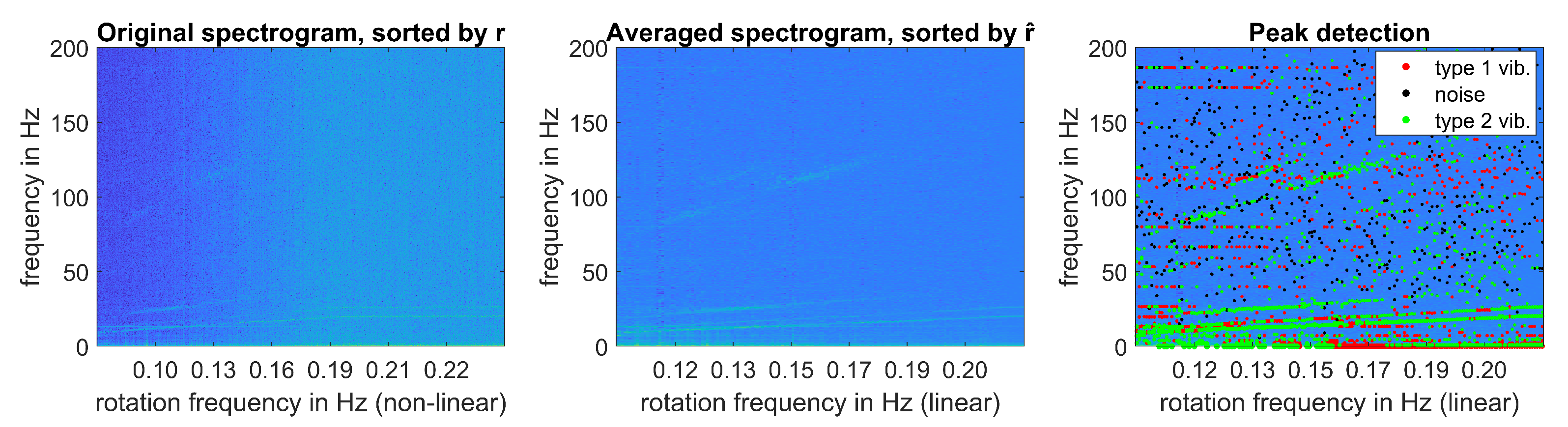
Figure 6 displays original spectra sorted by the rotation frequency (reference r) on a non-linear scale (left) and averaged spectra on the linear scale (middle). Averaging of spectra notably reveals vibrations, which are otherwise hidden by noise. In addition, vibrations appear more significant and noise is reduced. The following processing steps were used to automatically extract those vibrations in the spectrogram, which are easily detected by the eye. The analysis is split into the detection of Type 1 and Type 2 vibrations (see Section 3.3 and Section 3.5, respectively).
3.2. Peak Detection
The fingerprint algorithm is based on the detection of prominent frequencies called peaks in the linear-scale spectrogram. In doing so, the prominence of peaks, i.e., the height of a peak with reference to the closest local minimum, is essential to identify prominent frequencies with relation to respective frequency bands and independently of overall peak amplitudes. As a preparatory step, peaks were identified separately in each linear-scale frequency spectrum.
First, an estimate of the overall number of peaks was derived by using the averaged linear-scale spectrogram
on a logarithmic scale, i.e., . The overall number of peaks was determined in the signal by detecting peaks with a minimum prominence of . This means that the height of peaks had to exceed the corresponding local minima by at least . In addition, only peaks with a minimum distance of 10 frequency bins k to the next peak were considered. Thereby, the high variability of the signal was taken into account and only one peak per relevant component was detected.
The overall number was then used to select the number of single peaks, which should be identified per linear-scale spectrum. The best trade-off between minimum noise and a maximum number of prominent peaks had to be found empirically for each measurement setup. A reduction factor of was introduced and the most prominent peaks were detected for each linear-scale spectrum. In the following analysis, peaks are described by their prominence , width and location , with corresponding to the reference grid and peak numbers n corresponding to discrete frequency bins k with . Figure 6 (right) displays detected peak locations with colours corresponding to their properties (i.e. related to Type 1 and Type 2 vibrations or noise) as derived subsequently in Section 3.3, Section 3.4 and Section 3.5.
3.3. Detection of Type 1 Vibrations
As a first step, extracted peaks were analysed with regard to Type 1 vibrations, i.e., those peaks were identified, for which peak locations exhibited a low variation with the rotation frequency.
3.3.1. Identification of Type 1 Vibrations
Those discrete frequency bins k were identified for which peaks were most frequently detected. The prominence of peaks was analysed with respect to discrete frequencies as
in other words, all peaks were projected on the frequency axis and corresponding prominences were summarised. To enable automatic detection of those locations, the projected prominence was smoothed by accumulating within frequency bands . The width factor was selected empirically for each test turbine.
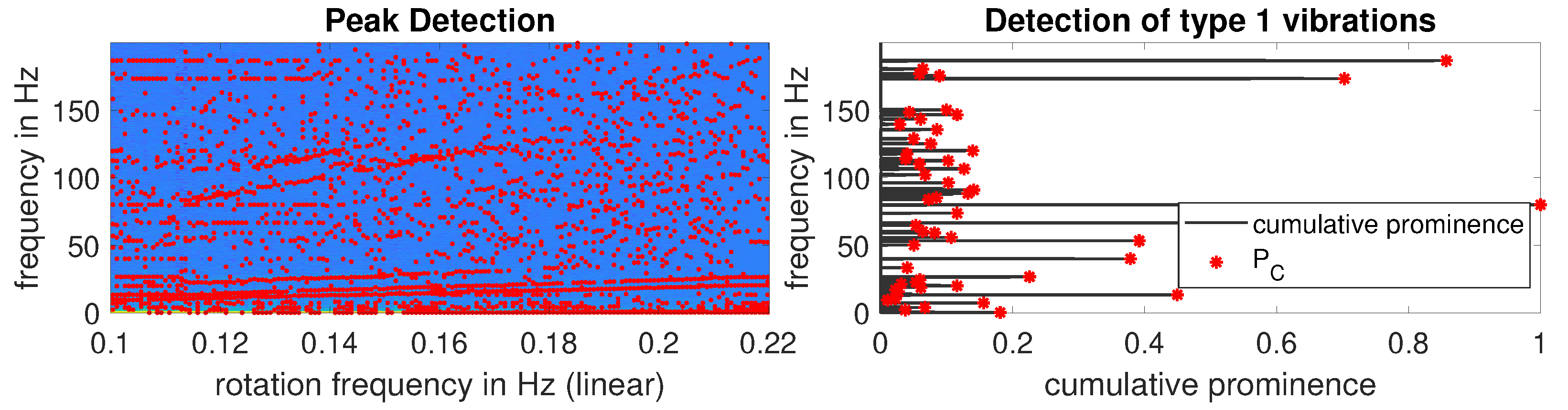
The resulting cumulative prominence was then used to detect most prominent peaks with a minimum peak prominence of . Here, the minimum peak prominence was empirically selected and resulted in the detection of peaks in total. Those peaks corresponded to frequency bins k in the linear-scale spectrogram, which: (i) occurred across a significant range of the operational range (here, rotation frequency; general. reference variable ); and (ii) only slightly varied with . Hence, they fulfilled the properties of Type 1 vibrations as defined in this section. Those peak locations and peak widths determined the set of Type 1 vibrations at frequency bins and with width for , respectively, in the following analysis. Figure 7 displays the locations of all peaks, cumulative prominence and most prominent peaks corresponding to identified Type 1 vibrations .
3.3.2. Refinement of Type 1 Vibrations
For each identified Type 1 vibration , all corresponding peaks in the linear-scale spectrogram were identified. If fewer than five peaks were identified, the vibration was considered invalid and removed from the result set. For each remaining Type 1 vibration, the set of all peaks was created with elements for and . Those peaks were used to derive the dependency on the reference variable by fitting the first-degree polynomial
to identified peak locations by using robust linear least squares fitting. Here, and corresponded to the fitting parameters for vibration and estimated functions represent the variation of discrete frequencies with the reference.
Resulting functions were stored for further analysis. The majority of peaks corresponding to each Type 1 vibrations (67%) were removed from the set of all identified peaks . However, the most prominent 33% of peaks corresponding to each Type 1 vibration j were kept in the dataset to account for potential overlaps of Type 1 and Type 2 vibrations. All peaks related to Type 1 vibrations are displayed in Figure 6 (right) in red colour. In addition, peak locations corresponding to Type 1 vibrations are displayed in Figure 7 (right).
3.4. Peak Denoising
In the next step, peaks with low prominence were removed to increase the signal-to-noise ratio. Those peaks may either result from eigenfrequencies or sensor noise. Since blade design tries to prevent the excitation of eigenfrequencies, they can only be detected as peaks with low amplitudes and low prominence. Hence, peaks with low prominence were needed for Type 1 Detection to increase detection accuracy. In contrast, peaks with low prominence reduced the signal-to-noise ratio in the detection of Type 2 vibrations as done in in the next step (Type 2 Detection) and therefore corresponded to noise. Consequently, peaks with low prominence were removed as an intermediate step.
A factor was introduced and those peaks with lowest prominence per linear-scale spectrum were assigned to a set of noisy peaks . The set of noisy peaks was then excluded from subsequent analyses. Thereby, the factor provided a trade-off between sensitivity to Type 2 vibrations and robustness of the subsequent algorithm and was selected separately for each test turbine. The set of noisy peaks is displayed in Figure 6 (right) with dots in black colour. In the following step, the set of peaks was scanned for peaks corresponding to Type 2 vibrations ().
3.5. Detection of Type 2 Vibrations
From the remaining set of peaks , those peaks corresponding to Type 2 vibrations were identified, i.e., those vibrations related to a large variation with the reference variable. The subsequent algorithm can be split in three parts, which are (i) scanning of Type 2 vibrations, (ii) filtering of the scan result to detect the most prominent vibrations and (iii) refinement of detected Type 2 vibrations.
3.5.1. Scanning of Type 2 Vibrations
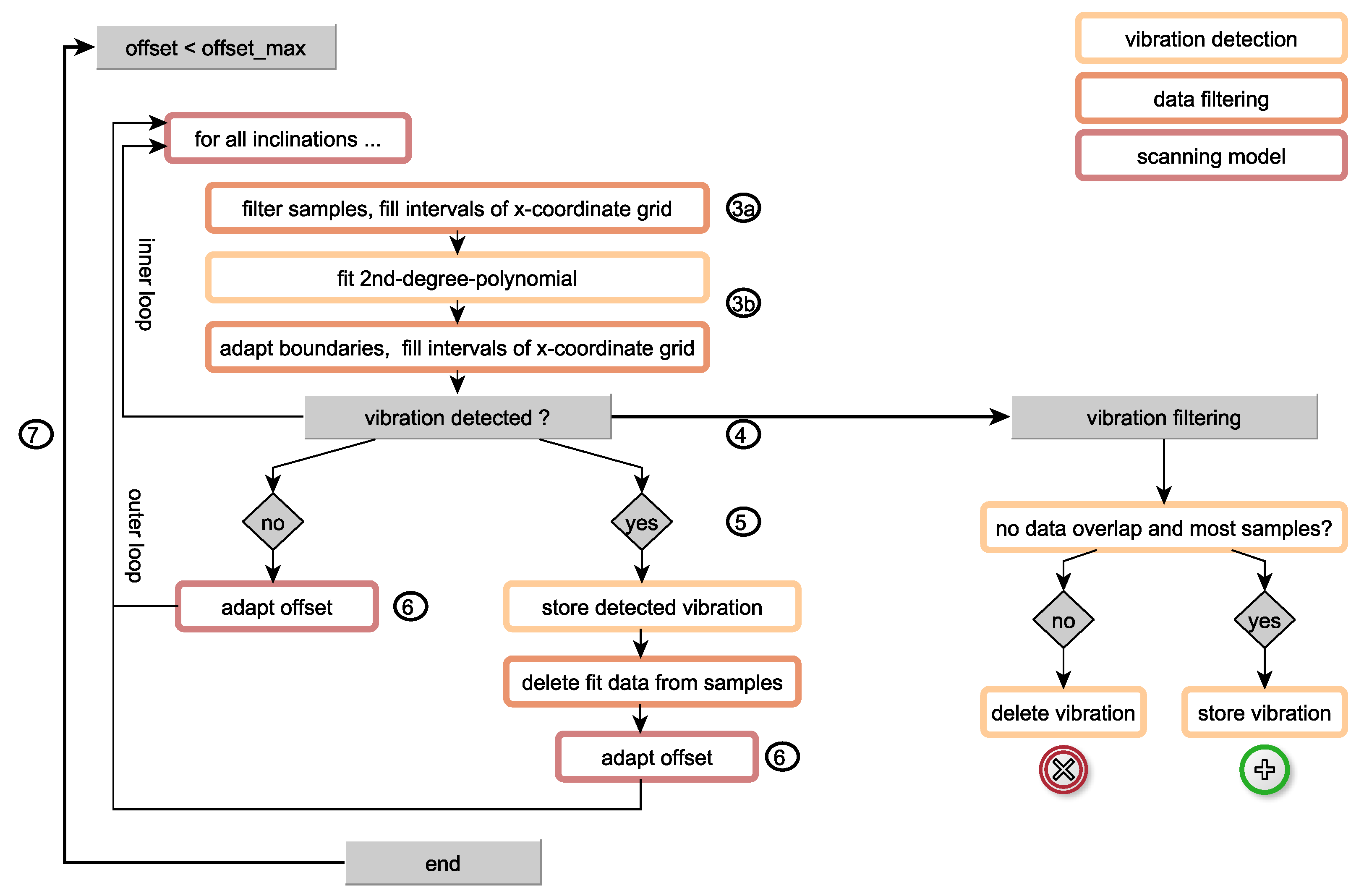
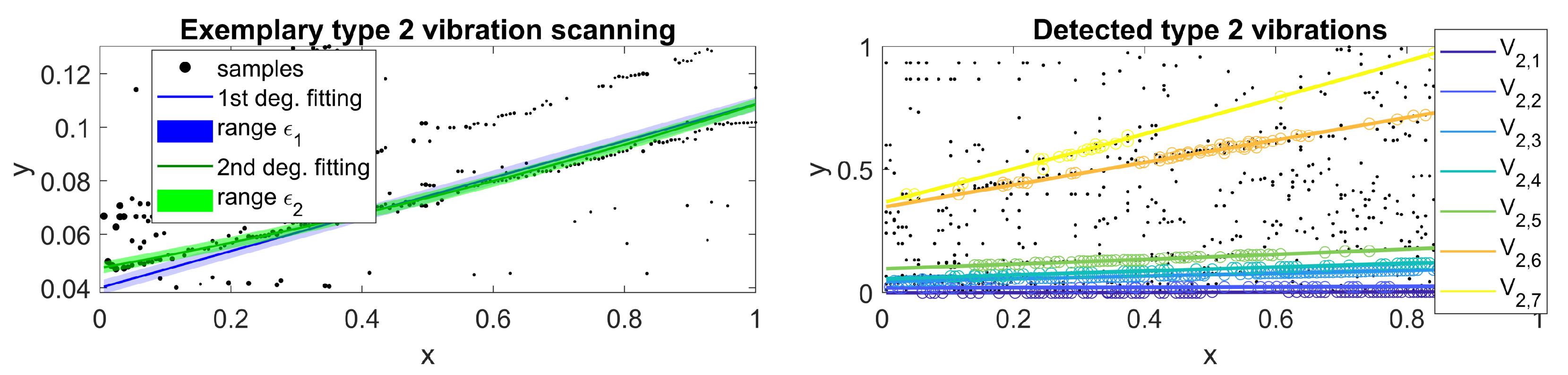
First, peaks were scanned for those peaks corresponding to Type 2 vibrations. The algorithm is displayed in Figure 8, left:
- The location of remaining peaks as resulting from Section 3.4 was normalised, i.e., both the range of and were normalised to [0,1]. Normalised peaks are denoted as samples during the scanning part of the algorithm, and each peak was converted to a sample with coordinates and and .
- Those samples were scanned by using first- and second-degree polynomials (see Figure 8). For each outer loop iteration, an offset was fixed. For each inner loop iteration, inclinations were varied in steps of up until a maximum inclination of . Parameters , , and were selected empirically based on the location of remaining peaks , as displayed in Figure 6 (right) (green colour).
- For given and , the following steps were conducted:
- (a)
- The x coordinate [0,1] was divided into discrete intervals . The model was created for each iteration, and a boundary with was introduced. This boundary was increased up until at least one of the following conditions was fulfilled:
- Strict: For at least of intervals, at least one sample had to be found per interval which fulfilled .
- Interval: For vibrations only occurring for specific values of the reference variable, an additional restricted range was introduced. In this range, Condition (i) had to be fulfilled for at least samples.
- (b)
- The model was refined by fitting a second-degree polynomial to all those samples , for which in the previous step. Linear least squares fitting was used and the prominence of peaks related to samples were used as fitting weights. Again, the two conditions for defining the range were applied as defined in Step 3(a) for a range . An example for both first- and second-degree polynomial fits and ranges is shown in Figure 9 (left).
- Those models with a sum of squared errors (SSE) lower than a maximum error were selected as Type 2 vibrations and stored for further processing. In our analysis, was selected empirically for each test turbine depending on respective data quality.
- For each detected vibration, fit parameters , , and were stored. In addition, all samples for which were saved for subsequent analyses. To improve robustness of scanning from bottom () to top (), samples for which ) were removed from the overall set of samples for the next iteration.
- The offset was adapted and increased by for the next iteration if either a vibration was successfully detected or all inclinations were tested without success.
- Steps 3–6 were repeated up until the maximum offset was reached.
Here, only inclinations were tested since vibrations always increased with the reference variable (rotation frequency) in our datasets. The algorithm can easily be extended to also consider negative correlations by testing .
3.5.2. Filtering of Scan Results
Second, scan results were filtered for the most prominent vibrations (see Figure 8, right). Since scanning was conducted from bottom to top, only the lower part of corresponding samples was deleted in Step 3(b) to increase robustness of fitting. Consequently, samples could be assigned to a different vibration in the next iterations.
Hence, for each vibration , it was tested if there was a vibration for which
- At least 10% of samples were assigned to both vibrations and .
- A larger number of samples was assigned to vibration .
If these conditions were fulfilled, vibration was deleted from the result set. The remaining vibrations with constituted the set of successfully scanned Type 2 vibrations (e.g., see Figure 9, right). Detected peaks corresponding to those vibrations are denoted as . Overall, the number of peaks as detected in Section 3.2 can be written as with being those peaks, for which no significant vibrations could be extracted in Section 3.5. The joint set is displayed in Figure 6 (right) in green colour.
3.5.3. Refinement of Type 2 Vibrations
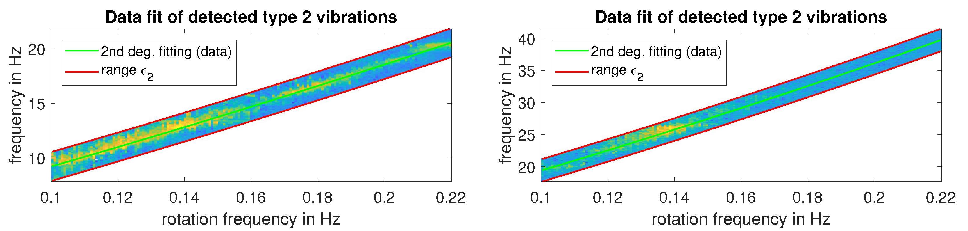
While detected peaks and samples were considered during vibration scanning, Type 2 vibrations were then refined by considering linear-scale spectrograms. For this, normalised samples were converted back to peak locations . In addition, boundaries were adapted from the normalised range to and models were adapted to . Then, refinement was conducted for each Type 2 vibration :
- A grid with elements was created with and .
- Each model was refined by using spectra information as fitting weights for data points ,
- Robust fitting was used as with parameters , and .
An example of two Type 2 vibrations for the exemplary sensor is displayed in Figure 10.
3.6. Export and Visualisation
Finally, detected Type 1 and Type 2 vibrations were combined to a characteristic vibration-based fingerprint. Each fingerprint consisted of the following properties:
- Type 1 vibrations with including detected peaks , first-degree fitting models and corresponding data ranges .
- Type 2 vibrations with including detected peaks , second-degree fitting models and corresponding data ranges .
Those fingerprints were stored for the subsequent analysis of results. Algorithm results were visualised by displaying averaged spectrograms, fingerprints and sensor positions (see, for example, Figure 11). Thereby, characteristic vibrations of Type 1 () and Type 2 () were visualised by displaying fitting models as solid lines. The prominence of assigned peaks and the range of vibrations were considered by: (i) normalising the prominence of assigned peaks to [0,1] (relative width); and (ii) scaling the range of each vibration (absolute width) with the normalised prominence. In doing so, the maximum width of each visualised vibration corresponds to the deviation of peak locations of the respective vibration. In addition, the variation of the width over the reference variable corresponds to the prominence of assigned peaks. Thereby, the following properties can be visualised:
- A large absolute width of vibrations indicates that the vibration is difficult to localise, e.g., due to an additional dependency on further environmental or operational parameters.
- A small relative width of vibrations indicates that the vibration is difficult to detect, e.g., either not excited or hidden in noise for the related reference .
- A large relative width of vibrations indicates that the vibration can clearly be identified in the linear-scale spectrogram.
In addition, fingerprints were compared for several sensors. Two vibrations and were detected as joint or overlapping, i.e., being caused by the same physical behaviour of the blade with high probability if any of the following conditions applied:
- (i)
- At least 30% of assigned peaks overlapped: A number of joint peaks was found with being the number of peaks and being the number of peaks .
- (ii)
- The difference at any point along the reference grid was smaller than 1.5%, i.e., .
In the case of joint vibrations being detected, vibrations and were averaged to increase clarity of visualisation. Averaged vibrations are displayed by alternating coloured dots and error bars represent the width of single vibrations. An example for the visualisation of joint vibrations can be seen in Figure 12.
4. Results
The fingerprint algorithm was tested by using measurements from several sensors, which were mounted on two test turbines as discussed in Section 2. The results are presented using the methods described in Section 3.6 for visualising fingerprints both separately per sensor and jointly for several sensors. The following section is split into results regarding Turbine 1 (Section 4.1), results regarding Turbine 2 (Section 4.2) and a joint evaluation for sensors on both turbines (Section 4.3). Parameters of the fingerprint algorithm were adjusted separately for sensors of both test turbines to account for: (i) varying vibration characteristics of the turbines; and (ii) varying size and data quality of sensor measurements (see Table 1). However, parameters were kept constant for sensors of the same turbine to enable comparability of results. Selected parameters are discussed subsequently and the reader is referred to Section 3 for a detailed description of the full set of algorithm parameters.
4.1. Test Turbine 1
For the first test turbine, the two Sensors and were mounted at the blade tip at 88% and 98% of the blade length, respectively. The fingerprint algorithm was applied to the dataset of each sensor separately and parameters were adjusted as displayed in Table 1. Since the dataset was large with 1640 and 1100 measurements for Sensors and , respectively, the reference grid could be set to a high resolution with 7 × 10. This led to a large number of averaged spectra and, thus, a low noise level, which allowed localising Type 1 vibrations with a width of = 1 × 10. In addition, parameters were set separately for the lower part () and the upper part () of the data range during the detection of Type 2 vibrations. Thereby, different properties of measurements such as well-localised and adjacent vibrations in the lower part of spectrograms and vibrations with large bandwidth in the upper part of spectrograms were considered.
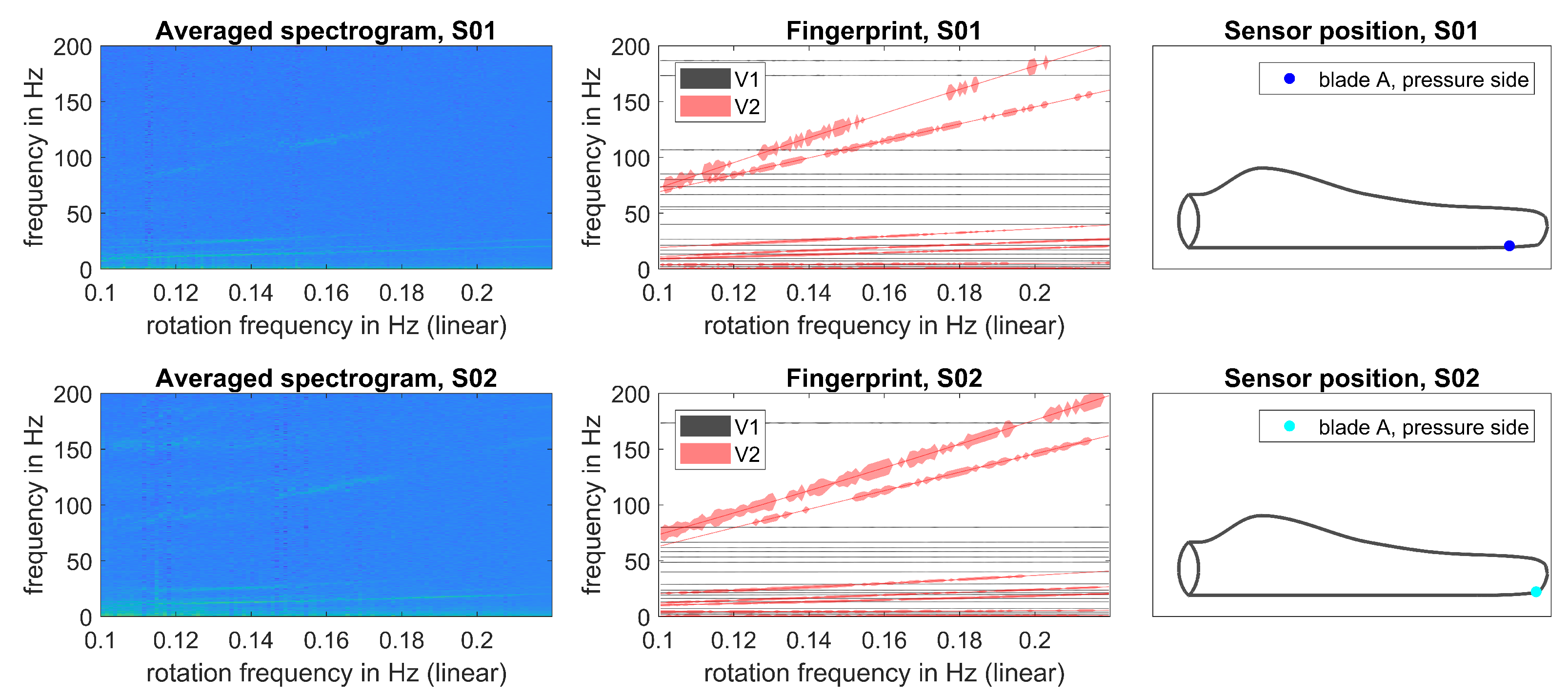
Algorithm results for Sensors and are presented in Figure 11. In averaged spectrograms, several distinct Type 2 vibrations are visible below 25 and two Type 2 vibrations with higher bandwidth appear in the higher frequency range above 75 . In addition, higher noise levels are visible for Sensor , which was mounted further towards the tip of the blade. Extracted vibration-based fingerprints show that Type 2 vibrations were correctly identified and extracted from averaged spectrograms. In those vibrations, a larger bandwidth of vibrations reflects higher noise levels for Sensor . Furthermore, several Type 1 vibrations width small bandwidth were identified for both sensors corresponding to either eigenfrequencies of the blade or increased narrow-band noise. These vibrations are only visible in averaged spectrograms by a detailed close-up view; hence, the fingerprint algorithm can be used for automatic extraction.
A comparison of both fingerprints is displayed in Figure 12. All Type 2 vibrations could successfully be measured and detected by both sensors. For Sensor , the highest vibration (first from top) was detected for a larger range of rotation frequencies than for Sensor . This is represented by coloured error bars at those rotation frequencies, for which peaks were assigned to the respective vibration. The majority of Type 1 vibrations were detected by both sensors. Those vibrations exclusively being detected by Sensor indicate eigenfrequencies with small amplitudes, which are hidden in noise for Sensor . In contrast, Type 1 vibrations exclusively being detected for Sensor indicates a detection of sensor noise in distinct narrow-band frequencies.
To sum this up, fingerprints of both sensors overlap for the majority of vibrations since the radial difference between both sensors is small. However, higher vibrations at the blade tip, e.g., due to fluttering, are reflected in the fingerprint of Sensor by the location of detected Type 1 vibrations and the bandwidth of Type 2 vibrations.
4.2. Test Turbine 2
For the second test turbine, Sensors – were mounted on all three blades of the turbine. For comparability, selected sensors were deployed at the same positions on all blades. Additional sensors were deployed at varying positions on the first blade (Blade A) for a closer inspection of different positions along the blade. It needs to be noted that the set of available measurements was much smaller for this turbine (9–15% with reference to sensors on Test Turbine 1) and both size of datasets and data quality (e.g., increased noise due to transmission errors) varied across sensors. Therefore, only selected sensors were considered in the subsequent evaluation.
Due to smaller datasets, averaging of spectrograms had to be conducted with fewer measurement campaigns per grid point. Hence, averaged spectrograms of Turbine 2 included higher noise levels. Parameters were adapted as displayed in Table 1:
- adaption of grid resolution with 5 × 10;
- reduction of peaks to reduce noise for Type 1 detection ();
- less noise reduction to find Type 2 vibrations hidden in noise ( = 0.25);
- increased sensitivity to Type 2 vibrations hidden in noise (); and
- increased range limits ( 3 × 10).
In addition, parameters were adjusted separately for three different parts of the data range, i.e., a lower part (), a middle part () and an upper part (). The interval condition was used for the middle and upper part to increase sensitivity to those vibrations, which did not occur for the full operational range of the turbine.
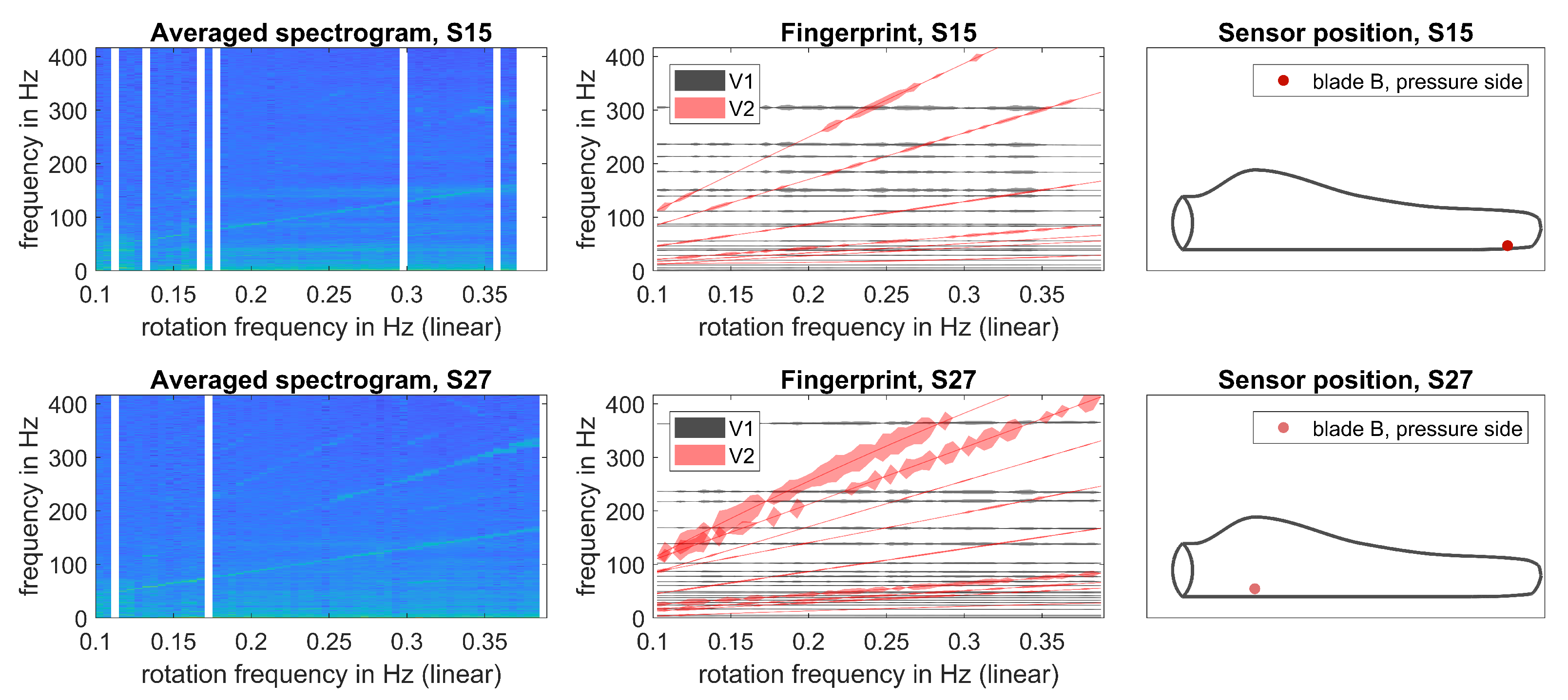
Figure 13 displays exemplary fingerprints for Sensors and mounted on tip and root of a rotor blade on Test Turbine 2. The effects of the smaller datasets are reflected in: (i) white gaps in averaged spectrograms representing missing measurements for respective grid points; and (ii) higher measurement noise, especially below 100 . The fingerprint algorithm identified several Type 2 vibrations, which correspond to those vibrations clearly visible in averaged spectrograms. By using the interval condition for detection, vibrations only occurring for parts of the operational range could be identified, e.g., see Sensor with Vibrations 2 and 4 from the top.
Due to increased measurement noise, only Type 1 vibrations with large bandwidths were detected. For frequencies below 75 , those frequencies mostly overlapped with Type 2 vibrations and, hence, decreased accuracy of Type 2 detection. Therefore, the following analysis is focused on analysing Type 2 vibrations above 75 . Fingerprints for Sensors and only partly overlap for Type 2 vibrations and, hence, the properties of fingerprints of different sensors are evaluated in the following with respect to sensor positions. Due to the implications of data quality as discussed, only indications can be given in the following, and final conclusions on the vibrational characteristics of the blades, optimal sensor deployment, etc. need to be confirmed by larger datasets.
4.2.1. Comparison of Radial Positions
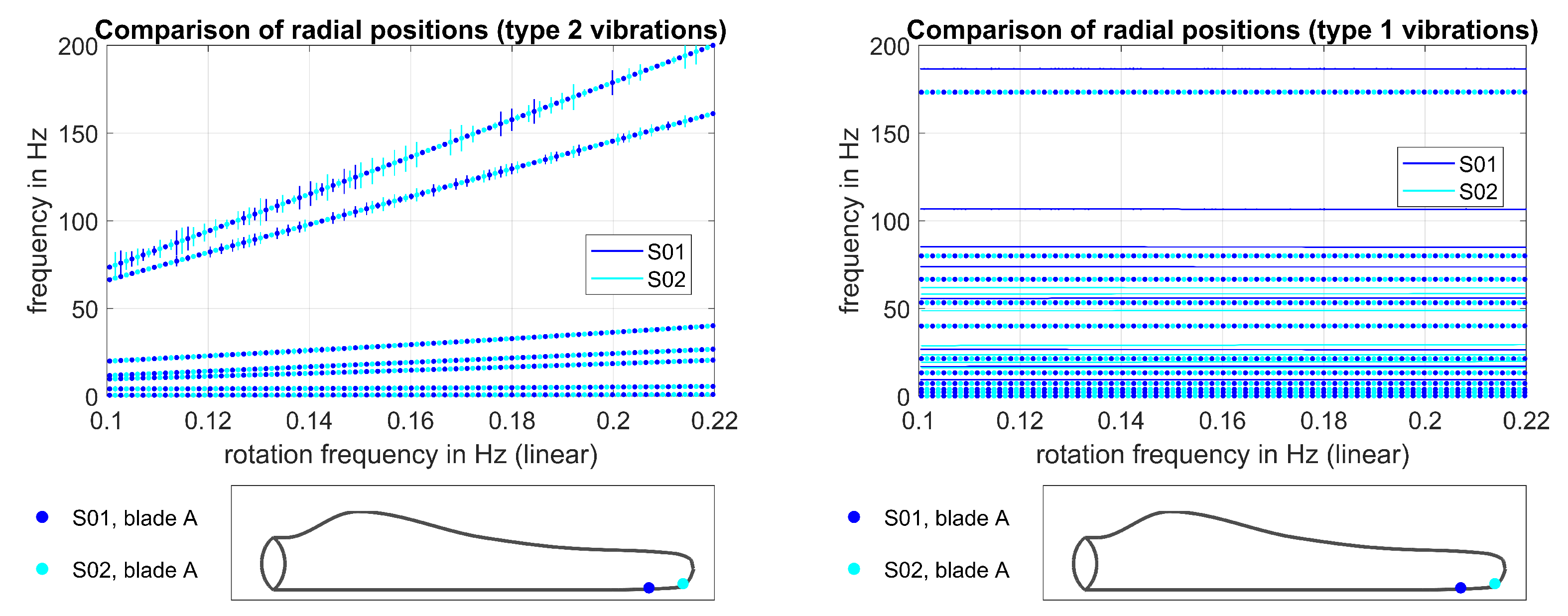
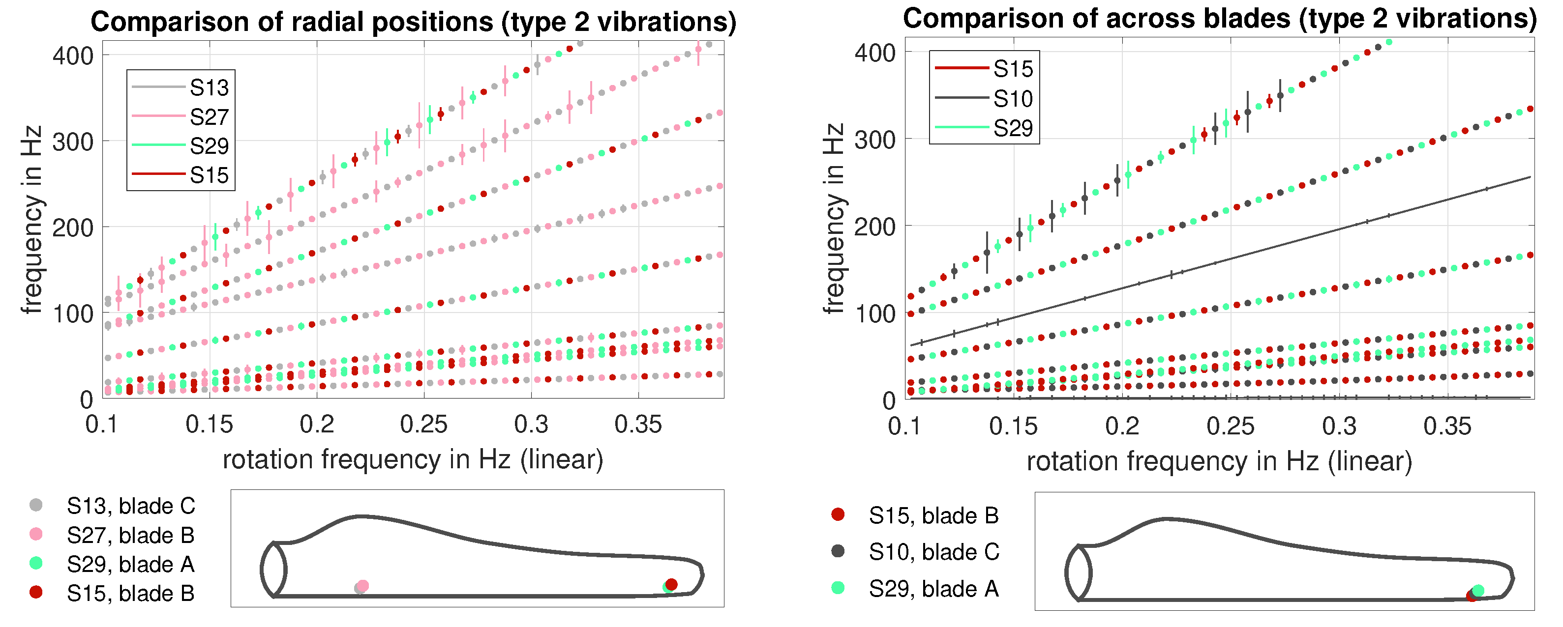
A comparison of sensors deployed at different radial positions along the blades is displayed in Figure 14 (left). Fingerprints of four sensors are visualised including two sensors mounted at the blade roots ( and ) and two sensors mounted at the blade tips ( and ) of Test Turbine 2. All sensors were mounted at the leading edge. Prominent Type 2 vibrations are reflected in the fingerprints of both root and tip sensors and correspond to global vibrations of the blade (see Vibrations 1, 3, 5 and 6 from the top). In addition, few vibrations were exclusively detected by Sensors and mounted the blade root (see Vibrations 2 and 4 from the top). Hence, fingerprints vary with the radial position of sensors, which corresponds to the extent of blade vibrations varying across radial positions due to the varying stiffness of the blade.
In addition, joint vibrations were detected in the lower part of spectrograms, i.e., Hz at Hz. However, regular block-wise gaps in data transmission increased noise especially in the lower frequency range. Therefore, assessing those vibrations is challenging and similarities or differences in fingerprints may be caused by data impurities and not by physical principles.
4.2.2. Comparison of Different Blades (Same Turbine Type)
Next, the effect of different turbine blades was evaluated by comparing sensors mounted at same positions but different blades. Each of Sensors , and was mounted at one blade tip of Test Turbine 2 (see Figure 14, right). Fingerprints of Sensors and on Blades A and B overlap, i.e., all identified vibrations in the mid to high frequency range were detected by both sensors. In contrast, the fingerprint of Sensor (Blade C) slightly deviates and an additional vibration was detected (see Vibration 3 from the top for Sensor ). A conclusion in favour of either a high sensitivity to measurement noise or different physical properties of Blade C is difficult due to the small size of the dataset. Besides the one additional vibration, characteristics of identified fingerprints overlap and indicate that there is no significant difference in blade properties at the blade tip for this test turbine. Again, joint vibrations in the lower part of spectrograms are not considered in detail due to measurement noise.
4.2.3. Comparison of Different Blade Sides
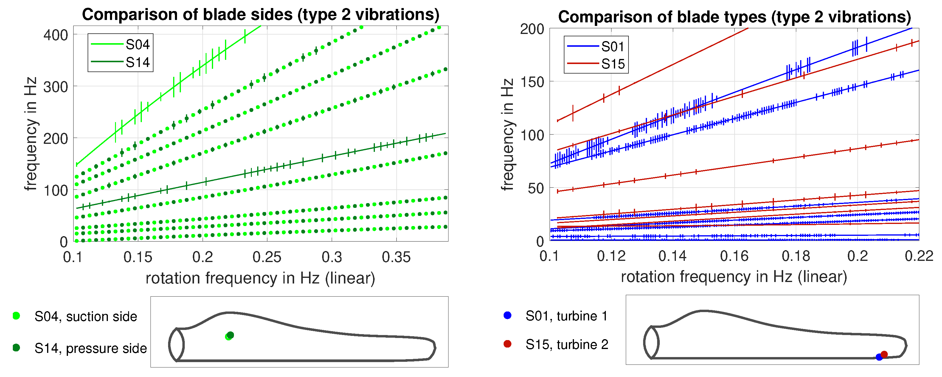
In addition, fingerprints were analysed for sensors mounted on different sides of the same blade, i.e., pressure side () and suction side () of Blade A of Test Turbine 2 (see Figure 15). Sensors were mounted at the same radial position at the blade root and at 50% distance to the trailing edge. The comparison of fingerprints shows that fingerprints overlap for most Type 2 vibrations. This indicates that the vibrational characteristic of the blade is very similar on both sides of the blade in the root section.
Differences can be noted for two vibrations: An additional vibration was detected by Sensor (fifth from the top) and covers a relatively large bandwidth in comparison to other vibrations in the same frequency range. This suggests that the vibration is not well-localised and is either nearly hidden in noise or falsely detected due to increased noise levels. In contrast, the second additional vibration detected by Sensor (first from the top) also shows a large bandwidth; however, it corresponds to other vibrations in the high frequency range, e.g., see Sensors and . Hence, monitoring both sides of the blade is promising for evaluating changes in the stiffness of the blade and identifying weak spots for damage detection and prevention.
4.3. Analysis across Turbine Types
Finally, vibrational characteristics were compared for both test turbines by analysing fingerprints of Sensors and on the blade tips of Turbines 1 and 2, respectively. Fingerprints are displayed in Figure 15 for the joint frequency range 0– 200 and joint operational range 0.1– .
While fingerprints show similar properties for sensors on same blade type, e.g., a comparison of blade tips of Test Turbine 2 (see Figure 14, right), results strongly deviate for sensors mounted on the blade tips of different turbine types as displayed in Figure 15. For all detected Type 2 vibrations, the increase in frequency with the rotation frequency is significantly higher for Turbine 2 with shorter blade length (represented by Sensor , 70 rotor diameter) than for Turbine 1 with longer blade length (represented by Sensor , 63 blade length). Accordingly, no overlap of any Type 2 vibrations was detected. A detailed comparison for several sensor positions is not possible at the current state since Test Turbine 1 was only equipped with two sensors at the blade tip.
5. Discussion
In this study, we propose an algorithm for analysing distributed vibration measurements on wind turbine blades. By extracting so-called vibration-based fingerprints, dominant vibrations could be extracted from linear-scale spectrograms for subsequent analysis. The functioning of the algorithm was demonstrated by using the rotation frequency of the turbine as a reference variable; however, the algorithm can be applied to almost any environmental or operational condition.
Fingerprints were analysed across multiple positions on the blades by mounting wireless sensors on two wind turbines. For the first turbine, two sensors at the blade tip showed matching fingerprints with higher noise levels for the sensor mounted at larger radial distance. The results demonstrate that the vibration-based fingerprint algorithm successfully identifies eigenfrequencies, narrowband noise and vibrations strongly varying with the rotation frequency. In addition, the algorithm considers inhomogeneous changes so that partly overlapping vibrations can be extracted, e.g., eigenfrequencies and narrow-band vibrations with low and high operational variability, respectively.
For the second turbine, fingerprints were extracted at seven positions along the blade and showed different characteristics for sensors mounted at: (i) different radial positions; and (ii) different sides of the blade. However, those results can only be treated as indications since detection results were impaired by low averaging due to a small dataset and high noise levels due to transmission errors.
Hence, the following challenges in vibration-based monitoring can be summarised: First, data loss and (semi-)systematic transmission errors in wireless sensors decrease detection accuracy and, consequently, need to be avoided. For example, the detection of eigenfrequencies with small amplitudes may be impaired by increased noise levels. Second, sufficient measurements need to be collected during varying operational conditions to optimally separate reference variables, e.g., rotation frequency and temperature. Finally, algorithm parameters may need to be adjusted across turbine types for best performance but need to be fixed for turbines of the same type to enable comparability. Hence, it is planned to continue the measurement campaign on the second test turbine and evaluate fingerprints on larger datasets and with reference to further reference measurements, e.g., the blade temperature.
6. Conclusions
In wind energy, monitoring of structural health is essential to minimise blade loads and increase the energy capture per turbine. Blade vibrations need to be studied both at different positions along the blade and during operation of the turbine. Thereby, turbine settings can be optimised to decrease vibrations at relevant positions along the blade.
In our approach, we measure vibrations at multiple positions along the blade by mounting wireless sensors on the blade surface. We propose an algorithm for automatically extracting the vibrational characteristic of the blade from acceleration measurements. The algorithm was tested on two test turbines, and the results demonstrate that the algorithm successfully extracts eigenfrequencies, narrowband noise and vibrations. In addition, the results indicate different vibrational characteristics of the blade at different sensor positions but will need to be verified with further measurements. Overall, the advantages of the vibration-based fingerprint algorithm can be characterised as follows:
- Automated extraction of dominant vibrations (e.g., eigenfrequencies or narrow-band noise) from measured frequency spectra.
- Analysis with regard to operational or environmental conditions.
- Continuous monitoring to track changes in the vibrational characteristic during the lifetime of the blade.
- Comparison of fingerprints for several positions along the blade, e.g., to optimise sensor positions in further monitoring applications or to improve blade design.
These benefits were demonstrated by means of acceleration measurements on wind turbine blades. In addition, the algorithm is promising for additional sensor types and structural health monitoring applications, in which vibrations have to be analysed with regard to varying environmental or operational conditions. For this, algorithm parameters can easily be adapted to the properties of measurements. With respect to wind energy, our algorithm contributes to gain a detailed understanding of blade vibrations during operation of the turbine. By incorporating this knowledge into operational turbine settings for existing turbines and blade design for next-generation turbines, blade vibrations can be minimised, thereby reducing wear of the blades and preventing preliminary aging.
In future work, it is planned to mount sensors on further test turbines and analyse vibration-based fingerprints across various turbine types. In addition, the fingerprint algorithm shall be extended by alarm thresholds in case of non-optimal turbine settings.
Author Contributions
Conceptualisation, T.L. and A.B.; methodology, formal analysis, data curation and software, T.L.; validation, T.L. and A.B.; writing—original draft preparation, T.L.; writing—review and editing, T.L. and A.B.; visualisation, T.L.; supervision, A.B. All authors have read and agreed to the published version of the manuscript.
Funding
The authors received no external funding.
Institutional Review Board Statement
Not applicable.
Informed Consent Statement
Not applicable.
Data Availability Statement
The data presented in this study are available on request from the corresponding author.
Acknowledgments
Open Access Publication supported by the Open Access Publishing Fund of Graz University of Technology. The authors would like to thank the company eologix sensor technology for providing sensor data and equipment, and the company VERBUND for supporting sensor mounting on their turbine.
Conflicts of Interest
The authors declare no conflict of interest.
Abbreviations
| AI | Artificial intelligence |
| DC | Direct current |
| DFT | Discrete Fourier transform |
| MEMS | Micro-electro-mechanical system |
| SSE | Sum of squared errors |
| STFT | Short-time Fourier transform |
| UAV | Semi-autonomous unmanned aerial vehicle |
References
- Komusanac, I.; Brindley, G.; Fraile, D.; Ramirez, L. Wind Energy in Europe—2020 Statistics and the Outlook for 2021–2025; Technical Report; WindEurope: Brussels, Belgium, 2020. [Google Scholar]
- International Renewable Energy Agency (IRENA). Renewable Energy Technologies: Cost Analysis Series; Volume 1: Power Sector, Issues 5/5; International Renewable Energy Agency (IRENA): Abu Dhabi, United Arab Emirates, 2012. [Google Scholar]
- Dao, C.; Kazemtabrizi, B.; Crabtree, C. Wind turbine reliability data review and impacts on levelised cost of energy. Wind Energy 2019, 22, 1848–1871. [Google Scholar] [CrossRef] [Green Version]
- Loss, T.; Bergmann, A. Moving Accelerometers to the Tip: Monitoring of Wind Turbine Blade Bending Using 3D Accelerometers and Model-Based Bending Shapes. Sensors 2020, 20, 5337. [Google Scholar] [CrossRef] [PubMed]
- Acar, G.D.; Feeny, B.F. Bend-bend-twist vibrations of a wind turbine blade. Wind Energy 2018, 21, 15–28. [Google Scholar] [CrossRef]
- Liu, H.; Zhang, Z.; Jia, H.; Li, Q.; Liu, Y.; Leng, J. A novel method to predict the stiffness evolution of in-service wind turbine blades based on deep learning models. Compos. Struct. 2020, 252, 112702. [Google Scholar] [CrossRef]
- Yoo, H.; Shin, S. Vibration analysis of rotating cantilever beams. J. Sound Vib. 1998, 212, 807–828. [Google Scholar] [CrossRef]
- Rafiee, M.; Nitzsche, F.; Labrosse, M. Dynamics, vibration and control of rotating composite beams and blades: A critical review. Thin-Walled Struct. 2017, 119, 795–819. [Google Scholar] [CrossRef]
- Khadka, A.; Fick, B.; Afshar, A.; Tavakoli, M.; Baqersad, J. Non-contact vibration monitoring of rotating wind turbines using a semi-autonomous UAV. Mech. Syst. Signal Process. 2020, 138, 106446. [Google Scholar] [CrossRef]
- Poozesh, P.; Sabato, A.; Sarrafi, A.; Niezrecki, C.; Avitabile, P.; Yarala, R. Multicamera measurement system to evaluate the dynamic response of utility-scale wind turbine blades. Wind Energy 2020, 23, 1619–1639. [Google Scholar] [CrossRef]
- Ou, Y.; Tatsis, K.E.; Dertimanis, V.K.; Spiridonakos, M.D.; Chatzi, E.N. Vibration-based monitoring of a small-scale wind turbine blade under varying climate conditions. Part I: An experimental benchmark. Struct. Control. Health Monit. 2020, 28, e2660. [Google Scholar] [CrossRef]
- Tcherniak, D.; Mølgaard, L.L. Vibration-based SHM system: Application to wind turbine blades. J. Phys. Conf. Ser. 2015, 628, 012072. [Google Scholar] [CrossRef] [Green Version]
- Tcherniak, D.; Mølgaard, L.L. Active vibration-based SHM system: Demonstration on an operating Vestas V27 wind turbine. In Proceedings of the 8th European Workshop On Structural Health Monitoring (EWSHM 2016), Bilbao, Spain, 5–8 July 2016. [Google Scholar]
- García, D.; Tcherniak, D. An experimental study on the data-driven structural health monitoring of large wind turbine blades using a single accelerometer and actuator. Mech. Syst. Signal Process. 2019, 127, 102–119. [Google Scholar] [CrossRef] [Green Version]
- Bull, T.; Ulriksen, M.D.; Tcherniak, D. The effect of environmental and operational variabilities on damage detection in wind turbine blades. In Proceedings of the 9th European Workshop on Structural Health Monitoring, Manchester, UK, 10–13 July 2018. [Google Scholar]
- Al-Khudairi, O.; Hadavinia, H.; Little, C.; Gillmore, G.; Greaves, P.; Dyer, K. Full-scale fatigue testing of a wind turbine blade in flapwise direction and examining the effect of crack propagation on the blade performance. Materials 2017, 10, 1152. [Google Scholar] [CrossRef] [PubMed] [Green Version]
- Sun, S.; Przystupa, K.; Wei, M.; Yu, H.; Ye, Z.; Kochan, O. Fast bearing fault diagnosis of rolling element using Lévy Moth-Flame optimization algorithm and Naive Bayes. Eksploat. Niezawodn. Maint. Reliab. 2020, 22, 730–740. [Google Scholar] [CrossRef]
- Liu, Z.; Zhang, L.; Carrasco, J. Vibration analysis for large-scale wind turbine blade bearing fault detection with an empirical wavelet thresholding method. Renew. Energy 2020, 146, 99–110. [Google Scholar] [CrossRef]
- Kumar, A.; Vashishtha, G.; Gandhi, C.P.; Zhou, Y.; Glowacz, A.; Xiang, J. Novel Convolutional Neural Network (NCNN) for the Diagnosis of Bearing Defects in Rotary Machinery. IEEE Trans. Instrum. Meas. 2021, 70, 1–10. [Google Scholar] [CrossRef]
- Yang, J.; Yang, F.; Zhou, Y.; Wang, D.; Li, R.; Wang, G.; Chen, W. A data-driven structural damage detection framework based on parallel convolutional neural network and bidirectional gated recurrent unit. Inf. Sci. 2021, 566, 103–117. [Google Scholar] [CrossRef]
- Yuan, F.G.; Zargar, S.A.; Chen, Q.; Wang, S. Machine learning for structural health monitoring: Challenges and opportunities. In Sensors and Smart Structures Technologies for Civil, Mechanical, and Aerospace Systems 2020; Huang, H., Ed.; International Society for Optics and Photonics, SPIE: Bellingham, WA, USA, 2020; Volume 11379, pp. 1–23. [Google Scholar]
- Cooperman, A.; Martinez, M. Load Monitoring for Active Control of Wind Turbines. Renew. Sustain. Energy Rev. 2015, 41, 189–201. [Google Scholar] [CrossRef]
- Manhertz, G.; Modok, D.; Bereczky, Á. Evaluation of short-time fourier-transformation spectrograms derived from the vibration measurement of internal-combustion engines. In Proceedings of the 2016 IEEE International Power Electronics and Motion Control Conference (PEMC), Varna, Bulgaria, 25–30 September 2016; pp. 812–817. [Google Scholar]
- Manhertz, G.; Bereczky, A. STFT spectrogram based hybrid evaluation method for rotating machine transient vibration analysis. Mech. Syst. Signal Process. 2021, 154, 107583. [Google Scholar] [CrossRef]
- Eologix Sensor Technology. Available online: https://www.eologix.com/en/solutions/windenergy/ (accessed on 8 December 2020).
Figure 1.
Proposed approach: The local vibration characteristic of the blade is measured by distributed sensors on the blade (left). Vibration measurements (middle) are used to extract characteristic fingerprints with reference to a reference variable, e.g., rotation speed (right).
Figure 1.
Proposed approach: The local vibration characteristic of the blade is measured by distributed sensors on the blade (left). Vibration measurements (middle) are used to extract characteristic fingerprints with reference to a reference variable, e.g., rotation speed (right).

Figure 2.
(Left) Exemplary sensor mounting on the outside of the blade during construction of a wind turbine. (Right) Demonstration of flexible sensor layout.
Figure 2.
(Left) Exemplary sensor mounting on the outside of the blade during construction of a wind turbine. (Right) Demonstration of flexible sensor layout.

Figure 3.
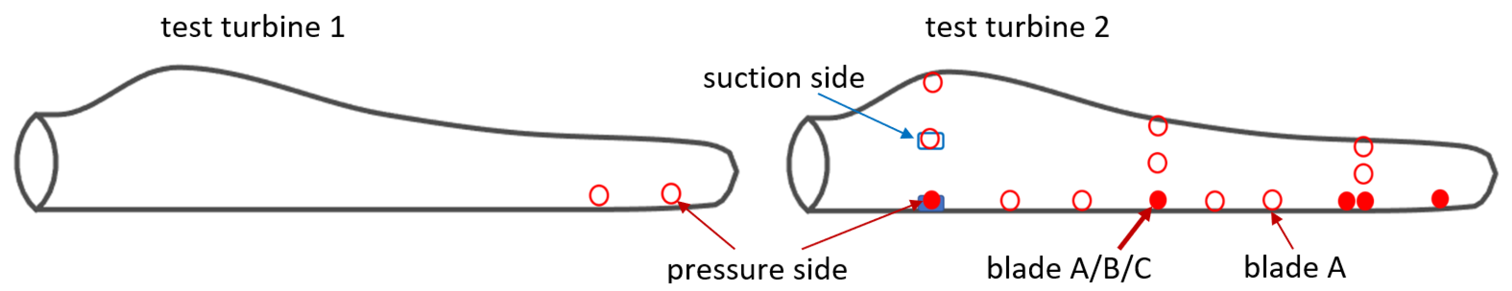
(Left) Sensor positions of Sensors S1 and S2 on Test Turbine 1. (Right) Sensor positions of Sensors S3–S23 on Test Turbine 2. Positions are marked with red circles and blue rectangles for positions on pressure side and suction side, respectively. Marker faces are solid for sensors deployed on all three blades and blank for sensors only deployed on the first blade (Blade A). Allocation of sensor numbers and positions displayed with results in the remainder of this paper.
Figure 3.
(Left) Sensor positions of Sensors S1 and S2 on Test Turbine 1. (Right) Sensor positions of Sensors S3–S23 on Test Turbine 2. Positions are marked with red circles and blue rectangles for positions on pressure side and suction side, respectively. Marker faces are solid for sensors deployed on all three blades and blank for sensors only deployed on the first blade (Blade A). Allocation of sensor numbers and positions displayed with results in the remainder of this paper.

Figure 4.
Overview of the proposed fingerprint algorithm in six analysis steps. Processing blocks are visualised for each step and presented in the corresponding sections.
Figure 4.
Overview of the proposed fingerprint algorithm in six analysis steps. Processing blocks are visualised for each step and presented in the corresponding sections.

Figure 5.
(Left) Exemplary triaxial measurement and corresponding vector sum displayed in the time domain, . Acceleration measured at 400 Hz and denoted with reference to gravitational acceleration (1 g = /). (Right) Single-sided power spectrum S(k) for the exemplary measurement, computed from the vector sum .

Figure 6.
Processing for an exemplary sensor with 400 Hz and the rotation frequency selected as reference variable. (Left) Non-linear-scale spectrogram with single measurement campaigns. (Middle) Linear-scale spectrogram with linear grid of size . (Right) Peak detection with peaks per grid point, peak assignment to Type 1 vibrations (), noise () and peaks used for detecting Type 2 vibrations () as discussed in the subsequent analysis. Colours of spectrograms corresponding to amplitudes on a logarithmic scale.

Figure 7.
Detection of Type 1 vibrations: (Left) Linear-scale spectrogram with identified peaks visualised; and (right) cumulative prominence of identified peaks with highlighted locations corresponding to locations of identified Type 1 vibrations.
Figure 7.
Detection of Type 1 vibrations: (Left) Linear-scale spectrogram with identified peaks visualised; and (right) cumulative prominence of identified peaks with highlighted locations corresponding to locations of identified Type 1 vibrations.

Figure 8.
Visualisation of vibration scanning and vibration filtering for detecting Type 2 vibrations.
Figure 8.
Visualisation of vibration scanning and vibration filtering for detecting Type 2 vibrations.

Figure 9.
Vibration scanning for detecting Type 2 vibrations. Peaks related to Type 2 vibrations displayed as samples with x and y axes normalised to [0,1]. (Left) Exemplary fitting for first-degree polynomial and second-degree polynomial and corresponding ranges and . (Right) Models corresponding to Type 2 vibrations for vibrations .

Figure 10.
Refinement of detected Type 2 vibrations by using 2nd degree models, examples shown for vibration (left) and (right) of an exemplary sensor. Model range was identified by using vibration scanning and vibration filtering, as described in Figure 8. Robust fitting with spectrogram amplitudes was used as weights, with coloured areas within range corresponding to non-zero weights.

Figure 11.
Fingerprint results for Sensors S1 (top) and S2 (bottom) mounted on the blade tip of test turbine 1. (Left) Linear-scale spectrogram with colour corresponding to logarithmic amplitude. (Middle) Extracted fingerprints, both Type 1 () and Type 2 () vibrations displayed. (Right) Sensor positions on the blade.

Figure 12.
Fingerprint comparison for Sensors S1 and S2. Separate visualisation for Type 1 (left) and Type 2 (right) vibrations. Solid lines represent vibrations only occurring in the fingerprint of one sensor, while dotted multi-coloured lines represent vibrations occurring jointly in both fingerprints. Error bars show locations of associated peaks with their length representing peak prominence.

Figure 13.
Fingerprint results for Sensors (top) and (bottom) mounted on tip and root of the same blade on Turbine 2. (Left) Linear-scale spectrogram with colour corresponding to logarithmic amplitude. (Middle) Extracted fingerprints, both Type 1 and Type 2 vibrations displayed. (Right) Sensor positions on the blade.

Figure 14.
(Left) Fingerprint comparison for Sensors , , and with varying radial positions on Turbine 2. (Right) Fingerprint comparison for sensors mounted on the blade tips of all three blades of Turbine 2 (, and ). Solid lines represent vibrations only occurring in the fingerprint of one sensor, dotted multi-coloured lines represent vibrations occurring jointly in multiple fingerprints. Error bars show locations of associated peaks with their length representing peak prominence.

Figure 15.
(Left) Fingerprint comparison for sensors on pressure side () and suction side () on the same blade and radial position (Blade A, Test Turbine 2). (Right) Comparison for tip sensors on Test Turbine 1 () and Test Turbine 2 (). Solid lines represent vibrations of a single sensor, dotted multi-coloured lines represent jointly occurring vibrations. Error bars show locations of associated peaks with their length representing peak prominence.


Table 1.
Parameters of the fingerprint algorithm for sensors on Test Turbines 1 and 2.
| Processing | Parameter | Turbine 1 | Turbine 2 | |||
|---|---|---|---|---|---|---|
| Spectrum Averaging | 163 (S2), 109 (S2) | 58 | ||||
| 1640 (S1), 1100 (S2) | 141–170 | |||||
| 7 × 10 | 5 × 10 | |||||
| 1 × 10 | 1 × 10 | |||||
| 2.2 × 10 | 3.9 × 10 | |||||
| Peak Detect. | 3.3 × 10 | 2.5 × 10 | ||||
| Type 1 Vib. | 1 × 10 | 5 × 10 | ||||
| Denoising | 3.3 × 10 | 2.5 × 10 | ||||
| Type 2 Vib. | 0 | 0 | 0 | 1.5 × 10 | 2.5 × 10 | |
| 3 × 10 | 5 × 10 | 1.5 × 10 | 2.5 × 10 | 5 × 10 | ||
| 5 × 10 | 2 × 10 | 1 × 10 | 2 × 10 | 2 × 10 | ||
| 0 | 0 | |||||
| 8 × 10 | 1.4 | |||||
| 1 × 10 | 1 × 10 | |||||
| 100 | 46 | |||||
| 4 × 10 | 8 × 10 | 5 × 10 | ||||
| , | 2 × 10 | 4 × 10 | 8 × 10 | 1 × 10 | 2.2 × 10 | |
| condition | strict | strict | strict | interval | interval | |
| 0 | 7.5 × 10 | |||||
| 1 | 1 | |||||
| 10 | 10 | 10 | 10 | 5 | ||
| 5 × 10 | 2 × 10 | 5 × 10 | 1 × 10 | 3 × 10 | ||
Publisher’s Note: MDPI stays neutral with regard to jurisdictional claims in published maps and institutional affiliations. |
© 2021 by the authors. Licensee MDPI, Basel, Switzerland. This article is an open access article distributed under the terms and conditions of the Creative Commons Attribution (CC BY) license (https://creativecommons.org/licenses/by/4.0/).
Share and Cite
MDPI and ACS Style
Loss, T.; Bergmann, A. Vibration-Based Fingerprint Algorithm for Structural Health Monitoring of Wind Turbine Blades. Appl. Sci. 2021, 11, 4294. https://0-doi-org.brum.beds.ac.uk/10.3390/app11094294
AMA Style
Loss T, Bergmann A. Vibration-Based Fingerprint Algorithm for Structural Health Monitoring of Wind Turbine Blades. Applied Sciences. 2021; 11(9):4294. https://0-doi-org.brum.beds.ac.uk/10.3390/app11094294
Chicago/Turabian StyleLoss, Theresa, and Alexander Bergmann. 2021. "Vibration-Based Fingerprint Algorithm for Structural Health Monitoring of Wind Turbine Blades" Applied Sciences 11, no. 9: 4294. https://0-doi-org.brum.beds.ac.uk/10.3390/app11094294
Note that from the first issue of 2016, this journal uses article numbers instead of page numbers. See further details here.