
Inertial Parameter Identification in Robotics: A Survey
by
 , , , and
Quentin Leboutet
1,* ,
,
Julien Roux
2,
Alexandre Janot
3,
Julio Rogelio Guadarrama-Olvera
1 and
Gordon Cheng
1 1
Institute for Cognitive Systems, Technical University of Munich, Arcistrasse 21, 80333 Munich, Germany
2
LIRMM, Université de Montpellier, 34095 Montpellier, France
3
ONERA the French Aerospacelab, 6, Chemin de la Vauve aux Granges, 91123 Palaiseau, France
*
Author to whom correspondence should be addressed.
Appl. Sci. 2021, 11(9), 4303; https://0-doi-org.brum.beds.ac.uk/10.3390/app11094303
Submission received: 11 April 2021
/
Revised: 29 April 2021
/
Accepted: 5 May 2021
/
Published: 10 May 2021
(This article belongs to the Special Issue Robots Dynamics: Application and Control)
Abstract
:This work aims at reviewing, analyzing and comparing a range of state-of-the-art approaches to inertial parameter identification in the context of robotics. We introduce “BIRDy (Benchmark for Identification of Robot Dynamics)”, an open-source Matlab toolbox, allowing a systematic and formal performance assessment of the considered identification algorithms on either simulated or real serial robot manipulators. Seventeen of the most widely used approaches found in the scientific literature are implemented and compared to each other, namely: the Inverse Dynamic Identification Model with Ordinary, Weighted, Iteratively Reweighted and Total Least-Squares (IDIM-OLS, -WLS, -IRLS, -TLS); the Instrumental Variables method (IDIM-IV), the Maximum Likelihood (ML) method; the Direct and Inverse Dynamic Identification Model approach (DIDIM); the Closed-Loop Output Error (CLOE) method; the Closed-Loop Input Error (CLIE) method; the Direct Dynamic Identification Model with Nonlinear Kalman Filtering (DDIM-NKF), the Adaline Neural Network (AdaNN), the Hopfield-Tank Recurrent Neural Network (HTRNN) and eventually a set of Physically Consistent (PC-) methods allowing the enforcement of parameter physicality using Semi-Definite Programming, namely the PC-IDIM-OLS, -WLS, -IRLS, PC-IDIM-IV, and PC-DIDIM. BIRDy is robot-agnostic and features a complete inertial parameter identification pipeline, from the generation of symbolic kinematic and dynamic models to the identification process itself. This includes functionalities for excitation trajectory computation as well as the collection and pre-processing of experiment data. In this work, the proposed methods are first evaluated in simulation, following a Monte Carlo scheme on models of the 6-DoF TX40 and RV2SQ industrial manipulators, before being tested on the real robot platforms. The robustness, precision, computational efficiency and context of application the different methods are investigated and discussed.
1. Introduction
1.1. Motivation and Related Works
The growing popularity of adaptive, predictive, and passivity-based control strategies in robotic applications raises new challenges for researchers and engineers. Since these methods rely on an explicit formulation of system dynamics, substantial research efforts are being made in the field of inertial parameter identification to improve their performance and robustness, see for example [1] and the references therein. In the context of rigid robots, techniques for identifying the inertial parameters are generally based on a rigorous analysis of joint movements and torque signals over a predefined time horizon. A given robot is tracking a trajectory that excites the different components of its dynamic model and the residuals in terms of motion and torque are used to refine the parameters estimates. The most common approach to offline or batch dynamic parameter identification is the Inverse Dynamic Identification Model with ordinary Least-Squares estimation (referred to as IDIM-OLS in [2,3]). This method is based on the assumption that the mapping between joint torques and the inertial parameters of a robot is linear (this holds provided that the robot links are rigid, that friction nonlinearity is negligible and that the joints are not subject to backlash). Both efficient and easy to implement, IDIM-OLS and its variants—including Weighted Least-Squares (IDIM-WLS) and Total Least-Squares (IDIM-TLS) methods described in [4]—however lack noise immunity and exhibit a strong dependence on the conditioning of the robot’s trajectory, as depicted in [5,6]. As a matter of fact, whether due to measurement noise, incorrect data-filtering, or insufficient excitation, IDIM-OLS parameter estimates may eventually prove to be highly biased, to the point of losing all physical coherence, yielding, for example, negative link masses, friction coefficients, or non-positive-definite rotational inertia. Over the past two decades, much research effort has focused on solving these issues, and multiple promising methods were proposed. These approaches can generally be divided into two distinct classes, whether the objective is to improve the statistical consistency of the estimates – physical consistency naturally stemming from statistical consistency (although the opposite is not true.)—or to more explicitly enforce physicality by means of dedicated constrained optimization techniques. In both cases, performance evaluation is generally carried out through direct comparison with unconstrained IDIM-OLS or IDIM-WLS. For instance, ref. [7] compared the performance of the IDIM-WLS method with that of an Extended Kalman Filter (EKF) estimator, on a 2 degree of freedom (DoF) SCARA robot. The results indicate that unlike IDIM-WLS, the EKF estimator has convergence issues and exhibits a strong dependence to both initial conditions and tuning parameters. In [8] the authors presented an approach based on Set Membership Uncertainty (SMU). This approach was tested on a 2 DoF SCARA robot and compared to IDIM-OLS but did not show significant improvement. In [9,10,11], the authors compared IDIM-WLS with a Maximum Likelihood (ML) estimator on 2- and 3 DoF robots. The results suggest that ML techniques may reduce the bias of the parameter estimates in the case of noisy joint measurements, at the price however, of a much greater computational effort. Interestingly, only a few studies have actually performed a formal comparison between more than two identification approaches at the same time, and on robots with many degrees of freedom, such as industrial manipulators or humanoids. In [5,12], the authors used a 6 DoF TX40 industrial robot manipulator to compare the Direct and Inverse Dynamic Identification Model (DIDIM) method, the Closed-Loop Output Error (CLOE) method, the Closed-Loop Input Error (CLIE) method and the IDIM-WLS. In [6] the same research team compared the Instrumental Variable approach (IDIM-IV) with IDIM-WLS, the Total Least-Squares approach (IDIM-TLS) and CLOE. The results suggest that DIDIM, IDIM-IV, CLOE and CLIE are significantly less sensitive to noise than Least-Squares approaches. The authors moreover enhanced the fact that DIDIM and IDIM-IV require much lower computational effort compared to CLOE and CLIE due to the reduced number of model evaluations. However, it is worth noting that DIDIM and IDIM-IV were not directly compared to each other. In [13,14], the authors compared five identification methods, namely the IDIM-OLS, Adaline Neural Networks (AdaNN), Hopfield-Tank Recurrent Neural Networks (HTRNN), EKF, and a genetic algorithm, on a 5-DoF SCARA robot. Among these five methods, only IDIM-OLS and AdaNN gave results that were accurate enough to be exploited. The results also suggest that other methods may lack regularity, as they do not converge for all the considered parameters. Recently, multiple works highlighted the possibility of explicitly enforcing physical consistency by means of constrained optimization techniques, rather than implicitly, through statistical consistency. With some notable exceptions (e.g., [15,16,17,18,19]), the classic approach to physically consistent parameter identification consists of expressing physicality constraints in the form of a Linear Matrix Inequality (LMI), thereby allowing the reformulation of the whole identification process as a constrained optimization problem, solvable using Semi-Definite Programming (SDP) methods, as for example proposed in [20,21,22,23], or using optimization on manifolds as proposed in [24,25,26]. Please note that although several approaches such as [27,28], use Deep Neural Networks (DNN) to learn the full robot dynamics, these contributions will not be considered in this work, as the mapping between DNN hyper-parameters and robot dynamic parameters is not yet fully understood, thereby making a comparison with conventional identification methods irrelevant.
1.2. Problem Formulation and Proposed Contributions
Although it seems possible from the previous studies to infer specific tendencies as to the performance and context of application of the different identification algorithms [29], it is worth noting that no study currently provides a general guideline, based on quantitative arguments, such as encoder noise level, sampling frequency or knowledge of the control law. To be valid, such a study should be carried out within the same framework, on a wide range of methods, under well-defined experimental conditions and using a Monte Carlo analysis scheme to provide statistically significant results. Although benchmarking is common practice in the automatic control community—see e.g., [30,31,32] among others—it is less common in robotics, with some notable exceptions [33,34,35]. In practice, evaluating the performance of an identification method on a real system proves to be a difficult task since the latter can never be perfectly modeled. This is a direct consequence of the wide variety of complex physical phenomena—such as backlash or nonlinear friction—that have a significant influence on the system behavior while being relatively challenging to model. On the contrary, the identification of a simulated system allows a rigorous quantification of an algorithm’s performance since the characteristics and parameters of the simulated model are well known and can therefore be used as a reference. The simulation also makes it possible to highlight the influence of specific physical phenomena—e.g., joint friction or measurement noise—on the estimates’ quality. Therefore, our first contribution is to propose a dedicated framework, in the form of an open-source Matlab toolbox, which makes it possible to formally evaluate the performance of multiple identification algorithms on the same robot model and under the same conditions or assumptions. We use this benchmark to formally evaluate the performance of a set of algorithms among the most widely used offline computational approaches to robot dynamic parameter identification. These methods are the IDIM-LS (including the WLS, IRLS and TLS variants), ML, IDIM-IV, Output Error methods (CLOE, CLIE, DIDIM), the Extended Kalman Filter (EKF) as well as several of its Sigma-Point and Square-Root alternatives (SPKF), the Adaline Neural Network (AdaNN), the Hopfield-Tank Recurrent Neural Network (HTRNN) and finally a set of Semi-Definite Programming (SDP) approaches with Linear Matrix Inequalities to enforce physical consistency (PC-IDIM-OLS, PC-IDIM-WLS, PC-IDIM-IRLS, PC-DIDIM). The reader can find a summary of the evaluated identification methods in Appendix A Table A1. Though it is always interesting to formally compare different methodologies, the usefulness of such a comparison remains questionable if no conceptual relationship can ultimately be established between these approaches. For instance, stating that IDIM-IV or DIDIM outperforms IDIM-OLS in the case of improper data-filtering and/or too noisy data is not really helpful nor constructive for practitioners since this gain of robustness against noises is expected from IDIM-IV, and Output Error approaches. Instead, it is more interesting to show how the data-filtering helps IDIM-OLS to provide results that match those provided by IDIM-IV and Output Error approaches. Therefore, our second contribution is to establish some relationships between different methods to emphasize their similarities and differences. Finally, establishing relationships allows providing some guidelines to practitioners non-expert in robot identification to help them to choose an identification method among all the available approaches: this is the third and last contribution of this work. The paper is organized as follows: Section 2 provides a theoretical overview of how simulated robot modeling and control are achieved in the context of identification. Section 3, Section 4, Section 5, Section 6 and Section 7 provide a theoretical overview of each method, highlighting their differences, weak points and discussing the potential implications in terms of expected performance. In more detail, Section 3 discusses the IDIM-OLS, -WLS, and -IRLS identification approaches, and highlight their weaknesses. Section 4 introduces the IDIM-IV, and ML approaches, Section 5 and Section 6 respectively introduce the Input- and Output Error methods (CLOE, CLIE, and DIDIM) as well as a set of the alternative approaches based on nonlinear Kalman filtering and neural networks. Section 7 discusses the different approaches allowing the enforcement of physicality in the parameter identification process. Section 8 then describes the proposed benchmark, emphasizing its structure and the adopted conventions. The different experiments, and their results, are presented in Section 9 and discussed in Section 10. Finally, Section 11 provides a brief conclusion and opens perspectives for further developments of BIRDy.
2. Robot Modeling and Control in the Context of Parameter Identification
2.1. Inverse and Direct Dynamic Models
The inverse dynamic model (IDM) of a rigid serial robot manipulator with n-degrees-of-freedom relates the joint-space motion quantities , to the generalized forces applied to the system. The IDM can be derived using the Euler-Lagrange formalism (c.f. [36]), resulting in the following equation
where denotes the generalized inertia matrix, the Coriolis and centripetal effects matrix, the gravitational torque vector, and the friction vector. This equation is parameterized by the vector concatenating the standard dynamic parameters of each robot link j, expressed as
where are the elements of the inertia tensor of link j, expressed at the link origin , refers to inertia of the actuator and transmission system, is the link mass, , are the coordinates of the link Center-of-Mass in and are the corresponding first moments (c.f. [37]). Let be the vector that regroups the Coriolis, centripetal, gravitational and frictional effects, namely . The direct dynamic model (DDM), allowing calculation of the joint accelerations as a function of the joint positions , joint velocities , generalized forces and of the vector of dynamic parameters, can then be written as
From Equation (3), is it clear that the DDM is nonlinear with respect to the dynamic parameters and the robot’s state vector defined as . By contrast, the IDM has the interesting property of being linear in , and can thus be reformulated as
where denotes the closed-form expression of the Jacobian matrix of with respect to , often referred to as the model regressor. It is worth noting that the equality in Equation (4) only holds provided that the friction term is also linear with respect to the parameter vector (in case this is not verified (4) is only a first-order approximation of a potentially much more complex system). and that the vectors and are noise-free. Under these assumptions, dynamic parameters identification can be considered to be an inverse problem. Sampling (4) at multiple different time epochs along a given state trajectory results in an over-determined observation system of linear equations in , for which a unique solution can be derived provided that the system is not rank deficient. Note however that this latter point turns out to be hardly verifiable in practice.
2.2. Base Parameters and Identification Model
As explained in [2], the rank of the sampled observation system is function of two factors, namely the nature of the collected data samples, and the internal structure of the regressor matrix . Data rank deficiency of the observation system is a direct consequence of noisy or improper data samples that do not adequately excite the model parameters (i.e., that do not sufficiently reveal their influence on the system dynamics). This issue can most of the time be solved by having the robot track a trajectory that is specifically designed to excite the model parameters [38]. The other aspect of the problem lies in the fact that the intrinsic geometrical properties of robot manipulators naturally imply that some of the dynamic parameters within the vector simply cannot be identified, for having rigorously no influence on the actual robot motions whatever the followed trajectory. In the same manner, some parameters can only be identified jointly because of their combined influence on the system. From a formal point of view, these issues can be characterized as a structural rank deficiency of the regression matrix . To solve this issue, it is necessary to perform a set of column rearrangements within , eventually leading to the set of base parameters that are actually linear combinations of the standard parameters . Base inertial parameters are defined by [39,40] as the set of dynamic parameters which is sufficient to completely describe the–intrinsically constrained–dynamics of a robot mechanism. As exposed in [37], the base parameter vector can be obtained by performing a set of rearrangements in the symbolic expressions of (4) (note that in this context, some of the performed symbolic simplifications are only made possible using proximal DH convention). In [41], an alternative computation method was proposed based on Fourier series decomposition of the robot dynamic equations. Dedicated numerical methods based, for example, on QR decomposition can also be used. Consider the observation matrix constructed by stacking the samples of obtained from a randomly generated set of distinct joint values:
where for , , is an upper-triangular matrix of rank and is a permutation matrix chosen – by default – so that the diagonal values of are arranged in decreasing order. Denoting by and the first b and last columns of leads to
where and respectively denote the first b and the last columns of . Since is orthogonal, one can write
with and , yielding
and hence the corresponding non-bijective mapping between the base parameter vector and the standard parameter vector
Note that—as explained in [20]—a bijective map can still be defined between and as
in which case the inverse mapping is
The problem of robot identification can hence be formulated as estimating the value of such that the dynamic behavior of the model matches that of the actual robot while it is tracking a permanently exciting trajectory. It is worth noting that as some of the base parameters may only have a minor influence on the robot dynamics, they can be neglected in practice. Therefore, a reduced set of parameters, referred to as “essential” parameters in [42] can be identified but will not be considered in this work.
2.3. Control Strategy
Robots being double-integrator systems, they are naturally unstable in open-loop and must therefore be operated and identified in closed-loop. Since most electrically actuated robots use Direct Current (DC) or Brushless Direct Current (BLDC) motors, the control structure at the joint level usually consists of a cascade of PD or PID regulators, the position and velocity loops providing a reference for the current-torque loop (c.f. [37]). As pointed out in [12,43], provided that the low-level current loop has a sufficient bandwidth, (typically, above 500 Hz, which is usually verified on most Direct current (DC) or Brushless Direct Current (BLDC) actuators since the torque reference is adjusted at the PWM frequency, i.e., 16–40 kHz) and considering the linear mapping between the current and the torque within DC and BLDC motors, its transfer function can be expressed as a static gain in the characteristic frequency range of the rigid robot dynamics (typically, less than 10 Hz for industrial robots as explained in [12,43]). In the case of a PD controller, the resulting control torque applied to the robot can be then typically be computed as:
where , and are the diagonal drive, position and velocity gain matrices and is a feed-forward term (assumed to be zero in this work). Please note that the drive-gain matrix contains the combined influence of the static gains of the current amplifiers, gear ratios and electromagnetic motor torque constants , and can thus be written as (c.f. [43]).
3. Inverse Dynamic Identification Model (IDIM) and Least-Squares (LS) Estimation Methods
3.1. Ordinary, Weighted and Iteratively Reweighted Least-Squares (IDIM-OLS, -WLS, -IRLS)
Let be the closed-form expression of the Jacobian matrix of with respect to the vector of base parameters, obtained by column rearrangements of the robot regressor matrix following , with the permutation matrix defined in Section 2.2. Then (1) can be rewritten in the following form:
In practice, because of the uncertainties caused by measurement noises and modeling errors, the actual torque differs from by an error so that (17) becomes
Equation (18) represents the Inverse Dynamic Identification Model (IDIM) relation (c.f. [43] and the references therein). The IDIM is sampled at a rate f while the robot is tracking exciting trajectories during an experiment. For N collected samples, an over-determined linear system of equations and b unknowns is obtained
where is the sampled vector of ; is the sampled matrix of , referred to as observation matrix; and is the sampled vector of . For the sake of compactness, will be noted in the rest of this work. Please note that is here assumed to be serially uncorrelated, zero-mean and heteroskedastic, with a diagonal covariance matrix . This choice is justified in [6,44] by the fact that robots are nonlinear multi-input multi-output (MIMO) systems. The most popular approach to solving (19) consists of computing the weighted least-squares estimate and associated covariance matrix
The diagonal terms of can be evaluated from the ordinary least-squares solution of (19), following the guidelines of [2]
where denotes the IDIM-OLS sampled error vector for joint j. Note that a correlation between the measured joint torque signals will result in non-negligible off-diagonal terms in . However, these terms can still be estimated using for instance the method of [23]. This method is both simple to implement and computationally efficient. In addition, it was successfully applied to multiple existing systems such as cars [45], electrical motors [46] or compactors [47]. It is worth noting that the vulnerability of OLS and WLS to outliers can be addressed using a specific Huber estimator (c.f. [48,49]). This is referred to as the Iteratively Reweighted Least-Squares (IRLS) in [50]. The resulting IDIM-IRLS method takes the form of an iterative process, which consists of applying additional penalty to the outliers, in the form of a dedicated weight vector and a weight matrix for each iteration i, in order to eventually mitigate their contribution to the final result
where refers to the element-wise multiplication operator. Accordingly, the IDIM-IRLS estimate at iteration i is given by
The weight vector is updated following
where is the element-wise min operator and is a tailor-made weight function. The process is iterated until convergence of the weights. This method was successfully tested on robotic systems in [23,51]. It is critically important to note that the LS estimates in general, will be unbiased if and only if the observation matrix is uncorrelated with the error term , or in other words, that the following equality holds
Unfortunately, the presence of uncorrelated random components within the observation matrix does not allow this hypothesis to be validated in practice. Noise sensitivity is especially problematic in the context of robotic systems as the joint accelerations, obtained by double time differentiation of the noisy encoder data, often exhibit poor signal-to-noise ratio with multiple outliers. A workaround to this issue is to filter the joint measurement signals as suggested by [2] where a pragmatic and tailor-made data-filtering is proposed. Nevertheless, this requires the knowledge of the bandwidth of the position closed-loop and special attention due to the bias induced by the filter, see [7,43,52] for more details. It is worth noting that in the case of periodic excitation trajectory with a known characteristic frequency, it is possible to use Fourier analysis tools to perform frequency domain filtering as suggested in [11,53]. The other alternative is to use identification methods that are robust against a violation of (25).
3.2. Total Least-Squares (IDIM-TLS)
The issue of noisy observation matrix, can in theory, be tackled using Total Least-Squares (IDIM-TLS) approach. As exposed in [54,55], the TLS estimate can be computed using a singular value decomposition of the augmented matrix as
where and . Following [4,56], the covariance of the TLS estimate can be approximated as
where is the minimum non-zero singular value of . Only a few pieces of research actually explore the potential use of total least-squares in the context of robot dynamic parameters identification. In [6], the authors observed that the IDIM-TLS estimate is biased if the joint data are not suitably filtered. Moreover, they noted that although TLS convergence occurs with adequate data-filtering, it does not outperform ordinary and weighted least-squares. Motivated by [57,58], in [59] part 4.2.6, the author raised some general comments on the IDIM-TLS method and stressed that its disappointing performance can be explained by the fact that it is based on the hypothesis that the noises have all the same variances whereas this assumption is violated in the case of an improper data-filtering according to [60]. It would in fact be more appropriate to use the Generalized Total Least-Squares (GTLS) method popularized by Van Huffel and Vandewalle, [4,61]. However, to properly use the GTLS method, the covariance matrix of noises involved in must be known. Unfortunately, if such an information is easily accessible for linear systems, it is not for robots. Indeed, besides the noise amplification effect induced by the process of numerical time derivation of the joint angles—used for joint velocity and acceleration computation—the IDM involves nonlinear functions such as the sine, cosine, square or sign operators, making the calculation of this covariance matrix difficult, if not intractable. This comment explains the reason the TLS or GTLS methods are seldom employed in the context of robot identification (see e.g., [54,62]) whereas they are widely considered in signal processing, see e.g., [63] and the references therein.
4. The Instrumental Variables (IV) and Maximum Likelihood (ML) Approaches
4.1. Inverse Dynamics Identification Model (IDIM) and Instrumental Variables (IV)
First introduced by [64] in the context of econometrics, the Instrumental Variables (IV) approach to parameter identification consists of defining an instrument matrix such that
which means that is both well correlated with the observation matrix and uncorrelated with the error term , see e.g., [6,65,66]. In this case, one obtains
and the IV estimates given by
are consistent. The use of IV for identification of robotic systems is reported in several approaches (see for instance [6,52,67,68,69,70] and the references therein). The critical issue here lies in the construction of the instrument matrix fulfilling (28a) and (28b). In this context, an ideal candidate for the instrument matrix appears to be the observation matrix denoted filled with simulated data that are the outputs of an auxiliary model, [66]. As explained in [6], for robot identification, the auxiliary model is the direct dynamic model (DDM) which is simulated assuming the same controller and reference trajectories that the one applied to the actual robot (c.f. Figure 1), and using the IV estimate obtained at the previous iteration. This defines an iterative algorithm. At iteration i and time epoch , the vector of simulated joint accelerations is computed as
By successive numerical integration of (31) one can obtain the vector of joint simulated positions and velocities denoted , respectively, from which it is then possible to build the instrument matrix by stacking the regression matrices obtained from the samples of at each as
Assuming that there are no modeling errors, the simulated joint positions, velocities and accelerations tend to the noise-free estimates denoted , respectively, yielding
Please note that given by (33) naturally complies with the conditions (28a) and (28b). In [6,52,69,70] the IDIM-IV estimates are formulated in a weighted recursive manner as:
where is given by (32). Once the IDIM-IV method has converged, the covariance matrix of the IDIM-IV estimates is given by
It should be emphasized that the consistency of the close-loop simulation in IDIM-IV relies on the assumption that the controller of the real robot and that of the simulated robot are the same. A difference in the control strategy will result in a different command being issued for a given state, eventually resulting in a bias in the parameter estimate. The results of [6,52,59,69,70] suggest that the convergence of IDIM-IV method is more robust against noise than IDIM-OLS/-WLS/-TLS and also faster than Output Error methods presented later in this article (c.f. Section 5). It should be noted, however, that convergence is slower than IDIM-OLS since simulation of the DDM is required. More generally since both the IDM and DDM are calculated from Newton’s laws, it seems more natural to simulate the DDM to construct rather than computing the covariance matrix of noises involved in and . In [52,69] the authors proved that IDIM-IV gives excellent results provided that the low-level controller is well-identified. Nevertheless, the robustness against high noise levels have not yet been suitably investigated and would deserve deeper treatment.
4.2. Maximum Likelihood (ML) Identification Method
Investigated in [9,10,11], the Maximum Likelihood (ML) parameter identification algorithms aims at tackling the issue of noisy torque and joint angle measurements. These works are the first ones actually addressing the issue of noisy observation matrices. In [10], the authors present an improvement of the original ML approach presented in [9]. The ML criterion they adopt can be formulated as
where denotes the diagonal variance matrix of the sample (this allows in particular to account for the effects of time differentiation in the joint signal in terms of noise amplification), is the error at the torque sample defined in (19); and is the Jacobian matrix of this error relative to the measurement vector . Because involves the IDM, this ML approach can be called IDIM-ML. In the IDIM-ML approach, the authors suggest constructing the vector by averaging the original measurements of and over realizations. Then, is used to construct the following observation matrix denoted . It must be noticed that provided is big enough and the variances of the original measurements are finite, the Lyapunov criterion ensures that is close to a Gaussian distribution. Note also that it can be even further assumed that tends to the noise-free original measurements as grows and the noise level is reasonable which means that one has . Interestingly, this ML approach is somehow related with the IDIM-IV method developed in [6]. Indeed, the authors suggest building an instrumental matrix such that using simulated data and the IDM while in [10] the authors suggest constructing with . Furthermore, in [71], the author establishes some interesting relationships between IV and ML approaches. It is thus expected that IDIM-IV and ML approaches give similar results. However, in [9] a prewhitening process has been carried out to remove all the coloring and correlation of the measurement noise. Without this prewhitening process which can be connected with the use of the decimate filter, the statistical assumptions made on the noise may be violated making the ML approach potentially unable to provide consistent estimates. Furthermore, it should also be stressed that the joint torques in these approaches are measured via current-shunt monitors instead of being the outputs of low-level controllers as usually done in [42]. Therefore, if the ML method does not require the simulation of the DDM, it could prove more sensitive to noises and is more time-consuming than IDIM-IV is.
5. The Output Error (OE) and Input Error (IE) Identification Approaches
5.1. Closed-Loop Output Error (CLOE)
As indicated by its name, an Output Error method consists of finding the parameter vector that minimizes the value function defined as the squared L2-norm of the error between the output of a system to be identified and the output of its model (see [72,73] and the references therein)
In the case of a robot we define (resp. ). Please note that Cartesian space formulations of the error function are also possible, see for instance [74]. The minimization of (37) is a nonlinear LS-optimization problem solved by running iterative algorithms such as the gradient or Newton methods which are based on a first- or a second-order Taylor’s expansion of the value function . The unknown parameters are therefore updated iteratively so that the simulated model output fits the measured system output, with
where is the innovation vector at iteration i. Output Error identification can be carried out in Open-Loop or in Closed-Loop. However, robots being double-integrator systems, Open-Loop Output Error (OLOE) turn out to be seldom used in practice compared to Closed-Loop Output Error (CLOE) as it is highly sensitive to initial conditions (c.f. [43] for a more detailed discussion on the topic). In CLOE, the simulated data are obtained by integrating the DDM in (3) assuming the same control law for both the actual and simulated robots—without gain adjustments—and using the estimate of calculated at iteration . The general principle of the CLOE method is illustrated in Figure 2. Let the simulated joint positions be the model outputs. At time the error to be minimized is given by
Then, if a classical Gauss-Newton algorithm is chosen, after data sampling and data-filtering, the following over-determined system is obtained at iteration i:
where is the vector built from the sampling of ; is the matrix built from the sampling of , the Jacobian matrix of evaluated at ; and the term is the vector built from the sampling of the residuals of the Taylor series expansion. Then, , the LS estimate of at iteration i is calculated with (40). Please note that numerically computing the Jacobian with finite differences requires model simulations. Therefore, CLOE is expected to be computationally expensive compared to IDIM-OLS or IDIM-IV. Once CLOE has converged, the covariance matrix of the CLOE estimates is given by
where is the variance matrix of the joint position measurement noise. Although CLOE is less sensitive to initial conditions, it turns out to be less responsive to changes in the parameters as explained in [5]. As a result, CLOE is expected to converge slowly and potentially to local minima. Please note that alternative optimization methods using the derivative-free Nelder–Mead nonlinear simplex method, Genetic Algorithm (GA), Particle Swarm Optimization (PSO) can potentially be used to tackle this issue. In [5] for example, the authors used the fminsearch Matlab function which makes use of the Nelder–Mead simplex algorithm. According to the results presented in [5], although the simplex method appears to be more robust than the classic Levenberg–Marquardt method, it requires an even higher computational effort.
5.2. Closed-Loop Input Error (CLIE)
The CLIE method can be seen as a variation of the CLOE method where the simulated torque is being used instead of the simulated position in Equation (37), resulting in and . The general principle of the CLIE method is illustrated in Figure 3. In this case, the error function which must be minimized at time has the following expression
and relation (40) thus becomes
where is the vector built from the sampling of ; is the matrix built from the sampling of , the Jacobian matrix of evaluated at (often referred to as input sensitivity); and is the vector built from the sampling of the residuals of the Taylor series expansion. Then, , the LS estimate of at iteration i is calculated with (43). Once CLIE has converged, the covariance matrix of the estimate is given by
This method was successfully implemented in [12] and formally compared to CLOE, DIDIM and IDIM-OLS. From this work, it appears that although CLIE outperforms both IDIM-OLS and CLOE in terms of accuracy, it has a similar computational complexity as CLOE, as a direct consequence of the finite difference Jacobian matrix computation. The authors demonstrated that CLIE could in fact be thought of as a frequency weighting of the CLOE method by the controller’s gains. This property can be verified in practice by re-injecting (16) into the expression of the sensitivity matrix . As a result, although the two estimators are asymptotically equivalent, CLIE proves in practice to be more sensitive to the changes in parameters than CLOE, thereby inducing better convergence properties.
5.3. The Direct and Inverse Dynamic Identification Model (DIDIM) Algorithm
In [43], a new algorithm termed Direct and Inverse Dynamic Identification Model (DIDIM) was proposed. The DIDIM method can be seen as a variation of the CLIE algorithm where some judicious approximations, made in the torque Jacobian matrix computation, yield . The initial nonlinear LS problem at iteration i hence turns into a much simpler linear LS problem allowing the DIDIM estimates to be calculated as
where is the observation matrix constructed with the joint simulated position, joint velocities and joint acceleration obtained from the closed-loop simulation of the DDM with as explained in Section 4.1. The general principle of DIDIM is illustrated in Figure 4. Once DIDIM method has converged, the covariance matrix of the DIDIM estimates is given by
According to the results gathered in [12,43,75], the DIDIM algorithm converges significantly faster than the CLOE and CLIE methods as it only requires a single robot simulation per iteration. In [12], the authors also demonstrate that DIDIM has a similar precision as CLIE. It is interesting to note that the OE methods are generally less sensitive to noise than IDIM-OLS methods since only simulated data are used to build . Until now, no formal comparison with IDIM-IV was carried out although [76] provides some elements of discussion, suggesting that the two methods have similar performance. However, further investigations must be conducted to refine the conclusions made in [76].
6. Direct Dynamics Identification Model (DDIM) with Nonlinear Kalman Filtering (NKF) and Neural Networks (NN) Methods
6.1. Direct Dynamics Identification Model (DDIM) and Nonlinear Kalman Filtering (NKF)
Widely used for state estimation purpose, Kalman filtering techniques can also be exploited in the context of parameter identification. As explained in [77], identification can be carried out in two different manners, denoted respectively as dual method (c.f. [78,79]) and joint method (c.f. [7,14,80,81]). In the first approach, the system state and parameters are identified separately, within two concurrent Kalman filter instances, while in the second one, state and parameters are estimated simultaneously, within a single Kalman filter featuring an augmented state representation. With the notable exception of [79], approaches to robot dynamic parameters identification found in the scientific literature are usually based on the joint filtering paradigm. Since this approach allows accounting for the statistical coupling between the state and the parameters, as suggested by [82], it is, therefore, expected to be significantly more robust than the dual filtering method. In the joint filtering approach, at time , the state vector and the current estimate of base parameters are stacked column-wise into a higher-dimensional state vector resulting into the following set of update equations:
where is the process noise; is the measurement noise; , are respectively the process-noise and measurement-noise covariance matrices; is a selection matrix; denotes the identity matrix, and the zero matrix. As with [7], the nonlinear state transition function is given by the robot direct dynamic model (DDM) as
In [79], the authors used a different state representation, assuming that the noise level in the joint encoders was negligible, and that the joint motion derivatives could therefore be computed independently. In this context, the state update Equation (48) can be simplified into , with while the measurement prediction equation consists of the IDM, computed using the Recursive Newton Euler (RNE) algorithm (c.f. [83]). Note that this is not the exact formulation of [79], as the authors use sigmoid barrier functions to enforce physical consistency. This aspect is discussed in greater details in Section 7. In practice, the DDM nonlinearity in (47) and (48) can be addressed in several different manners. We here briefly present some of the most popular approaches, namely the Extended Kalman Filter (EKF), the Sigma-Point Kalman Filter (SPKF) and the Particle Filter (PF). In the EKF, the prior estimate is propagated through a first-order linearized version of the robot dynamics. Although the resulting computational cost is low, it should be noted that the first-order linearization induces a bias in the posterior mean and covariance of the estimate. This bias can be non-negligible when the considered system is highly nonlinear. In SPKF implementations such as the Unscented Kalman Filter (UKF) or the Central Difference Kalman Filter (CDKF), a set of deterministic samples of the prior estimate (assumed to be normally distributed) are propagated through the true nonlinear dynamics of the system. In this manner, the nonlinearities can be taken into account up to the second order. Although this method significantly reduces the bias on the estimates of the posterior mean and covariance, it must be noted that it has a higher computational cost than the EKF, although it remains on the same order of magnitude. This aspect is discussed in greater details in [82]. Finally, in a Particle Filter (PF) no prior assumption is made on the nature of the estimate distribution. The latter is in fact sampled using a Monte Carlo method, hence resulting in enhanced robustness, even to severe non-linearities and non-Gaussian noises, but at the expense of computational cost, as the number of particles has a direct influence on the precision of the estimate (c.f. [84,85]). The full derivation of the EKF, SPKF and PF algorithms being out of the scope of this paper, the reader is referred to [82] for a more in-depth discussion and comparison between the different filters. In the context of parameter identification, it is worth noting that in Equation (48a) may either denote the torque measured during the experiments—as is for example the case in [7,80]—or the control torque applied to the simulated closed-loop system during the time-update step of the Kalman filter. In this manner, parameter identification can still be achieved when torque measurements are not available or available at a low sampling rate, but that the robot control structure and control parameters are known. Note however that in the latter case the control loop is updated at the robot control frequency . As a result, several control iterations can potentially be executed between two updates of the Kalman filter. To the best of our knowledge, this was so far never applied to the field of parameter identification.
6.2. Parameter Identification Using an Adaline Neural Network (AdaNN)
The Adaline (ADAptive LInear NEuron) uses stochastic gradient learning to converge to the IDIM-OLS estimate. The estimator has the following dynamic equation
where is the error defined in Equation (18). The parameter estimate at epoch can hence be expressed recursively as
where is the observation matrix of the real system at epoch , is the corresponding torque, and is referred to as the learning rate. A single “neuron” thus allows full model identification (c.f. Figure 5a). As several passes over the hole dataset may be necessary to achieve proper convergence, the sequence of observations and must be randomly reshuffled to avoid cycles [86]. Applications of the Adaline method to robot identification was investigated in [13,14]. The results suggest that the main advantage of Adaline over IDIM-OLS could be its ability to run online.
6.3. Parameter Identification with Hopfield-Tank Recurrent Neural Networks (HTRNN)
Hopfield-Tank recurrent neural networks are dynamic systems made of a set of N interconnected units, or neurons. Each neuron i behaves as an integrator coupled with a specific nonlinear activation function f as depicted in Figure 5b. In its original formulation [87], the neuron continuous state equation is expressed as
where is the internal state of neuron i, is its input bias, is the connection weight of neuron i with neuron j, , and where are design parameters corresponding to a resistance and a capacitance respectively. As with [13,14,88] we consider in this work the discrete Abe’s formulation of Hopfield-Tank neural networks (originally described in [89]) since, as explained in [88,90], it is particularly suitable for parametric optimization and parameter identification purpose. In Abe’s formulation, the activation function is a hyperbolic tangent:
This leads to the following discrete neuron state equation:
where is a tuning parameter often referred to as the learning rate of the network. It can be demonstrated (c.f. [88,91]) that such a dynamic system is asymptotically Lyapunov-stable, and that its natural evolution converges toward the minimum of the following energy function:
where , and . Under these conditions, the process of parameter identification can be thought of as matching the L2-norm of the parameter error of Equation (19) with the energy function (Section 6.3) of the Hopfield network. This can be achieved by selecting:
The resulting neural network will therefore have as many neurons as base dynamic parameters to identify, and the corresponding parameter estimate will converge to the ordinary least-squares (IDIM-OLS) estimate, provided that the appropriate solution range is selected. This range should therefore be carefully adjusted. This is made possible by properly tuning the parameter in (53).
7. Enforcing Physical Consistency within Inertial Parameter Identification
7.1. Mathematical Formulation of the Physical Consistency Constraints within a Parameter Identification Process
The possibility of enforcing physical consistency as part of a parameter identification process has been the subject of extensive research over the past two decades, in robotics. Early contributions, such as [15,16,20], formulated the parameter physicality of a given robot link j, as a set of positivity constraints on its mass , viscous-Coulomb friction parameters and on its transmission-chain inertia , as well as a positivity-definition constraint on the inertia tensor expressed at the link’s CoM, namely
It is worth noting that prior [20], approaches to physically consistent inertial parameter identification were usually leveraging the equivalence between the positivity-definition constraint on the inertia matrix a set of strict positivity constraints on its eigenvalues and . These eigenvalues are in fact the moments of inertia along the so-called link’s principal axes of inertia, yielding
where and is the rotation matrix relating the frame of the principal axes of inertia, to the link’s Center-of-Mass frame . In this context, ref. [16] proposed a reformulation of IDIM-OLS as a nonlinearly constrained optimization problem, solved using Sequential Quadratic Programming (SQP), while [79] suggested to directly identify the elements of instead of , using sigmoid functions within an EKF identification loop to smoothly bound the parameter estimates to physicality. It is worth pointing that such an approach could also possibly be applied to the HTRNN identification process by modifying the hyperbolic tangent activation function, although, to the best of our knowledge, this was never done. Conversely, ref. [20] proposed reformulating IDIM-LS under physicality constraints in a Semi-Definite Programming (SDP) perspective, writing (56) in the form of a Linear Matrix inequality (LMI). Provided that the reference frame of link j and its CoM frame have the same orientation, can indeed be related to the inertia tensor expressed in , using the Huygens-Steiner theorem
where denotes the vector of link’s first moments and . Observing that (58) is in fact the Schur complement of a matrix allows rewriting (56) as
where respectively denote the zero and identity matrices. In [21,22,24], the authors went one step further by noticing that (56) and (59) could still potentially lead to inconsistent link mass distributions. They consequently defined a density-realizability criterion as an additional triangle-inequality condition to be fulfilled alongside with (56), namely
where denotes the trace operator. A reformulation of the term within the constraint matrix was eventually proposed to account for density realizability constraints alongside with (56)
Naturally leading to the following SDP reformulation of IDIM-OLS and -WLS, that will be here referred to as Physically Consistent (PC-IDIM-OLS and -WLS)
where denotes the inverse mapping defined in (15). It is worth mentioning that the very structure of IDIM-IRLS (c.f. [23]), IDIM-IV and DIDIM (c.f. [92]) also makes it possible to seamlessly integrate the LMI physicality constraints by actually solving an SDP at each iteration of the corresponding algorithms. For instance, the PC-DIDIM algorithm (proposed in [92]) can be implemented by solving at each iteration i
Please note that [19] recently proposed a set of alternative parametrizations, allowing direct enforcement of physicality of the reconstructed dynamic parameters without need for constrained optimization techniques. Following their method, one could for instance enforce the constraints in (61) by adopting the parametrization , based on the Cholesky decomposition of
where is the element of row i and column j of the lower triangular matrix and is a regularization term. It is also worth mentioning that [93] independently proposed a linearization of both the positivity-definition and density realizability constraints applied to , in the form of a mass-positivity constraint applied to a distribution of point-masses located within each robot link (this is not without reminding the linearized friction-cone constraints applied to walking robots to ensure stable contacts with the environment). Provided that the number of point-masses is “high enough”, PC-IDIM-OLS and -WLS can be reformulated as Quadratic Programs (QP) with a good precision. Nevertheless, although QP are generally extremely fast to resolve, dimensionality can here rapidly become problematic since a good approximation of a link mass distribution typically requires several hundreds of samples.
7.2. Preventing Marginal Physicality
As highlighted in [25,26], imposing parameter physicality using a set of rigid constraints within an optimization process may eventually lead to situations where the parameter estimates lie at the very border of the physical consistency spectrahedron. This phenomenon, referred to as marginal physicality, typically occurs when the unconstrained estimate lies outside the physicality region, as it might for instance, be the case when the observation matrix is ill-conditioned, due to a lack of excitation or to excessive noise in . In [16,94] for instance, the authors proposed adding a relaxation term within the IDIM-OLS cost function, minimizing the Euclidean distance between the current parameter estimate and the set of initial standard parameters of the robot. In this case, (62) would be reformulated as
where is a tuning quantity. In practice, this term allows “shifting” the current parameter estimates toward the CAD original estimates which, by essence, are physically consistent. Observing that the set of physically consistent parameters, verifying (61) could be given a Riemannian manifold structure, with a well-defined metric, refs. [25,26] proposed to replace the Euclidean distance used in the relaxation process by a non-Euclidean distance, eventually leading to
where refers to a distance function on the set of physically consistent parameters.
8. Introducing the BIRDy Matlab Toolbox: A Benchmark for Identification of Robot Dynamics
In this work, we conduct a rigorous and systematic performance analysis of the different algorithms described above. This analysis is carried out within a single framework and on the same robot models, following a Monte Carlo process to ensure the statistical relevance of our results. Our main objective is ultimately to provide a set of general guidelines as to the applicability of a given identification method to a particular experimental context. To our knowledge, no comparison has been made to date on such a scale, although several identification frameworks are already available [33,34,35]. To ensure the repeatability of our results and their generalization to different robot models or experimental conditions, we propose a new open-source identification framework in the form of a dedicated Matlab toolbox named BIRDy (i.e., Benchmark for Identification of Robot Dynamics). BIRDy offers a wide range of functionalities, allowing the end-user to simulate, debug and identify his own robots while focusing on the mathematical aspects of identification rather than on the implementation of his own experimental framework. As observed by [53,95], offline parameter identification methods often follow a similar workflow, whose main steps usually involve:
- 1.
- selecting an appropriate model for the studied system,
- 2.
- designing a state trajectory which excites the different components of this model,
- 3.
- collecting a bunch of experimental data by having the—real or simulated—system follow the generated excitation trajectory,
- 4.
- executing the selected identification process,
- 5.
- evaluating the quality of the results by comparing the predicted and actual torques along a validation trajectory.
The very structure of BIRDy is directly inspired by this pipeline of operation (c.f. Figure 6). The various aspects of this configuration are presented and discussed in the following subsections, along with their operation modalities.
8.1. Symbolic Model Generation
Model generation is the very first step toward identification: not only should the robot be simulated in a realistic manner, but its dynamics should also be expressed in the form of a system of linear equations (c.f. Equation (17)) with a well-conditioned identification regressor. BIRDy features a symbolic model generation engine, capable of computing the complete kinematics, dynamics and identification models of any fixed-base serial robot. The cases of parallel robots—such as Stewart platforms—or floating-base robots—such as Humanoids—are not yet implemented in this approach and are here considered to be future works. Similar to the robotic-system-toolbox proposed by [96], the simulated robots are described using dedicated parameter files, containing a Denavit–Hartenberg table as well as the corresponding reference dynamic, friction and control parameters of each link. Both classic (distal) and modified (proximal) Denavit–Hartenberg conventions are supported. The dynamic model is generated using the Euler-Lagrange equations of motion (c.f. [36]). It is worth noting that in case the robot is gear-driven, the inertia of the actuators and gearboxes can be precisely taken into account within (1) following the approach of [97]. A simpler alternative—used in BIRDy—consists of modeling the drive-chain inertia as an additional diagonal term within the inertia tensor , following the approach of [44]. The symbolic expression of the regressor matrix is computed following the approach detailed in [98]. Finally, the vector of base dynamic parameters and the corresponding identification regressor are generated numerically, following the QR decomposition method of [39] described in Section 2.2.
8.2. Trajectory Data Generation
To avoid data rank deficiency of the observation matrix , the different components of the model should be sufficiently excited during the experiments. This can be achieved by means of specific joint trajectories, referred to as exciting. The design of excitation trajectories has been widely investigated over the past two decades, see e.g., [9,17,23,38,53,99,100,101,102]. From these works, it appears that the conditioning of the observation matrix is a relevant quality indicator for the generated trajectory. In our case, joint trajectories are obtained by parametrization of finite Fourier series as presented in [9,23,101]. The following cost criterion is minimized over the experiment time horizon using a standard nonlinear programming solver (in our case the “fmincon” and “ga” Matlab functions):
where refers to the condition number of a matrix; is the smallest singular value of ; and are tuning gains defined by the user. It should be emphasized that this method also allows the generated trajectories to be constrained to comply with the physical limitations of the considered robot, such as joint, velocity, torque or operational space limits. The generated trajectory is eventually stored in a dedicated data container. We provide multiple interpolation routines, based on the “interp1” Matlab function, so that relevant trajectory data can be obtained at any epoch, from a limited number of points, either generated by the optimizer or coming from a pre-existing file, created outside BIRDy. Please note that any third-party trajectory file containing a time series of joint values can be imported into the benchmark, provided its data are first stored in one of its predefined data containers.
8.3. Experiment Data Generation and Pre-Processing
Identifying the dynamic parameters of a robot manipulator requires the collection of appropriate measurements in terms of joint angles and torques over a predefined time horizon. Such data can be collected when a robot—real or simulated—tracks an exciting trajectory. As depicted in Figure 6, BIRDy provides a set of simulation routines, allowing the previously generated robot models to be used for this purpose. The data collection process in the case of a simulated robot is depicted in Figure 7. The direct dynamic model (DDM) of the robot, computed according to Equation (3), is subjected to a control torque . BIRDy contains implementations of multiple friction models, in particular the Viscous-Coulomb, Stribeck and LuGre models, allowing for more realistic data generation (c.f. [103]). The resulting joint acceleration signal is integrated twice, using a fixed-step Runge–Kutta method (RK1, RK2 or RK4) before a zero-mean Gaussian noise with a standard deviation is added to it. The resulting signal is then derived and eventually fed back into the controller without filtering. This allows better accounting for the effects of the numerical differentiation process occurring on real digital controllers, in terms of amplification of the measurement noise. The control algorithm itself is described in Equation (16). The robot tracks the reference trajectory at an update frequency . The data sampling process occurs at a frequency , both for and for the torque measurement (namely the torque signal corrupted by a zero-mean Gaussian noise with a standard deviation ). Please note that the reference trajectory files created by BIRDy can also be used to generate desired behaviors directly on a real robot manipulator. However, in this case, the data collection process is achieved independently using the robot communication interface. Unlike the BIRDy simulation interface, which provides direct feedback in terms of joint position and torque, the real robot interface often provides feedback only in terms of joint position and drive currents . Nevertheless, a reliable prior knowledge of the robot drive gains of (16) makes it possible to reconstruct the torque signal . In practice, the robot drive gains can be identified following a dedicated Least-Squares method such as that proposed by [104,105]. The “raw” signals used for identification purpose, are eventually built from by sequential time derivation followed by a parallel-decimation step in order to eliminate torque ripple and high-frequency noise components. The term “raw” here refers to the fact that the signals used for identification are not necessarily filtered. This makes it possible to test the robustness of the different identification algorithms to measurement or numerical differentiation noise. The parallel-decimation process in BIRDy is carried out with a zero-shift low-pass Tchebyshef filter, implemented using the decimate Matlab function. Similar to [2,6] the cutoff frequency is set to be approximately one order of magnitude higher than the joint bandwidths. The decimation ratio by which the input data are being sub-sampled is defined as where f is the sampling frequency. As additional band-pass filtering may be required by some algorithms (such as IDIM-OLS), the pre-processing pipeline of BIRDy also features an implementation of zero-shift Butterworth filter that can potentially be applied to the raw joint position signal before time derivation.
9. Benchmarking Inertial Parameter Identification Algorithms: Monte Carlo Simulations and Validation Using BIRDy
9.1. Hardware Description and Experiment Setup
This work takes the form of a case study, carried out on two different robots, both in simulation and on the real systems. These robots are the 6-DoF RV2SQ industrial manipulator from Mitsubishi, depicted in Figure 8b and the 6-DoF TX40 robot from Staubli, depicted in Figure 8a. Both are described using the proximal DH convention. Widely used for industrial and research purposes, these systems are ideal test platforms for having a similar kinematic structure but somewhat different communication interfaces and control characteristics. Generally speaking, evaluating the performance of multiple identification methods on different robot models within the same framework is relevant. It allows observing the influence of system-specific factors, such as the sampling rate or the control structure’s knowledge, on the overall algorithm performance. This, in turn, makes it possible to infer guidelines regarding the selection process of an identification algorithm depending on the experimental context. In practice, while the TX-40 has a high-speed communication interface allowing the joint position and torque to be sampled at rates of up to kHz, the data acquisition process on the RV2SQ is achieved at a much lower frequency, namely Hz. Moreover, although the low-level control characteristics of the TX40 are known with a sufficient level of accuracy (see in particular [6]), it must be emphasized that no prior knowledge of control structure, gains nor bandwidth of the RV2SQ is available. In this work, the low-level control structures are assumed to be of cascaded PD type—as described in Section 2.3—with a control bandwidth kHz. Please note that during the simulation experiments the control structure and gains used for data generation and identification are the same. Although hardly verifiable in practice, this hypothesis has critical implications as to the convergence properties of identification algorithms that are based on successive closed-loop DDM simulation runs such as DIDIM, CLIE, CLOE or NKF. We considered an integrated Viscous-Coulomb friction model for both data generation and parameter identification processes. This choice is deliberate and justified by the results exposed in [6,106]. In this model, the component of the friction force vector is expressed in the form of a linear function of two parameters, namely the Coulomb friction force and of the viscous friction coefficient as
As a result, the friction coefficients can be directly included within the link’s standard dynamic parameter vector , as shown in Equation (2).
A specificity of the TX40 is the coupling existing between the joints 5 and 6 of the robot. As explained in [75], this can be accounted for using two additional friction parameters denoted and . Although it was decided to neglect this coupling during the simulation experiments, this was later taken into account during the validation phase on the real robot. In the context of Monte Carlo Simulation (MCS) experiments, the model generation step resulted in a vector of 52 base dynamic parameters for each robot. During the validation experiments on the TX40, this base parameter vector was of dimension 54 due to and . It is worth noting that in the more general case where joint friction is nonlinear, provided that the friction model is not load dependent, the IDM given by (1) can be identified using a separable approach as suggested by [59,106]. The detail of such method being out of the scope of this paper, the reader is redirected to [107] and the references therein for a more detailed review of friction modeling and identification. The reference trajectories used for the experiments were generated using the optimization method presented in Section 8.2 with the gains and , and over a time horizon of 10 s. Two trajectories are considered for each robot, for identification and validation purposes, respectively. The generation of experiment data is carried out using Runge–Kutta fixed-step integration (RK4) of the close-loop DDM. The computations were realized using Matlab R2020a on an AMD-Threadripper 1920X workstation with 32GB of RAM. When possible, the parallel computing toolbox from Matlab was used, along with the Matlab C/C++ Coder, to enhance concatenated for-loops execution speed, such as that found in sigma-point Kalman filters. The number of parallel threads allocated to each algorithm was limited to six for repeatability reasons. It is worth mentioning that the closed-loop model simulations required by some identification algorithms—such as IDIM-IV, DIDIM, CLIE, CLOE, or NKF—were carried out at the same frequency as in the data generation process. Nevertheless, in this case, the DDM time integration was performed using an Euler (RK1) algorithm, as — besides a higher computation time — no significant difference was noticed in the identification results when using more advanced integration algorithms, such as RK2 or RK4. The obtained closed-loop simulation data were then sampled and decimated at the very same frequencies as in the experiments before being used in the corresponding algorithms. To obtain statistically relevant data, the simulation experiments were executed following a Monte Carlo scheme, consisting of a set of b independent runs, where b denotes the dimension of the base parameter vector . For each method and each independent run, the identification process was repeated 25 times with different initial parameter vectors to investigate the sensitivity to initial conditions, eventually resulting in a total of runs for each identification method and on each robot. The 25 initial parameter vectors were obtained using the reference parameters’ values (i.e., previously used for collecting simulation data) distorted by a relative error of 15%, which suitably represents the tolerances obtained with computer-aided design (CAD) software. The validation experiments were performed on the real robots. In this case, the identification methods requiring an initial parameter estimate – namely IDIM-IV, DIDIM, CLOE, CLIE, ML, NKF, AdaNN, and HTRNN—were initialized using the filtered IDIM-OLS estimate.
9.2. Selected Figures of Merit for Performance Evaluation
Besides the element-wise errors between the reference parameter vector and the estimated parameter vector , we define the following figures of merit (FOM), to quantify the performance of the evaluated parameter identification algorithms:
- 1.
- the average relative angle difference defined aswhere and are obtained respectively by direct measurements on a–real or simulated–robot and closed-loop noise-free simulation of the DDM using the estimated parameter vector ,
- 2.
- the average relative torque difference defined aswhere is the measured torque and ,
- 3.
- the mean total time that is required to compute one parameter estimate,
- 4.
- the mean number of iterations until convergence,
- 5.
- the mean number of model simulations (for methods which require it).
In the context of Monte Carlo experiments, we will discuss the mean values and standard deviations of these different figures of merit across the runs.
9.3. Implementation Details
9.3.1. IDIM-OLS, -WLS, -IRLS and -TLS Implementations
For each of IDIM-LS method, two distinct experimental scenarios were considered. In the first scenario, the least-squares methods were executed directly on the raw—unfiltered—data set obtained by successive central differentiation and parallel decimation of . In the second scenario, identification was carried out using the filtered signals. Data-filtering was implemented in a similar fashion as in [2,43], namely through zero-lag Butterworth band-pass filtering of the raw joint positions (Please note that in general, only the joint positions are filtered and the raw—potentially decimated—torque values are used directly.) signal in the range , followed by one (resp. two) zero-shift central differentiation steps, to obtain the corresponding joint velocities and accelerations. We used the “filtfilt” Matlab function to implement the desired zero-lag forward-backward Butterworth filter with a bandwidth of 50 Hz.
9.3.2. ML Implementation
As with the IDIM-LS methods, two different variations of the ML identification algorithm were evaluated, namely with and without data-filtering. In the proposed implementation of the ML identification method, the values of the diagonal variance matrix are set based on variance measurements of the error signal between the measured joint derivatives and the simulation reference . Please note that it is usually difficult to obtain the value of on a real system as the reference quantities are not available. The resolution of the nonlinear optimization problem (36) is carried out using the Levenberg–Marquardt algorithm through the lsqnonlin function from the Matlab Optimization Toolbox. The Jacobian matrices are computed numerically, with finite differences and a tolerance of . The algorithm stops once any of the following criteria is reached:
- where denotes the error at iteration i, defined following (36) as ;
- , with j the index and i the iteration number.
- maximum number of iterations: .
where the values of the function tolerance and step tolerance are set according to the guidelines given in [11]. In our case, we have and .
9.3.3. IDIM-IV Implementation
The IDIM-IV method is only executed on the unfiltered data set. The instrument matrix at iteration i is filled with the noise-free simulated data, obtained by integration of the closed-loop DDM using the current parameter estimate (c.f. Equation (31)). The control structure and gains are the same as those used during the experiment data generation process. Integration is carried out using the Euler (RK1) at the rate of the data generation loop. The data pre-processing step only involves sampling and decimation, to fit the sampled dataset. To stop the sequence of linear LS problems solved by the IDIM-IV method, a set of three stop criteria are implemented:
- where denotes the error at iteration i, defined as ;
- , with j the index and i the iteration number.
- maximum number of iterations: .
9.3.4. DIDIM Implementation
As with the IDIM-IV, the simulation data are obtained by Euler (RK1) integration of the closed-loop DDM at a rate of 5 kHz. The following three stop criteria were implemented within the DIDIM method:
- where denotes the torque error at iteration i, defined as . Please note that unlike IDIM-IV, we here make use of the simulated joint positions to compute the observation matrix;
- , with j the parameter index and i the iteration number.
- maximum number of iterations: .
where the values of the function tolerance and step tolerance are set according to the guidelines given in [5], namely and .
9.3.5. Relevant Details of the CLIE and CLOE Implementations
The proposed implementation of CLIE and CLOE makes use of the Levenberg–Marquardt algorithm, and is implemented using the lsqnonlin function from the Matlab Optimization Toolbox. The algorithm stops once any of the following criteria is reached:
- ,(resp. ), ,(resp. ) with j the parameter index and i the iteration number.
- maximum number of iterations: .
where the values of the function tolerance and step tolerance are set according to the guidelines given in [59]. In our case, we have and . Please note that although only the Levenberg–Marquardt approach is investigated in this paper, BIRDy actually contains multiple CLIE and CLOE implementations, based on genetic algorithm, particle swarm optimization and the Nelder–Mead nonlinear simplex methods. These methods could be easily implemented using respectively the ga, particleswarm and fminsearch function from the Matlab Optimization Toolbox.
9.3.6. DDIM-NKF Implementation
Based on the guidelines of [82], it was decided to exploit the joint filtering approach to parameter identification. BIRDy actually features multiple flavors of nonlinear Kalman filters, namely the Extended Kalman Filter (EKF), the Unscented Kalman Filter (UKF), the Central Difference Kalman Filter (CDKF), the bootstrap Particle Filter (PF) as well as the improved numerically stable implementations of these filters, known as Square-Root Extended Kalman Filter (SREKF), Square-Root Unscented Kalman Filter (SRUKF), and Square-Root Central Difference Kalman Filter (SRCDKF). Aside from the particle filter—whose results were rather unsatisfactory—each of these methods was considered in this work. We used the same set of tuning parameters for each filter. The initial covariance matrix and the process-noise covariance matrix are respectively given by: and , where refers to the initial parameter estimate, provides additional tolerance for small values of , f is the sampling frequency and is the decimation rate. The scalar values and were set heuristically to and respectively. Following the ideas developed in [82], was annealed during identification. The initial measurement-noise covariance matrix is given by (in ) according to the data generation procedure. The Jacobian matrices of the EKF and SREKF are computed numerically, with finite differences and a tolerance of . The tuning coefficients of the UKF and SRUKF, referred to as in [82], were set to respectively. Finally, the tuning coefficient h of the CDKF and SRCDKF, is set to , following the recommendations of [82].
9.3.7. AdaNN Implementation
BIRDy features two different implementations of the Adaline neural network, namely with classic gradient descent and with stochastic gradient descent. By classic, we refer to the fact that the whole observation matrix is used in the gradient computation, as opposed to the stochastic gradient, where only one sample of is considered. In this work, we considered the stochastic gradient descent implementation. In this implementation, the data are reshuffled at each training epoch to avoid cycles. As with IDIM-OLS methods, two executions of the AdaNN were considered, namely with and without joint position data band-pass filtering. The maximum number of training epochs was set heuristically to .
9.3.8. HTRNN Implementation
As with IDIM-OLS and AdaNN methods, two versions of the HTRNN were implemented, namely with and without data-filtering. The practical implementation of the HTRNN parameter estimator simply consists of re-injecting (55) into Equation (53). As explained in [108], special attention must be given to the parameter bounds, defined by . In our case, we selected , to account for the uncertainty in the initial parameter estimate , where provides additional tolerance for small values of . The maximum number of training epochs was set heuristically to . Finally, the learning rate was set to for the experiments performed on the TX40 and to for the experiments performed on the RV2SQ robot.
9.3.9. Physically Consistent PC-OLS, -WLS, -IRLS, -IV and -DIDIM Implementations
In this work, we used the CVX optimization framework ([109]) alongside with MOSEK ([110]) to solve the SDP (62) and (63) subject to physicality constraints. As previously, PC-IDIM-OLS, -WLS and -IRLS were tested with and without data-filtering and the tolerances in PC-DIDIM and PC-IDIM-IV were set to the same level as DIDIM and IDIM-IV. When activated, the regularization factor was set to a value of and was otherwise maintained to zero.
9.4. Case Study on the Simulated TX40 and RV2SQ
We executed a set of 15 different Monte Carlo Simulation (MCS) experiments, each containing 1300 runs. The same identification methods were executed on the TX40 and the RV2SQ for data decimation frequencies of 500 Hz and 100 Hz—corresponding to decimation ratios of 1 and 4—and under five different joint-position and torque-noise levels. The detail of the different experimental conditions is given in Table 1. The high joint levels of position noise explored during these experiments result in substantial degradation of tracking performance, visible in the results. Although interesting from a theoretical perspective, this is not representative of a commercial robot platform’s reality. Given the substantial amount of generated data, only a subset of relevant results will be included in this paper. The reader is referred to the report section for a more detailed overview of the MCS experiments’ results.
9.5. Validation Experiments on the Real TX40 and RV2SQ
A set of validation experiments were conducted on the real Staubli TX-40 and Mitsubishi RV2SQ robots. These experiments aimed at assessing the performance of the different identification algorithms presented in this paper on real systems, with unknown sensor characteristics, unknown control structure, and potentially non-negligible model errors stemming from nonlinearities in the joint friction. During these experiments, the coupling between the fifth and sixth joint of the TX40 was considered for better precision resulting in 54 base parameters as opposed to the 52 considered during the MCS experiments. In both cases, the robot drive gains were identified following the Least-Squares approach developed by [104,105], which consists of having the robot track a permanently exciting trajectory, both with and without a well-known external payload, rigidly attached to the end-effector as depicted in Figure 8c in the case of the RV2SQ. Drive-gain identification is made possible by analyzing variations in the control current, sampled along the same excitation trajectories, both with and without the external payload attached to the end-effector. Good prior knowledge of the payload parameters is, of course, essential to the quality of the estimation. In practice, this is made possible either by direct measurements or through modern CAD software, given the generally simple geometry of the payload. During the experiments, the benchmark was executed a single time for each robot, along a dedicated validation trajectory. The joint position and drive current data were sampled at a rate of 1 kHz on the TX40 and at a rate of 140 Hz on the RV2SQ. The detailed results of these experiments in terms of the values of the different figures of merit defined in Section 9.2, are presented in the table section for the real TX40 and the real RV2SQ. The different links are made available to the reader in the Data Availability Statement, Section 11. Finally, the reconstructed torque signals for the IDIM-IV and DIDIM methods are displayed in Figure 9 for the TX40 and in Figure 10 for the RV2SQ.
10. Results, Discussion and Perspectives
10.1. Analysis and Discussion of the Results
For the sake of clarity, the present discussion is organized around a set of specific comparison points, namely the noise-immunity, the estimation accuracy, convergence properties, and finally, the computation cost. These comparison points will be discussed within three dedicated subsections.
10.1.1. Noise Immunity
The Monte Carlo simulation results in terms of the different figures of merit shown in the tables clearly indicate that the AdaNN, HTRNN, ML, IDIM-OLS, -WLS, -IRLS and -TLS methods are not robust to the presence of noise in the joint-position signal and its temporal derivatives, especially when the sampling rate is “high”, as is for instance the case in MCS-TX40-1-1–MCS-TX40-4-5. On a theoretical point of view, this stems from the noise-induced correlation between the observation matrix and the vector of sampled torque errors , yielding . It should be emphasized that since the torque noise is purely additive, it does not affect the statistical consistency of the estimates, but rather their statistical efficiency. This can be demonstrated by noticing the similarity between the results of MCS-TX40-1-4, MCS-TX40-4-4 and MCS-RV2SQ-1-4, (c.f. Section 11), where the joint torque noise level is set to , with that of MCS-TX40-1-2, MCS-TX40-4-2 and MCS-RV2SQ-1-2 (c.f. Section 11), where the torque noise is set to be twice as low. It should also be noted in practice that a low torque signal-to-noise ratio (SNR) could also imply that the trajectories are not exciting enough or that the hardware is not well designed. The most critical noise is, actually, that corrupting the joint angle readings as it significantly contributes to the bias of the IDIM-LS methods. The influence of noise in the joint angle measurements is made visible within the experiments described in the first three rows of Table 1, namely in [MCS-TX40-1-1, MCS-TX40-1-2, MCS-TX40-1-3], [MCS-TX40-4-1, MCS-TX40-4-2, MCS-TX40-4-3], and [MCS-RV2SQ-1-1, MCS-RV2SQ-1-2, MCS-RV2SQ-1-3]. Within these experiments, the robots are actually tracking the same excitation trajectories, with the same control laws and initial parameter estimates, but with three different orders of magnitude in terms of joint position noise, namely , and . Although the first noise level within these experiments is consistent with observations made on actual robots, it should be emphasized that the last two noise levels, are here only provided for indicative purposes. In practice, re-injecting such signals into the low-level control loop of a robot would in turn result in substantial noise in the control signals—as shown by the degraded values of the figure of merit obtained for and —eventually leading to poor control performance. The experimental results suggest that without data-filtering, the AdaNN, HTRNN, ML, IDIM-OLS, -WLS, -IRLS and -TLS methods provide biased estimates that poorly – or at least improperly – match the objective values, although the enhanced robustness of ML, IDIM-WLS and IDIM-IRLS compared to AdaNN, HTRNN, IDIM-OLS and -TLS should be noted. In any case, it appears that performing a tailor-made data-filtering based on a zero-shift forward-backward Butterworth filter significantly improves the results. This can be explained by the fact that filtering turns the noisy observation matrix into a noise-free matrix denoted by . Loosely speaking, this breaks the correlation between and the vector of sampled errors. It is here worth pointing out that the use of simple forward low-pass filters generally leads to strongly biased estimates. This is justified in [7] by the fact that the phase shift induced by such filters is not accounted for in the IDM and is, therefore, considered to be a modeling error yielding . The DIDIM, CLIE and CLOE methods appear to be robust in general to the measurement noise in the joint position signal. This is usually expected since the DDM simulation step occurring in DIDIM, IDIM-IV, CLOE and the IDM simulation occurring in CLIE are noiseless. Please note that although IDIM-IV can also be considered to be robust to noise as suggested in particular by the results of MCS-TX40-4-1 and MCS-TX40-4-2, it tends to fail when the noise level is unreasonably high, as is for example the case in MCS-TX40-4-3 or MCS-TX40-4-2. These observations are consistent with those published in [6]. It should moreover be highlighted that when the sampling rate is high, typically above 500 Hz on a robot, there might actually be a strong correlation between the measured samples, resulting in poor conditioning of the observation matrix and consequently biased parameter estimates. In practice, sub-sampling the signal helps breaking this correlation. Nevertheless, this should be executed carefully as the high-frequency components of the signal tend to alias during the process. Filtering the signal before sub-sampling, or in other words performing parallel decimation, helps mitigating this effect. The reader is redirected toward [111] for a more detailed discussion on the topic. The influence of parallel decimation is clearly visible on the results of MCS-TX40-4-1–MCS-TX40-4-5, in the corresponding FOM tables, where one may observe a homogenization of the performance of the different methods with, however, the notable exception of the Kalman filters (this specific point will be addressed in more details within Section 10.1.2 of this paper). Although the performance is already satisfactory for IDIM-IV and even good for DIDIM in the case of standard joint position noise levels (typically and ), it should be noted that parallel decimation has a positive influence over the condition number of the Jacobian in OE algorithms as pointed in the discussion of [12].
10.1.2. Estimation Accuracy
The results of the three Monte Carlo Simulation (MCS) experiments indicate that the DIDIM and IDIM-IV methods generally tend to provide the most accurate parameter estimates, and accordingly the best torque tracking performance in the context of standard joint position noise levels (i.e., MCS-RV2SQ-1-1, MCS-RV2SQ-1-2, MCS-TX40-1-1, MCS-TX40-1-2, MCS-TX40-4-1 and MCS-TX40-4-2). Note that by accuracy, we here refer to the error between the estimated parameter vector and the reference used for experiment data generation. This is visible in the experiment reports, provided alongside with this paper (c.f. Section 11). One may of course argue that these performances are noticeably similar to that of AdaNN, HTRNN, IDIM-OLS, -WLS, -IRLS, ML with filtered or decimated data as well as CLIE and—to a lower extent—CLOE. Interestingly, IDIM-IV and DIDIM does not perform as well on the real RV2SQ robot although the resulting torque tracking performance remains satisfactory as shown in the attached experiment reports. This can be explained by the rather constraining hypothesis made during the simulation experiments, namely that the control law is well known and that these are not model errors (e.g., friction or coupling). One may also notice that CLIE provides better results than CLOE, which can be mainly explained by the lack of sensitivity of the simulated joint positions and velocities against parameters’ variations due to the control. When developing a controller, the following approximation is expected which means that the controller must be robust enough against parameters’ variations. This result agrees with those published in [5]. Please note that when badly initialized or in the presence of modeling errors, iterative methods such as IDIM-IV, DIDIM, CLIE, CLOE, NKF or AdaNN usually fail to converge to the objective values as the internal DDM or IDM simulation process converge to an inconsistent state. In practice, a reasonable initialization value for the parameters can be obtained from a modern CAD software or from filtered IDIM-OLS. Although AdaNN and IDIM-OLS are asymptotically equivalent, one may note that the results in chapters 2.1 and 22.1 of the attached experiment reports suggest that AdaNN is less efficient than IDIM-OLS – statistically speaking – as the variance of the AdaNN estimate appears to be at least one order of magnitude higher than that of the IDIM-OLS estimate. Finally, although the NKF identification methods provide good results in the case of the TX40 robot with undecimated data (c.f. Table MCS-TX40-1-1), the performance of the estimator sharply deteriorates when fed with decimated or sub-sampled data (c.f. Table MCS-TX40-4-1 and Table MCS-RV2SQ-1-1). Nevertheless, Kalman filtering techniques generally tend—as with the CLOE method—to suffer from the same lack of sensitivity with respect to parameters’ variations since the controller of the simulated robot is robust against these variations as demonstrated in [7].
10.1.3. Convergence and Computational Complexity
The convergence of the DIDIM iterative process is fast, similar to IDIM-IV, with an average computation time of 1 second, as a result of 4 (resp. 3) iterations on average and as many model simulations. This is consistent with the results of [6,43]. Please note that this is approximately five times higher than IDIM-OLS, which can be explained by the process of DDM integration occurring during the simulation step within DIDIM and IDIM-IV. As expected, physically consistent identification methods, based on semi-defined programming algorithms, take about three times longer than their unconstrained counterparts, which is consistent with the performance of current SDP solvers (in our case CVX with MOSEK) and aligned with the results of [92]. It is worth noting that the number of iterations—and hence model recalculation—required by PC-IDIM-IV and PC-DIDIM are similar, in the case of proper convergence, to that of the unconstrained IDIM-IV and DIDIM, respectively. The computation time of CLIE and CLOE is generally about one order of magnitude higher than the unconstrained IDIM-IV and DIDIM, which is not really surprising considering the large number of DDM simulations required to evaluate the Jacobian at the current estimates (c.f. the different FOM tables). Again, this is consistent with the computation time given in [5]. A careful reader will probably notice that the computation time does not scale linearly with the number of samples, in particular when making use of parallel decimation. This observation is a direct consequence of the fact that model simulation, within IDIM-IV, DIDIM, CLIE, and CLOE is carried out at the controller frequency, namely kHz. In the case of CLIE, CLOE, and ML, the sensitivity function in the Levenberg–Marquardt optimization routine can be computed in parallel, thereby further increasing the execution speed. In our case, these computations were distributed on 12 parallel threads, which was made possible thanks to the Matlab parallel computing toolbox. Unlike the other methods, the time taken by the NKF to find a solution scales linearly with the number of samples. In the case of sigma-point Kalman filters, the whole distribution of prior estimates must be propagated through the nonlinear DDM. In our case, considering the set of 52 base parameters and the 12-dimensional robot state vector, a total of 129 sigma-points must be propagated through the DDM at each filter iteration. To speed up the computations, we took the decision to distribute the burden on four different threads. Finally, the sample propagation loop was compiled into a mex file to further accelerate the execution speed. In this manner, the time ratio between an EKF execution and a UKF execution could be reduced to 4.
10.2. General Discussion and Perspectives
The present discussion is somehow related to the Epilogue of [66] where the author gives an insightful presentation on what can be considered to be ‘good’, ‘bad’ or ‘optimal’. Even though the underlying goal of benchmarking is to find the best identification method, a black and white answer can seldom be obtained. Indeed, if the choice of a method often depends on the circumstances of identification, namely how the dynamic parameters of a robot can be identified, it may sometimes depend on the final objectives of identification, or in other words why these parameters are being identified. Based on the different Monte Carlo simulations performed in this paper, the IDIM-IV and DIDIM methods seem to be the most appealing for offline identification, as they converge quickly, do not require custom data-filtering, combine the inverse and direct dynamic models and are well-suited to the enforcement of physical constraints through semi-definite programming. Since the dynamic models are validated simultaneously, a complete robot simulator can be obtained, making it possible to design an accurate model-based control. Besides the fact that these algorithms are difficult to implement in real-time control loops—thereby raising serious issues regarding their implementation in adaptive control strategies—their main limitations directly stems from the need for a precise knowledge of the robot’s low-level control characteristics. This dependence is clearly observable when comparing the MCS results—where the control law is assumed to be perfectly known—and that obtained with the real systems. In practice, the incomplete knowledge regarding the true nature of the implemented low-level control loops has tangible consequences on the behavior of the internal dynamic simulation routine of IDIM-IV and DIDIM, and more generally of CLIE, CLOE and NKF. This in turn induces a bias in the parameter estimates and may even in the worst case lead to a divergence in the identification process, as the behavior of the simulation routine no longer matches that of the real system. Please note that this statement can be refined by distinguishing between the ideal case where a good prior knowledge of the low-level control structure and gains is available, the case where only the control structure is known, and the case where neither the control structure nor the gains are known. In practice, knowing the structure of a controller makes it possible to identify its gains, as exposed in [52]. The fact that IDIM-OLS, -WLS, -TLS, ML, AdaNN and HTRNN do not require any prior knowledge of the low-level control characteristics, and that their performance does not depend on any initial estimate or tuning coefficients, makes them fairly easy to implement and therefore attractive to the practitioner. It is also worth mentioning that NKF, IDIM-OLS and WLS are, or can be formulated recursively and are therefore suitable for implementation in real-time adaptive control loops. As already pointed out in [7], the main drawback of Kalman filtering techniques in the context of parameter identification seems to be their extreme sensitivity to the initial values of a set of adjustment parameters, and in particular to the values of the initial process-noise and measurement-noise covariance. In practice, the tuning process proves to be tedious although the computed torque approach would deserve to be further investigated. Therefore, in case the objective of identification is not the offline refinement of CAD parameters values for reliable simulation purpose, but rather consists of developing robust controllers based on an online rough estimation of the robot inertial parameters, the IDIM-OLS, -WLS and NKF methods, appear to be suitable choices. It should be noted that a more detailed study of the effects of different amplitudes or statistical distributions of noise, resulting for example from higher quantization errors—i.e., lower sensor resolutions—would be relevant and is here considered to be future work. In terms of sampling rate, most current robot controllers operate in the 1 kHz range, which is generally sufficient to obtain good approximations of joint speeds and accelerations. Below 100 Hz, special care must be taken since the calculation of joint velocities and accelerations is no longer reliable enough. In this context, interpolation methods or the use of IDIM-IV or OE methods, based on DDM simulations—which can be considered to be a kind of data interpolation—should be preferred. The previous observations can be summarized in the form of a flow diagram in Figure 11. Multiple improvement of BIRDy are currently being investigated, with a focus on enhancing the scalability of the benchmark. We indeed noticed that the current symbolic model generation engine, based on the MuPad symbolic kernel could take considerable time to generate identification model of robots with more than 7-DOF (we so far tested the generation routine with up to 9 DOF). We moreover noticed a strong correlation of the performance of the symbolic toolbox with the version of Matlab. Several approaches are currently being explored to tackle this issue, including the use of other symbolic kernels such as that of Wolfram Mathematica or the open-source SymPy, also used in the OpenSYMORO+ toolbox from [112,113]. Besides these issues, future developments of BIRDy will mainly consist of generalizing the process of identification-model computation using the Unified Robot Description Format (URDF) rather than DH parameters, considering the use of modern highly efficient dynamic libraries such as the Rigid Body Dynamics Library (RBDL [114]) or the Kinematics and Dynamics Library (KDL [115]) for model numerical simulation and eventually the inclusion of additional sensor modalities in the process of robot identification, such as accelerometers, gyroscopes or force sensors. On a longer time scale, the possibility of identifying parallel manipulators such as the Stewart platforms or floating-base robots such as humanoid robots (as for instance performed in [116,117]) will also be explored.
11. Conclusions and Future Works
In this paper, a sample of the most popular approaches to inertial parameter identification for fixed-based robotic systems is evaluated and benchmarked. These methods are IDIM-OLS, IDIM-WLS, IDIM-IRLS, IDIM-TLS, ML, IDIM-IV, DIDIM, CLIE, CLOE, EKF, SREKF, UKF, SRUKF, CDKF, SRCDKF, AdaNN, HTRNN, PC-IDIM-OLS, PC-IDIM-WLS, PC-IDIM-IRLS, PC-DIDIM and PC-IDIM-IV. First presented and discussed in a theoretical manner, each method is then implemented and evaluated experimentally within a dedicated framework, named BIRDy, which was specifically developed for this purpose. BIRDy features a complete identification pipeline, allowing one to generate the kinematic and dynamic models of a given robot, to compute a trajectory that excites its dynamic parameters, to simulate the system’s behavior along this trajectory, collect experimental data under well-defined conditions, proceed to parameter identification using a pool of dedicated algorithms and eventually to compare the identification performances using a set of suitable metrics. In this work, we used BIRDy to perform Monte Carlo simulations on two models of 6-DoF industrial robot manipulators, namely the Staubli TX40 and the Mitsubishi RV2SQ. Experiments were also carried out on the real robots, thereby providing helpful insight on the influence of multiple factors, including prior knowledge of the control architecture, sampling frequency, or friction model. The results allow us to provide a set of general guidelines based on quantitative arguments regarding the applicability of a given identification method to a particular experimental context. Future works will mainly consist of extending our study to physically consistent parameter identification algorithms and, in the long run, to the context of parallel and floating-base robots such as humanoids. Multiple improvements of BIRDy are currently being discussed in order to address these issues.
Funding
This work has been supported by BayFrance (Franco-Bavarian University cooperation center) under the grant number FK20_2019.
Informed Consent Statement
Not applicable.
Data Availability Statement
The complete benchmark code as well as the raw experiment data are made available to the reader at the following addresses (accessed on the 9 May 2021):
- BIRDy source code: https://github.com/TUM-ICS/BIRDy
- Experimental data: http://0-doi-org.brum.beds.ac.uk/10.5281/zenodo.4728085
- Experimental results: http://0-doi-org.brum.beds.ac.uk/10.5281/zenodo.4679467
Acknowledgments
The authors would like to thank Katharina Stadler as well as Sebastian Stenner for their valuable assistance during the experiments.
Conflicts of Interest
The authors declare no conflict of interest. The funders had no role in the design of the study; in the collection, analyses, or interpretation of data; in the writing of the manuscript, or in the decision to publish the results.
Abbreviations
The following abbreviations are used in this manuscript:
| AdaNN | Adaline Neural Network |
| SMU | Set Membership Uncertainty |
| IDIM | Inverse Dynamics Identification Model |
| WLS | Weighted Least-Squares |
| TLS | Total Least-Squares |
| DIDIM | Direct and Inverse Dynamics Identification Model |
| CLOE | Closed-Loop Output Error |
| EKF | Extended Kalman Filter |
| UKF | Unscented Kalman Filter |
| CDKF | Central Difference Kalman Filter |
| SPKF | Sigma-Point Kalman Filter |
| NKF | Nonlinear Kalman Filter |
| DoF | Degrees of Freedom |
| DDM | Direct Dynamic Model |
| FOM | Figure Of Merit |
| PC | Physically Consistent |
| HTRNN | Hopfield-Tank Recurrent Neural Network |
| SDP | Semi-Definite Programming |
| OLS | Ordinary Least-Squares |
| IRLS | Iteratively Reweighted Least-Squares |
| GTLS | Generalized Total Least-Square |
| IV | Instrumental Variables |
| CLIE | Closed-Loop Input Error |
| SREKF | Square-Root Extended Kalman Filter |
| SRUKF | Square-Root Unscented Kalman Filter |
| SRCDKF | Square-Root Central Difference Kalman Filter |
| ML | Maximum Likelihood |
| PF | Particle Filter |
| CoM | Center of Mass |
| IDM | Inverse Dynamic Model |
| MCS | Monte Carlo Simulation |
| LMI | Linear Matrix Inequality |
Appendix A. List of Implemented Identification Methods

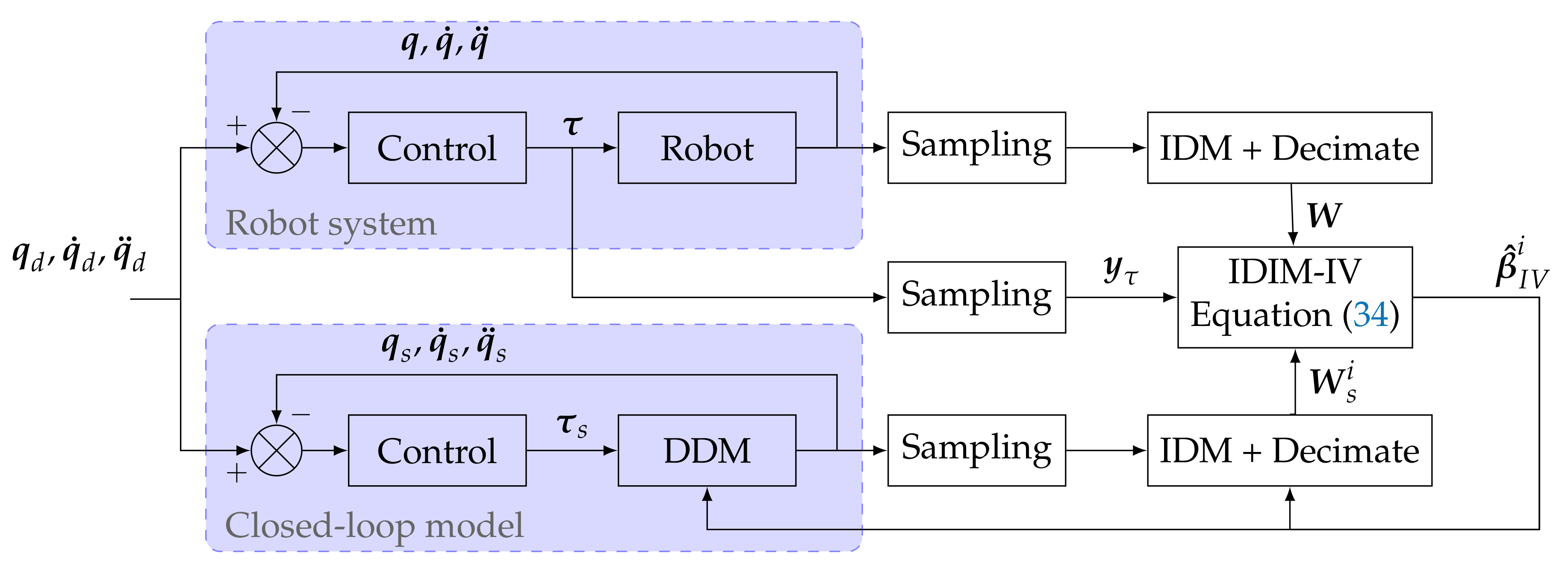
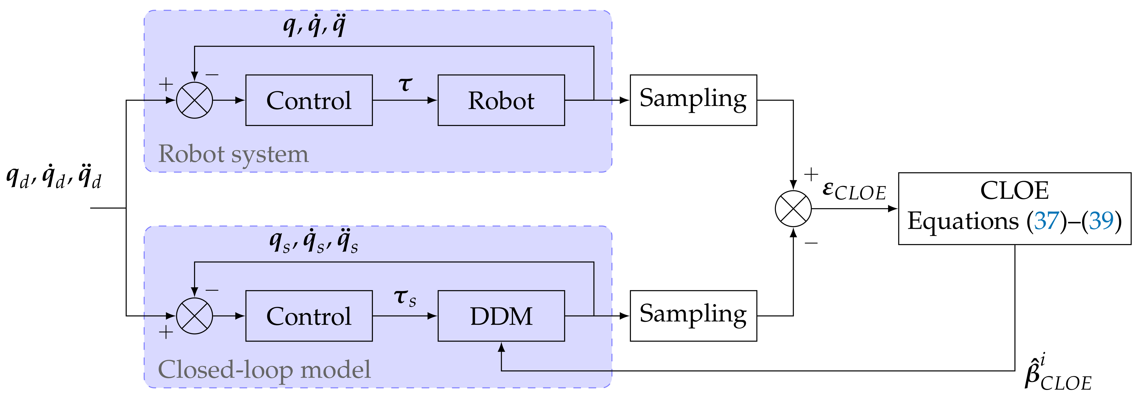
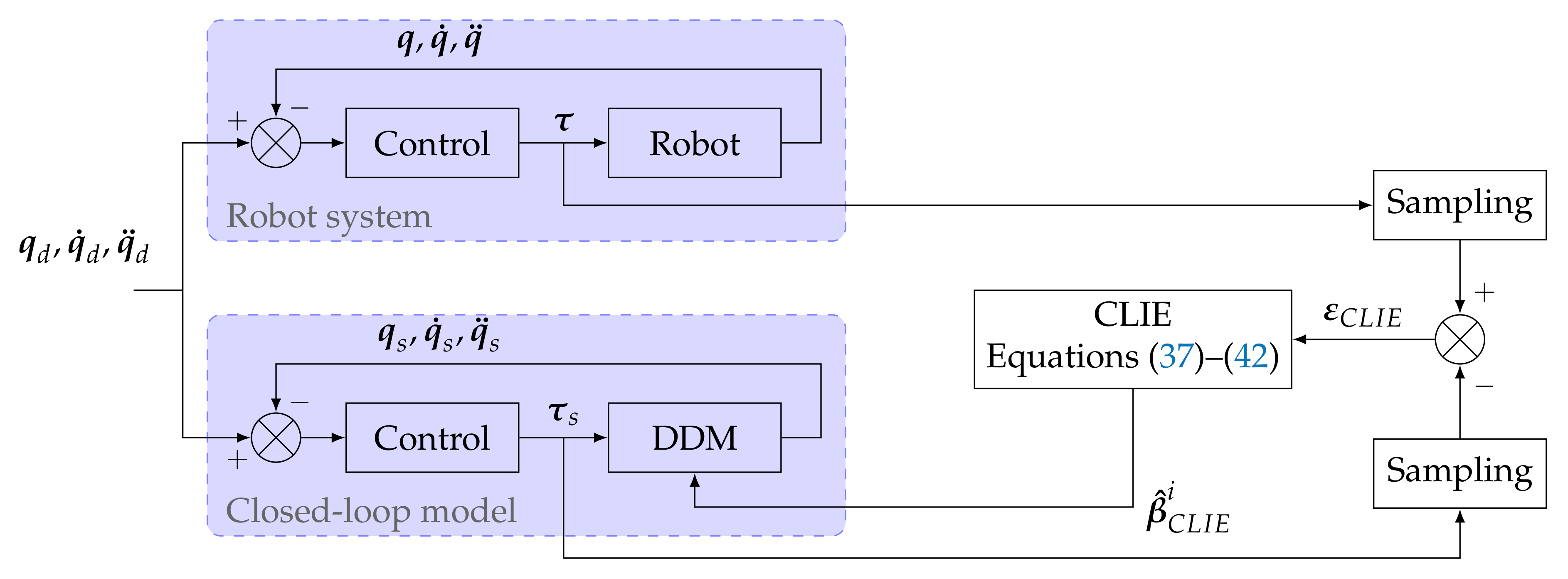
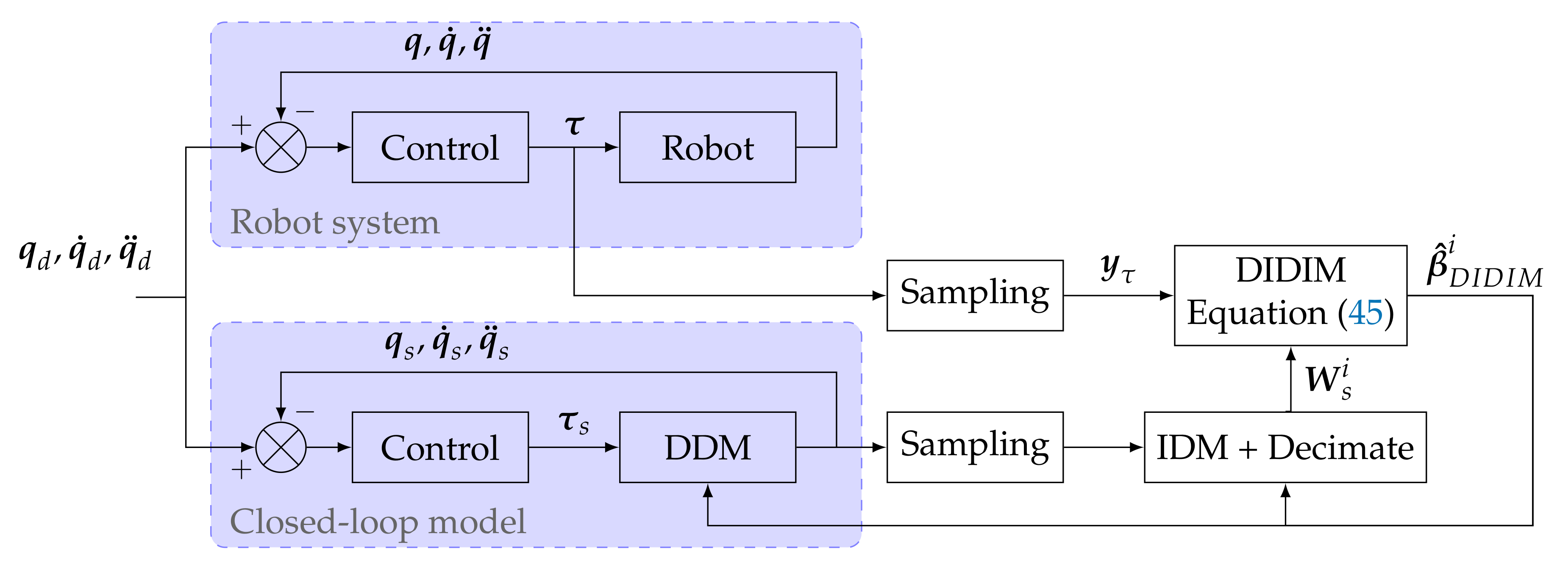
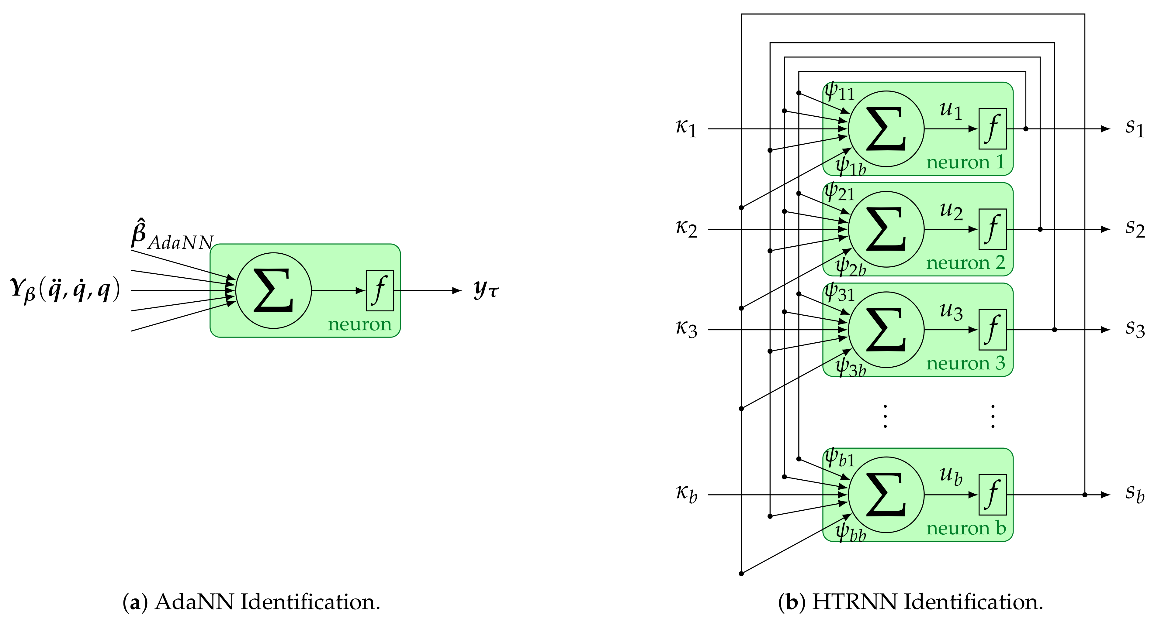
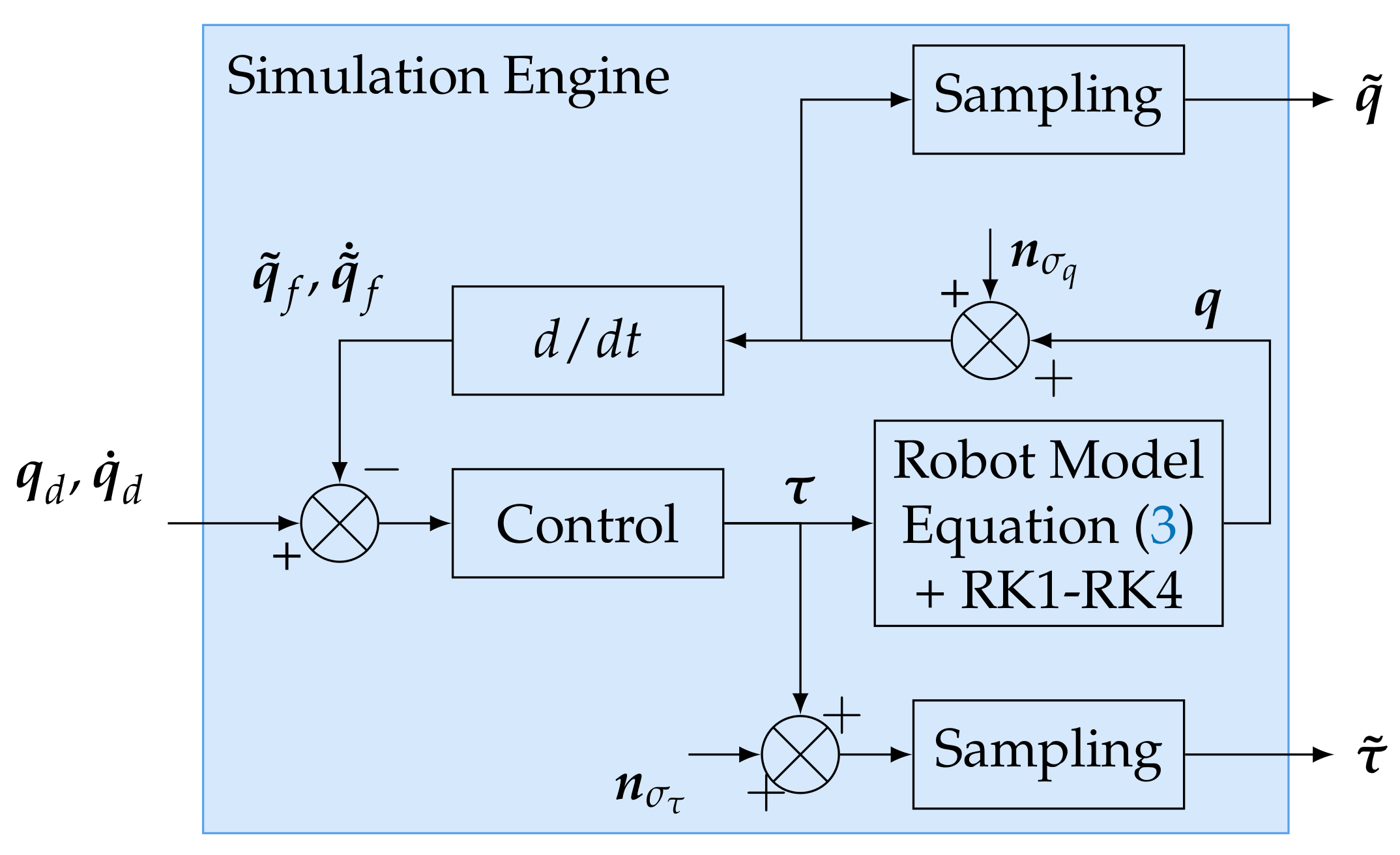
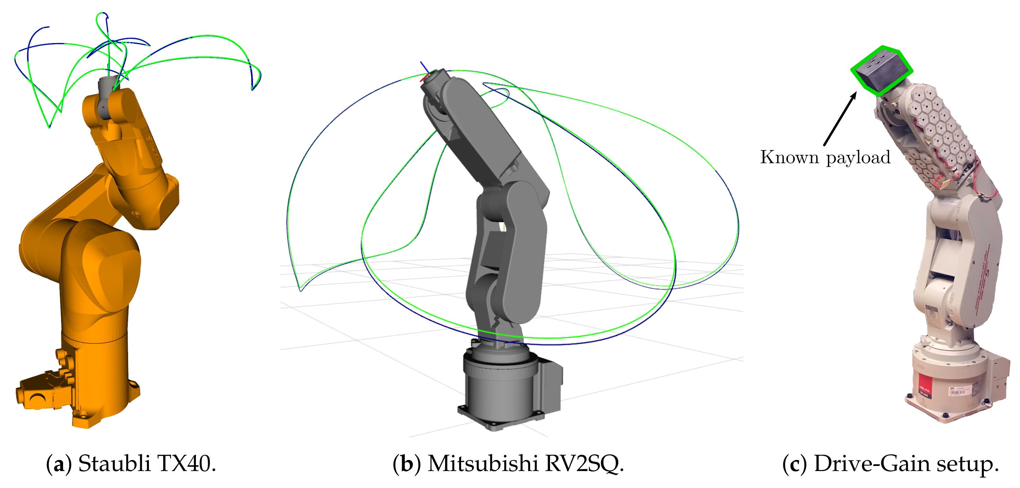
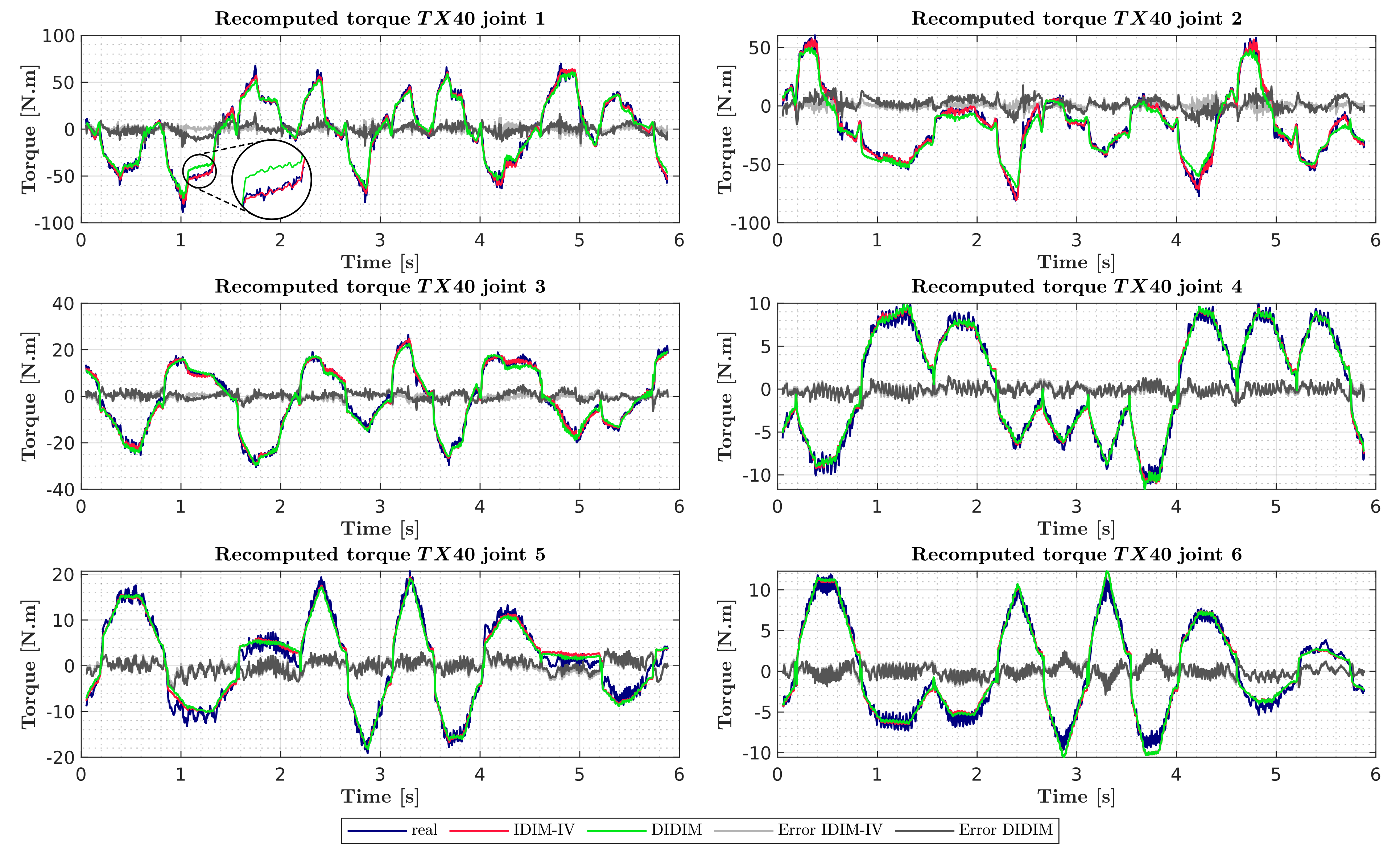
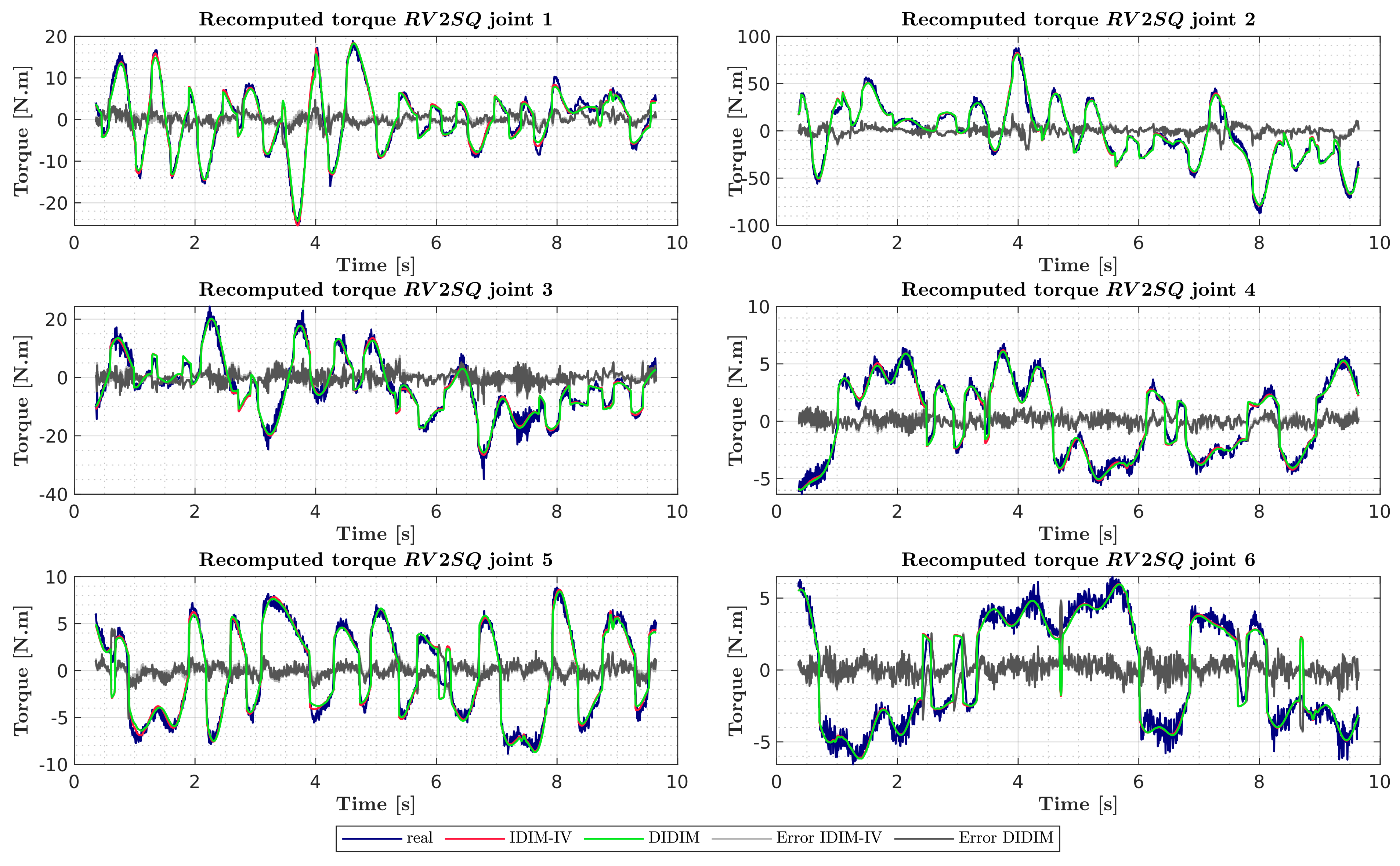
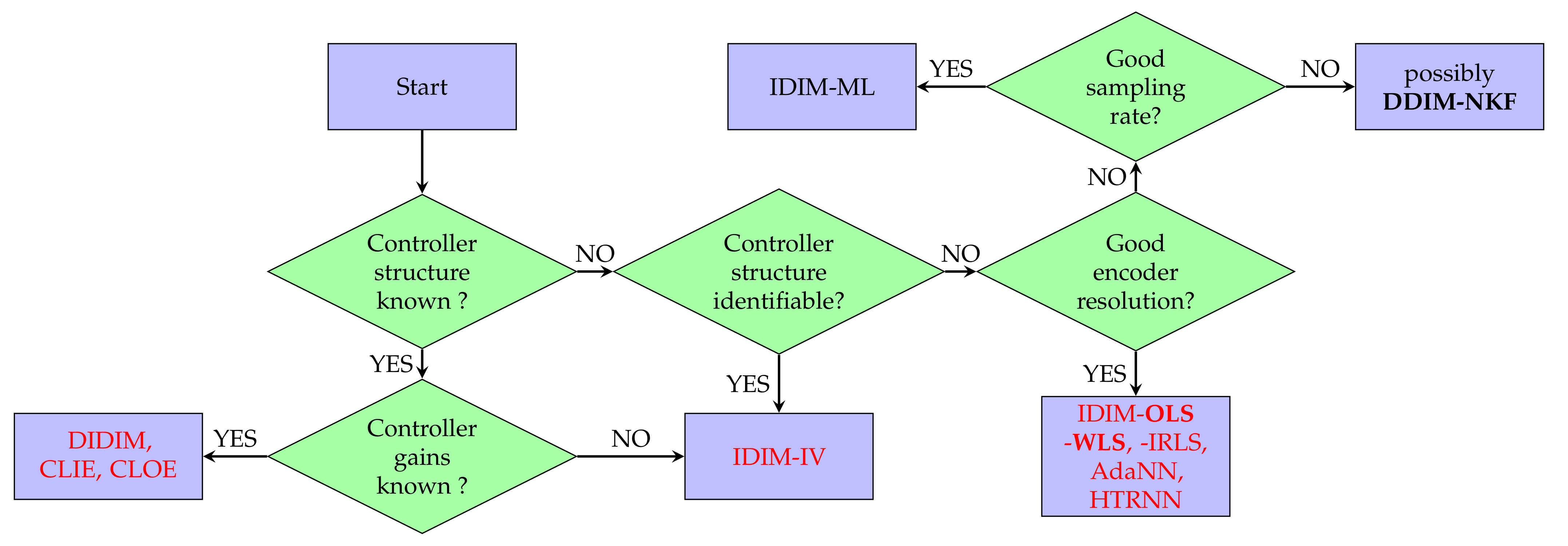
Table A1.
Overview of the different identification methods implemented in this work.
| Least-Squares | OLS, WLS, TLS, IRLS |
| Output Error | CLIE, CLOE, DIDIM |
| Kalman Filters | EKF, SREKF, UKF, SRUKF, CDKF, SRCDKF |
| Neural Networks | AdaNN, HTRNN |
| Other | IDIM-IV, ML |
| Physically Consistent | PC-OLS, PC-WLS, PC-IRLS, PC-IV, PC-DIDIM |
References
- Lee, T.; Kwon, J.; Park, F.C. A natural adaptive control law for robot manipulators. In Proceedings of the 2018 IEEE/RSJ International Conference on Intelligent Robots and Systems (IROS), Madrid, Spain, 1–5 October 2018; pp. 1–9. [Google Scholar]
- Gautier, M. Dynamic identification of robots with power model. In Proceedings of the 1997 IEEE International Conference on Robotics and Automation, Albuquerque, NX, USA, 20–25 April 1997; Volume 3, pp. 1922–1927. [Google Scholar]
- Siciliano, B.; Khatib, O. Springer Handbook of Robotics; Springer: Berlin, Germany, 2016. [Google Scholar]
- Van Huffel, S.; Vandewalle, J. The Total Least Squares Problem: Computational Aspects and Analysis; Siam; Society for Industrial and Applied Mathematics: Philadelphia, PA, USA, 1991; Volume 9. [Google Scholar] [CrossRef]
- Janot, A.; Gautier, M.; Jubien, A.; Vandanjon, P.O. Comparison between the CLOE Method and the DIDIM Method for Robots Identification. IEEE Trans. Control Syst. Technol. 2014, 22, 1935–1941. [Google Scholar]
- Janot, A.; Vandanjon, P.O.; Gautier, M. A generic instrumental variable approach for industrial robot identification. IEEE Trans. Control Syst. Technol. 2014, 22, 132–145. [Google Scholar]
- Gautier, M.; Poignet, P. Extended Kalman filtering and weighted least squares dynamic identification of robot. Control Eng. Pract. 2001, 9, 1361–1372. [Google Scholar]
- Ramdani, N.; Poignet, P. Robust dynamic experimental identification of robots with set membership uncertainty. IEEE/ASME Trans. Mechatron. 2005, 10, 253–256. [Google Scholar]
- Swevers, J.; Ganseman, C.; Tukel, D.B.; De Schutter, J.; Van Brussel, H. Optimal robot excitation and identification. IEEE Trans. Robot. Autom. 1997, 13, 730–740. [Google Scholar]
- Olsen, M.M.; Petersen, H.G. A new method for estimating parameters of a dynamic robot model. IEEE Trans. Robot. Autom. 2001, 17, 95–100. [Google Scholar]
- Olsen, M.M.; Swevers, J.; Verdonck, W. Maximum Likelihood Identification of a Dynamic Robot Model: Implementation Issues. Int. J. Robot. Res. 2002, 21, 89–96. [Google Scholar] [CrossRef]
- Brunot, M.; Janot, A.; Carrillo, F.; Cheong, J.; Jean-Philippe, N. Output error methods for robot identification. IEEE/ASME Trans. Mechatron. 2019. [Google Scholar] [CrossRef] [Green Version]
- Urrea, C.; Pascal, J. Design, simulation, comparison and evaluation of parameter identification methods for an industrial robot. Comput. Electr. Eng. 2016, 67, 791–806. [Google Scholar] [CrossRef]
- Urrea, C.; Pascal, J. Parameter identification methods for real redundant manipulators. J. Appl. Res. Technol. 2017, 15, 320–331. [Google Scholar]
- Yoshida, K.; Khalil, W. Verification of the positive definiteness of the inertial matrix of manipulators using base inertial parameters. Int. J. Robot. Res. 2000, 19, 498–510. [Google Scholar]
- Mata, V.; Benimeli, F.; Farhat, N.; Valera, A. Dynamic parameter identification in industrial robots considering physical feasibility. Adv. Robot. 2005, 19, 101–119. [Google Scholar]
- Jovic, J.; Philipp, F.; Escande, A.; Ayusawa, K.; Yoshida, E.; Kheddar, A.; Venture, G. Identification of dynamics of humanoids: Systematic exciting motion generation. In Proceedings of the 2015 IEEE/RSJ International Conference on Intelligent Robots and Systems (IROS), Hamburg, Germany, 28 September–2 October 2015; pp. 2173–2179. [Google Scholar]
- Gaz, C.; Flacco, F.; De Luca, A. Extracting feasible robot parameters from dynamic coefficients using nonlinear optimization methods. In Proceedings of the 2016 IEEE International Conference on Robotics and Automation (ICRA), Stockholm, Sweden, 16–21 May 2016; pp. 2075–2081. [Google Scholar]
- Sutanto, G.; Wang, A.; Lin, Y.; Mukadam, M.; Sukhatme, G.; Rai, A.; Meier, F. Encoding physical constraints in differentiable newton-euler algorithm. arXiv 2020, arXiv:2001.08861. [Google Scholar]
- Sousa, C.D.; Cortesão, R. Physical feasibility of robot base inertial parameter identification: A linear matrix inequality approach. Int. J. Robot. Res. 2014, 33, 931–944. [Google Scholar]
- Sousa, C.D.; Cortesão, R. Inertia Tensor Properties in Robot Dynamics Identification: A Linear Matrix Inequality Approach. IEEE/ASME Trans. Mechatronics 2019, 24, 406–411. [Google Scholar] [CrossRef]
- Wensing, P.M.; Kim, S.; Slotine, J.J.E. Linear Matrix Inequalities for Physically Consistent Inertial Parameter Identification: A Statistical Perspective on the Mass Distribution. IEEE Robot. Autom. Lett. 2018, 3, 60–67. [Google Scholar] [CrossRef]
- Han, Y.; Wu, J.; Liu, C.; Xiong, Z. An Iterative Approach for Accurate Dynamic Model Identification of Industrial Robots. IEEE Trans. Robot. 2020, 36, 1577–1594. [Google Scholar]
- Traversaro, S.; Brossette, S.; Escande, A.; Nori, F. Identification of fully physical consistent inertial parameters using optimization on manifolds. In Proceedings of the 2016 IEEE/RSJ International Conference on Intelligent Robots and Systems (IROS), Daejeon, Korea, 9–14 October 2016; pp. 5446–5451. [Google Scholar]
- Lee, T.; Park, F.C. A geometric algorithm for robust multibody inertial parameter identification. IEEE Robot. Autom. Lett. 2018, 3, 2455–2462. [Google Scholar]
- Lee, T.; Wensing, P.M.; Park, F.C. Geometric robot dynamic identification: A convex programming approach. IEEE Trans. Robot. 2019, 36, 348–365. [Google Scholar]
- Bargsten, V.; de Gea Fernandez, J.; Kassahun, Y. Experimental robot inverse dynamics identification using classical and machine learning techniques. Proceedings of ISR 2016: 47st International Symposium on Robotics, VDE, Munich, Germany, 21–26 June 2016; pp. 1–6. [Google Scholar]
- Ledezma, F.D.; Haddadin, S. First-order-principles-based constructive network topologies: An application to robot inverse dynamics. In Proceedings of the 2017 IEEE-RAS 17th International Conference on Humanoid Robotics (Humanoids), Birmingham, UK, 15–17 November 2017; pp. 438–445. [Google Scholar]
- Wu, J.; Wang, J.; You, Z. An overview of dynamic parameter identification of robots. Robot. Comput. Integr. Manuf. 2010, 26, 414–419. [Google Scholar]
- Hjalmarsson, H.; Rojas, C.R.; Rivera, D.E. System identification: A Wiener-Hammerstein benchmark. Control Eng. Pract. 2012, 20, 1095–1096. [Google Scholar] [CrossRef]
- Kroll, A.; Schulte, H. Benchmark problems for nonlinear system identification and control using soft computing methods: Need and overview. Appl. Soft Comput. 2014, 25, 496–513. [Google Scholar] [CrossRef]
- Rojas, C.R.; Valenzuela, P.E.; Rojas, R.A. A critical view on benchmarks based on randomly generated systems. In Proceedings of the 17th IFAC Symposium on System Identification (IFAC, 2015), Beijing, China, 19–21 October 2015. [Google Scholar]
- Bethge, S.; Malzahn, J.; Tsagarakis, N.; Caldwell, D. FloBaRoID—A software package for the identification of robot dynamics parameters. In Proceedings of the International Conference on Robotics in Alpe-Adria Danube Region, Futuroscope-Poitiers, France, 21–23 June 2017; Springer: Berlin, Germany, 2017; pp. 156–165. [Google Scholar]
- Wang, Y.; Gondokaryono, R.; Munawar, A.; Fischer, G.S. A convex optimization-based dynamic model identification package for the da Vinci Research Kit. IEEE Robot. Autom. Lett. 2019, 4, 3657–3664. [Google Scholar]
- Chaicherdkiat, P.; Osterloh, T.; Netramai, C.; Reßmann, J. Simulation-based Parameter Identification Framework for the Calibration of Rigid Body Simulation Models. In Proceedings of the IEEE 2020 SICE International Symposium on Control Systems (SICE ISCS), Tokushima, Japan, 3–5 March 2020; pp. 12–19. [Google Scholar]
- Spong, M.W.; Vidyasagar, M. Robot Dynamics And Control; John Wiley & Sons: Hoboken, NJ, USA, 2008. [Google Scholar]
- Khalil, W.; Dombre, E. Modeling, Identification and Control of Robots; Butterworth-Heinemann: Oxford, UK, 2004. [Google Scholar]
- Gautier, M.; Khalil, W. Exciting trajectories for the identification of base inertial parameters of robots. Int. J. Robot. Res. 1992, 11, 362–375. [Google Scholar]
- Gautier, M.; Khalil, W. Direct calculation of minimum set of inertial parameters of serial robots. IEEE Trans. Robot. Autom. 1990, 6, 368–373. [Google Scholar]
- Mayeda, H.; Yoshida, K.; Osuka, K. Base parameters of manipulator dynamic models. IEEE Trans. Robot. Autom. 1990, 6, 312–321. [Google Scholar]
- Beschi, M.; Villagrossi, E.; Pedrocchi, N.; Tosatti, L.M. A general analytical procedure for robot dynamic model reduction. In Proceedings of the 2015 IEEE/RSJ International Conference on Intelligent Robots and Systems (IROS), Hamburg, Germany, 28 September–2 October 2015; pp. 4127–4132. [Google Scholar]
- Gautier, M.; Briot, S.; Venture, G. Identification of consistent standard dynamic parameters of industrial robots. In Proceedings of the 2013 IEEE/ASME International Conference on Advanced Intelligent Mechatronics, Wollongong, Australia, 9–12 July 2013; pp. 1429–1435. [Google Scholar]
- Gautier, M.; Janot, A.; Vandanjon, P.O. A new closed-loop output error method for parameter identification of robot dynamics. IEEE Trans. Control Syst. Technol. 2013, 21, 428–444. [Google Scholar]
- Jubien, A.; Gautier, M.; Janot, A. Dynamic identification of the Kuka LWR robot using motor torques and joint torque sensors data. IFAC Proc. Vol. 2014, 47, 8391–8396. [Google Scholar]
- Venture, G.; Ripert, P.; Khalil, W.; Gautier, M.; Bodson, P. Modeling and Identification of Passenger Car Dynamics Using Robotics Formalism. IEEE Trans. Intell. Transp. Syst. 2006, 7, 349–359. [Google Scholar] [CrossRef]
- Khatounian, F.; Moreau, S.; Monmasson, E.; Janot, A.; Louveau, F. Parameters Estimation of the Actuator used in Haptic Interfaces: Comparison of two Identification Methods. In Proceedings of the 2006 IEEE International Symposium on Industrial Electronics, Montreal, QC, Canada, 9–13 July 2006; Volume 1, pp. 211–216. [Google Scholar] [CrossRef]
- Lemaire, C.E.; Vandanjon, P.O.; Gautier, M.; Lemaire, C. Dynamic Identification of a Vibratory Asphalt Compactor for Contact Efforts Estimation. In Proceedings of the 14th IFAC Symposium on Identification and System Parameter Estimation, Newcastle, Australia, 29–31 March 2006; Volume 39, pp. 973–978. [Google Scholar] [CrossRef]
- Huber, P.J. The 1972 wald lecture robust statistics: A review. Ann. Math. Stat. 1972, 43, 1041–1067. [Google Scholar]
- Huber, P.J. Robust regression: Asymptotics, conjectures and Monte Carlo. Ann. Math. Stat. 1973, 1, 799–821. [Google Scholar]
- Holland, P.W.; Welsch, R.E. Robust regression using iteratively reweighted least-squares. Commun. Stat. Theory Methods 1977, 6, 813–827. [Google Scholar]
- Janot, A.; Vandanjon, P.O.; Gautier, M. Using robust regressions and residual analysis to verify the reliability of LS estimation: Application in robotics. In Proceedings of the 2009 IEEE/RSJ International Conference on Intelligent Robots and Systems, St. Louis, MI, USA, 11–15 October 2009; pp. 1962–1967. [Google Scholar]
- Brunot, M.; Janot, A.; Young, P.C.; Carrillo, F. An improved instrumental variable method for industrial robot model identification. Control Eng. Pract. 2018, 74, 107–117. [Google Scholar]
- Swevers, J.; Verdonck, W.; De Schutter, J. Dynamic model identification for industrial robots. IEEE Control Syst. 2007, 27, 58–71. [Google Scholar]
- Xi, F. Effect of non-geometric errors on manipulator inertial calibration. Proceedings of 1995 IEEE International Conference on Robotics and Automation, Nagoya, Japan, 21–27 May 1995; Volume 2, pp. 1808–1813. [Google Scholar] [CrossRef]
- Bjorck, A. Numerical Methods for Least Squares Problems; Siam: Philadelphia, PA, USA, 1996; Volume 51. [Google Scholar] [CrossRef]
- Rhode, S.; Usevich, K.; Markovsky, I.; Gauterin, F. A recursive restricted total least-squares algorithm. IEEE Trans. Signal Process. 2014, 62, 5652–5662. [Google Scholar]
- Van Huffel, S.; Vandewalle, J. Comparison of total least squares and instrumental variable methods for parameter estimation of transfer function models. Int. J. Control 1989, 50, 1039–1056. [Google Scholar]
- Söderström, T.; Mahata, K. On instrumental variable and total least squares approaches for identification of noisy systems. Int. J. Control 2002, 75, 381–389. [Google Scholar]
- Janot, A. On the Identification of Continuous-Time Inverse Dynamic Model of Electromechanical Systems Operating in Closed Loop with an Instrumental Variable Approach: Application to Industrial Robots. Ph.D. Thesis, Centre Midi Pyrenees Toulouse, Toulouse, France, 2017. [Google Scholar]
- Janot, A.; Vandanjon, P.O.; Gautier, M. A revised Durbin-Wu-Hausman test for industrial robot identification. Control Eng. Pract. 2016, 48, 52–62. [Google Scholar]
- Van Huffel, S.; Vandewalle, J. Analysis and properties of the generalized total least squares problem AX=B when some or all columns in A are subject to error. SIAM J. Matrix Anal. Appl. 1989, 10, 294–315. [Google Scholar]
- Gautier, M.; Briot, S. Global Identification of Joint Drive Gains and Dynamic Parameters of Robots. J. Dyn. Syst. Meas. Control 2014, 136, 1–9. [Google Scholar]
- Markovsky, I.; Huffel, S.V. Overview of total least-squares methods. Signal Process. 2007, 87, 2283–2302. [Google Scholar] [CrossRef] [Green Version]
- Reiersøl, O. Confluence analysis by means of lag moments and other methods of confluence analysis. Econ. J. Econ. Soc. 1941, 1–24. [Google Scholar]
- Söderström, T.; Stoica, P. Instrumental variable methods for system identification. Circ. Syst. Signal Process. 2002, 21, 1–9. [Google Scholar]
- Young, P. Recursive Estimation and Time-Series Analysis: An Introduction for the Student and Practitioner; Springer: Berlin, Germany, 2011. [Google Scholar]
- Puthenpura, S.C.; Sinha, N.K. Identification of continuous-time systems using instrumental variables with application to an industrial robot. IEEE Trans. Ind. Electr. 1986, 224–229. [Google Scholar]
- Yoshida, K.; Ikeda, N.; Mayeda, H. Experimental study of the identification methods for an industrial robot manipulator. In Proceedings of the 1992 lEEE/RSJ International Conference on Intelligent Robots and Systems, Raleigh, NC, USA, 7–10 July 1992; Volume 1, pp. 263–270. [Google Scholar]
- Brunot, M. Identification of Rigid Industrial Robots—A System Identification Perspective. Ph.D. Thesis, INPT, Toulouse, France, 2017. [Google Scholar]
- Brunot, M.; Janot, A.; Carrillo, F. An automated instrumental variable method for rigid industrial robot identification. IFAC-PapersOnLine 2018, 51, 431–436. [Google Scholar]
- Young, P.C. Refined instrumental variable estimation: Maximum likelihood optimization of a unified Box–Jenkins model. Automatica 2014, 52, 35–46. [Google Scholar]
- Landau, I.D.; Karimi, A. An output error recursive algorithm for unbiased identification in closed loop. Automatica 1997, 33, 933–938. [Google Scholar]
- Landau, I.; Anderson, B.; De Bruyne, F. Closed-loop output error identification algorithms for nonlinear plants. In Proceedings of the 1999 38th IEEE Conference on Decision and Control, Phoenix, AZ, USA, 7–10 December 1999; Volume 1, pp. 606–611. [Google Scholar]
- Aivaliotis, P.; Papalitsa, E.; Michalos, G.; Makris, S. Identification of dynamic robot’s parameters using physics-based simulation models for improving accuracy. Procedia CIRP 2021, 96, 254–259. [Google Scholar]
- Gautier, M.; Vandanjon, P.O.; Janot, A. Dynamic identification of a 6 dof robot without joint position data. In Proceedings of the 2011 IEEE International Conference on Robotics and Automation, Shanghai, China, 9–13 May 2011; pp. 234–239. [Google Scholar]
- Brunot, M.; Janot, A.; Carrillo, F.; Garnier, H. Comparison between the IDIM-IV method and the DIDIM method for industrial robots identification. In Proceedings of the 2017 IEEE International Conference on Advanced Intelligent Mechatronics (AIM), Munich, Germany, 3–7 July 2017; pp. 571–576. [Google Scholar] [CrossRef] [Green Version]
- Wan, E.A.; Van Der Merwe, R.; Nelson, A.T. Dual estimation and the unscented transformation. In Advances in Neural Information Processing Systems; MIT Press: Denver, CO, USA, 27–30 November 2000; pp. 666–672. [Google Scholar]
- Paul, A.S.; Wan, E.A. Dual Kalman filters for autonomous terrain aided navigation in unknown environments. In Proceedings of the 2005 IEEE International Joint Conference on Neural Networks, IJCNN’05, Montreal, QC, Canada, 31 July–4 August 2005; Volume 5, pp. 2784–2789. [Google Scholar]
- Joukov, V.; Bonnet, V.; Venture, G.; Kulić, D. Constrained dynamic parameter estimation using the extended Kalman filter. In Proceedings of the 2015 IEEE/RSJ International Conference on Intelligent Robots and Systems (IROS), Hamburg, Germany, 28 September–2 October 2015; pp. 3654–3659. [Google Scholar]
- Dellon, B.; Matsuoka, Y. Modeling and system identification of a life-size brake-actuated manipulator. IEEE Trans. Robot. 2009, 25, 481–491. [Google Scholar]
- Riva, M.H.; Wielitzka, M.; Ortmaier, T. Sensitivity-Based Adaptive SRUKF for State, Parameter, and Covariance Estimation on Mechatronic Systems. In Kalman Filters: Theory for Advanced Applications; Intech Open: Rijeka, Croatia, 2018; p. 77. [Google Scholar] [CrossRef]
- Van Der Merwe, R. Sigma-Point Kalman Filters for Probabilistic Inference in Dynamic State-Space Models. PhD Thesis, OGI School of Science & Engineering at Oregon Health & Science University, Portland, OR, USA, 2004. [Google Scholar]
- Featherstone, R. Rigid Body Dynamics Algorithms; Springer: Berlin, Germany, 2014. [Google Scholar]
- Liu, J.; West, M. Combined parameter and state estimation in simulation-based filtering. In Sequential Monte Carlo Methods in Practice; Springer: Berlin, Germany, 2001; pp. 197–223. [Google Scholar]
- Arulampalam, M.S.; Maskell, S.; Gordon, N.; Clapp, T. A tutorial on particle filters for online nonlinear/non-Gaussian Bayesian tracking. IEEE Trans. Signal Process. 2002, 50, 174–188. [Google Scholar]
- Bottou, L. Stochastic gradient descent tricks. In Neural Networks: Tricks of the Trade; Springer: Berlin, Germany, 2012; pp. 421–436. [Google Scholar]
- Hopfield, J.J.; Tank, D.W. “Neural” computation of decisions in optimization problems. Biol. Cybern. 1985, 52, 141–152. [Google Scholar]
- Atencia, M.; Joya, G.; Sandoval, F. Hopfield neural networks for parametric identification of dynamical systems. Neural Process. Lett. 2005, 21, 143–152. [Google Scholar]
- Abe, S. Theories on the Hopfield neural networks. In Proceedings of the International 1989 Joint Conference on Neural Networks, Washington, DC, USA, 18–21 June 1989; Volume 1, pp. 557–564. [Google Scholar] [CrossRef]
- Smith, K.; Palaniswami, M.; Krishnamoorthy, M. Neural techniques for combinatorial optimization with applications. IEEE Trans. Neural Netw. 1998, 9, 1301–1318. [Google Scholar]
- Hopfield, J.J. Neurons with graded response have collective computational properties like those of two-state neurons. Proc. Natl. Acad. Sci. USA 1984, 81, 3088–3092. [Google Scholar]
- Janot, A.; Wensing, P.M. Sequential semidefinite optimization for physically and statistically consistent robot identification. Control Eng. Pract. 2021, 107, 104699. [Google Scholar] [CrossRef]
- Ayusawa, K.; Nakamura, Y. Identification of standard inertial parameters for large-dof robots considering physical consistency. In Proceedings of the 2010 IEEE/RSJ International Conference on Intelligent Robots and Systems, Taipei, Taiwan, 18–22 October 2010; pp. 6194–6201. [Google Scholar]
- Gautier, M.; Venture, G. Identification of standard dynamic parameters of robots with positive definite inertia matrix. In Proceedings of the 2013 IEEE/RSJ International Conference on Intelligent Robots and Systems, Tokyo, Japan, 3–7 November 2013; pp. 5815–5820. [Google Scholar]
- Antonelli, G.; Caccavale, F.; Chiacchio, P. A systematic procedure for the identification of dynamic parameters of robot manipulators. Robotica 1999, 17, 427–435. [Google Scholar]
- Corke, P.I. A robotics toolbox for MATLAB. IEEE Robot. Autom. Mag. 1996, 3, 24–32. [Google Scholar]
- Sciavicco, L.; Siciliano, B.; Villani, L. Lagrange and Newton-Euler dynamic modeling of a gear-driven robot manipulator with inclusion of motor inertia effects. Adv. Robot. 1995, 10, 317–334. [Google Scholar]
- Jung, D.; Cheong, J.; Park, D.I.; Park, C. Backward sequential approach for dynamic parameter identification of robot manipulators. Int. J. Adv. Robot. Syst. 2018, 15, 1729881418758578. [Google Scholar]
- Calafiore, G.; Indri, M.; Bona, B. Robot dynamic calibration: Optimal excitation trajectories and experimental parameter estimation. J. Robot. Syst. 2001, 18, 55–68. [Google Scholar]
- Jin, J.; Gans, N. Parameter identification for industrial robots with a fast and robust trajectory design approach. Robot. Comput. Integr. Manuf. 2015, 31, 21–29. [Google Scholar]
- Abu-Dakka, F.J.; Díaz-Rodríguez, M. Comparison of trajectory parametrization methods with statistical analysis for dynamic parameter identification of serial robot. In Proceedings of the 2017 IEEE/RSJ International Conference on Intelligent Robots and Systems (IROS), Vancouver, BC, Canada, 24–28 September 2017; pp. 5874–5879. [Google Scholar]
- Ayusawa, K.; Rioux, A.; Yoshida, E.; Venture, G.; Gautier, M. Generating persistently exciting trajectory based on condition number optimization. In Proceedings of the 2017 IEEE International Conference on Robotics and Automation (ICRA), Singapore, 29 May–3 June 2017; pp. 6518–6524. [Google Scholar]
- De Wit, C.C.; Olsson, H.; Astrom, K.J.; Lischinsky, P. A new model for control of systems with friction. IEEE Trans. Autom. Control 1995, 40, 419–425. [Google Scholar]
- Gautier, M.; Briot, S. New method for global identification of the joint drive gains of robots using a known payload mass. In Proceedings of the 2011 IEEE/RSJ International Conference on Intelligent Robots and Systems, San Francisco, CA, USA, 25–30 September 2011; pp. 3728–3733. [Google Scholar]
- Gautier, M.; Briot, S. Global identification of drive gains parameters of robots using a known payload. In Proceedings of the 2012 IEEE International Conference on Robotics and Automation, Saint Paul, MN, USA, 14–18 May 2012; pp. 2812–2817. [Google Scholar]
- Hashemi, S.M.; Werner, H. Parameter identification of a robot arm using separable least squares technique. In Proceedings of the 2009 European Control Conference (ECC), Budapest, Hungary, 23–26 August 2009; pp. 2199–2204. [Google Scholar]
- Bona, B.; Indri, M. Friction compensation in robotics: An overview. In Proceedings of the 44th IEEE Conference on Decision and Control, Seville, Spain, 12–15 December 2005; pp. 4360–4367. [Google Scholar] [CrossRef]
- Atencia, M.; Joya, G.; Sandoval, F. Parametric identification of robotic systems with stable time-varying Hopfield networks. Neural Comput. Appl. 2004, 13, 270–280. [Google Scholar]
- Grant, M.; Boyd, S. CVX: Matlab Software for Disciplined Convex Programming, version 2.1; 2014. Available online: http://cvxr.com/ (accessed on 8 May 2020).
- MOSEK Optimization Suite. 2019. Available online: https://www.mosek.com/ (accessed on 8 May 2020).
- Suter, B.W. Multirate and Wavelet Signal Processing; Elsevier: Amsterdam, The Netherlands, 1997. [Google Scholar]
- Khalil, W.; Creusot, D. SYMORO+: A system for the symbolic modelling of robots. Robotica 1997, 15, 153–161. [Google Scholar]
- Khalil, W.; Vijayalingam, A.; Khomutenko, B.; Mukhanov, I.; Lemoine, P.; Ecorchard, G. OpenSYMORO: An open-source software package for Symbolic Modelling of Robots. In Proceedings of the 2014 IEEE/ASME International Conference on Advanced Intelligent Mechatronics, Besancon, France, 8–11 July 2014; pp. 1206–1211. [Google Scholar]
- Felis, M.L. RBDL: An efficient rigid-body dynamics library using recursive algorithms. Auton. Robot. 2017, 41, 495–511. [Google Scholar]
- Smits, R.; Bruyninckx, H.; Aertbeliën, E. KDL: Kinematics and Dynamics Library. 2011. Available online: https://github.com/rbdl/rbdl (accessed on 8 May 2020).
- Iwasaki, T.; Venture, G.; Yoshida, E. Identification of the inertial parameters of a humanoid robot using grounded sole link. In Proceedings of the 2012 12th IEEE-RAS International Conference on Humanoid Robots (Humanoids 2012), Osaka, Japan, 29 November–1 December 2012; pp. 449–454. [Google Scholar]
- Jovic, J.; Escande, A.; Ayusawa, K.; Yoshida, E.; Kheddar, A.; Venture, G. Humanoid and human inertia parameter identification using hierarchical optimization. IEEE Trans. Robot. 2016, 32, 726–735. [Google Scholar]
Figure 1.
Block diagram of the IDIM-IV identification method.

Figure 2.
Block diagram of the CLOE identification method.

Figure 3.
Block diagram of the Closed-Loop Input Error (CLIE) identification method.

Figure 4.
Block diagram of the DIDIM identification method.

Figure 5.
Adaline and Hopfield Neural Networks used for Inertial Parameter Identification.

Figure 6.
Block diagram of BIRDy, the Benchmark for Identification of Robot Dynamics. In this figure, refers to the desired trajectory data, obtained from the trajectory interpolator, respectively denote the noisy joint positions, torques and (in the case of a real robot) drive current measurements. The actual data used for identification, is obtained after a short pre-processing step of the raw experiment data.

Figure 7.
Detail of the “Simulation Engine” of Figure 6.
Figure 7.
Detail of the “Simulation Engine” of Figure 6.

Figure 8.
The left and center figures denote the end-effector trajectories—desired in green and actual in dark blue—executed during the experiments on the real robots and visualized on Rviz using the Matlab-ROS interface. The excitation trajectory of the TX40 was manually generated, with trapezoidal velocity profiles and was later imported into BIRDy, while that of the RV2SQ was directly generated using the benchmark Fourier trajectory generation tool. The rightmost figure depicts the experiment setup used for drive gains identification on the Mitsubishi RV2SQ. Note the external payload, with known inertial parameters, attached to the end-effector of the robot.

Figure 9.
Reconstructed IDIM-IV and DIDIM torque signals during the validation experiment on the real TX40 robot.
Figure 9.
Reconstructed IDIM-IV and DIDIM torque signals during the validation experiment on the real TX40 robot.

Figure 10.
Reconstructed IDIM-IV and DIDIM torque signals during the validation experiment on the real RV2SQ robot.
Figure 10.
Reconstructed IDIM-IV and DIDIM torque signals during the validation experiment on the real RV2SQ robot.

Figure 11.
Decision process for parameter identification algorithm selection. Physical consistency of the estimates can be enforced using SDP within the algorithms displayed in red. Methods in bold caption are, or can potentially be formulated in a recursive manner which makes them capable of running in a real-time control loop.

Table 1.
Overview and naming convention of the different experiments performed during the MCS. The first row of the table refers to noise conditions that are close to what can be encountered on an industrial robot manipulator. The four other rows explore the performance of identification in the case of substantially higher joint position and torque noise levels.
| MCS Experimental Conditions | TX40 Decimation 1 | TX40 Decimation 4 | RV2SQ Decimation 1 |
|---|---|---|---|
| MCS-TX40-1-1 | MCS-TX40-4-1 | MCS-RV2SQ-1-1 | |
| MCS-TX40-1-2 | MCS-TX40-4-2 | MCS-RV2SQ-1-2 | |
| MCS-TX40-1-3 | MCS-TX40-4-3 | MCS-RV2SQ-1-3 | |
| MCS-TX40-1-4 | MCS-TX40-4-4 | MCS-RV2SQ-1-4 | |
| MCS-TX40-1-5 | MCS-TX40-4-5 | MCS-RV2SQ-1-5 |
Publisher’s Note: MDPI stays neutral with regard to jurisdictional claims in published maps and institutional affiliations. |
© 2021 by the authors. Licensee MDPI, Basel, Switzerland. This article is an open access article distributed under the terms and conditions of the Creative Commons Attribution (CC BY) license (https://creativecommons.org/licenses/by/4.0/).
Share and Cite
MDPI and ACS Style
Leboutet, Q.; Roux, J.; Janot, A.; Guadarrama-Olvera, J.R.; Cheng, G. Inertial Parameter Identification in Robotics: A Survey. Appl. Sci. 2021, 11, 4303. https://0-doi-org.brum.beds.ac.uk/10.3390/app11094303
AMA Style
Leboutet Q, Roux J, Janot A, Guadarrama-Olvera JR, Cheng G. Inertial Parameter Identification in Robotics: A Survey. Applied Sciences. 2021; 11(9):4303. https://0-doi-org.brum.beds.ac.uk/10.3390/app11094303
Chicago/Turabian StyleLeboutet, Quentin, Julien Roux, Alexandre Janot, Julio Rogelio Guadarrama-Olvera, and Gordon Cheng. 2021. "Inertial Parameter Identification in Robotics: A Survey" Applied Sciences 11, no. 9: 4303. https://0-doi-org.brum.beds.ac.uk/10.3390/app11094303
Note that from the first issue of 2016, this journal uses article numbers instead of page numbers. See further details here.