
Color Texture Image Complexity—EEG-Sensed Human Brain Perception vs. Computed Measures


Electronics and Computers Department, Transilvania University of Braşov, 500036 Brașov, Romania
*
Author to whom correspondence should be addressed.
Appl. Sci. 2021, 11(9), 4306; https://0-doi-org.brum.beds.ac.uk/10.3390/app11094306
Submission received: 20 April 2021
/
Revised: 1 May 2021
/
Accepted: 3 May 2021
/
Published: 10 May 2021
(This article belongs to the Special Issue Recent Trends, Applications, and Challenges of Brain–Machine Interfaces)
Abstract
:In practical applications, such as patient brain signals monitoring, a non-invasive recording system with fewer channels for an easy setup and a wireless connection for remotely monitor physiological signals will be beneficial. In this paper, we investigate the feasibility of using such a system in a visual perception scenario. We investigate the complexity perception of color natural and synthetic fractal texture images, by studying the correlations between four types of data: image complexity that is expressed by computed color entropy and color fractal dimension, human subjective evaluation by scoring, and the measured brain EEG responses via Event-Related Potentials. We report on the considerable correlation experimentally observed between the recorded EEG signals and image complexity while considering three complexity levels, as well on the use of an EEG wireless system with few channels for practical applications, with the corresponding electrodes placement in accordance with the type of neural activity recorded.
1. Introduction
In the last decades, monitoring human brain activity has shown promising potential in helping us better understand the functioning of our brain, with implications in human health by preventing mental disorders and cognitive decline, improving the quality of life. In such scenarios of clinical environments, ambulatory circumstances and further in monitoring various everyday activities, the flexible non-invasive surface EEG measure is predominant for studying the dynamics of the brain, measuring real-life interactions of humans with their environment. Since human users are the target, it is important to focus the technology development towards small-scale, wearable, wireless systems thats provide flexibility, easy use and comfort to the user side, while at the same time maintain high signal quality. Some important developments have been made in this sense and are commercially available for several years now, for example: Neurosky’s MindWave and MindSet (neurosky.com, accessed 8 May 2021), Emotiv Epoc headset (emotiv.com, accessed 8 May 2021) in scenarios, such as stress, attention, meditation, emotion recognition [1,2] are among few application areas that started to explore the usage of lifestyle EEG solutions and, however, do not cover a large market yet and are being mostly used in research laboratories for brain—computer interface (BCI) investigations [2,3,4] and some other systems limited in clinical settings [5,6,7]. Other low cost, portable, and simple brain computer interface devices are further developing in various laboratories around the world, for example, for measuring users consciousness states, such as concentration level [8]. Nevertheless, we still need substantial progress in developing technology for convenient EEG monitoring also for other neural activities investigations [9]. While waiting for the miniaturized EEG devices to kick-off, there is still a lot to be learned from noninvasive EEG monitoring [10]. For cases where the neural potential activity needs to be remotely scanned, such as in EEG ambulatory patient monitoring [11], we investigate the use of a reduced electrode system within a wireless setting, in order to reduce the preparation time and ease the heaviness and robustness of the EEG cap, while at the same time keeping the gold standard gel-based electrodes with high amplifiers system, as used in medical and research applications (e.g., Biopac system—https://www.biopac.com/application/eeg-electroencephalography/, accessed 8 May 2021). So far, the gel-based systems are only used in a limited number of clinical applications where no alternatives exist, such as: epilepsy detection [12], brain recovery after injury [13,14], cognitive problems [15], while single channel recordings have been reported in behavioral science investigations [1]. Therefore, we investigate such wireless reduced channels EEG gel-based setting in a specific context of perceiving texture complexity, with the corresponding electrodes placement in accordance with the type of neural activity recorded. Being able to detect fine differences, such as in visual perception [16] and visuo-cognitive textural interpretation [17] with a reduced channel system, could be of great importance for any other subtle cognitive processes or behavior actions detection for medical health, psychiatry, or psychology evaluations [17,18,19]. Further, capturing brain functioning does not solely rely on measurement devices and acquisition methods, but also on the methods of processing, analyzing, and investigating the signals flowing from the brain. Frequent advances [20,21] are taking steps in this regard to help analyze and interpret the neural data with progressive precision.
2. Related Works
Measuring texture complexity is useful not only for computer vision applications [22], such as image segmentation [23], object classification, and medical imaging, but has also implications in multiple other domains, such as human–computer interaction systems [24,25], neuroscience—for investigating the mechanisms of recognition, learning, and memory [26,27], or information security for example for estimating the ability of a classifier to handle adversarial attacks in response to image complexity [28,29,30].
Texture complexity can be expressed, for example, by the number of elements comprised and their placement in the texture [31], or by the variety of the elements [32] and further, in a variety of ways. However, what exactly makes the complexity of texture, complex? Researchers have found various textural properties which contribute to texture complexity, such as: regularity, roughness, directionality, density [33], the number of regions, chroma variance [34], coarseness, contrast, directionality, and line-likeness [35], but are they enough for expressing complexity?
In this sense, so far researchers have investigated mathematical and image analysis measures [36,37,38,39,40], human subjective evaluations of textural complexity [33,34,41] or separately and seldom, the perception detected within the neural activity [42,43]. Because humans are the final observers of the textures, it seems mandatory to infer information from the human evaluation of complexity [34,41,44,45], which may go beyond the textural image properties. Better understanding human perception of texture complexity could help not only for characterizing more accurately texture complexity, but also for studying the neural basis of behavior. In this sense, beyond the common used subjective scoring method as evaluation measures, closely capturing sub-conscious brain responses would be more straightforward for human reasoning and perception.
Aiming to assess texture complexity in a broader view extending the understanding on spatio-chromatic complexity, it is necessay to integrate all the different ways to assess the complexity of color textured images, further helping the creation of a unique definition of complexity, which is still to be defined, which includes both the mathematical and human perception measures. Such investigations, which allow for experimentally comparing the textural complexity that is expressed by image analysis measures and the human perception of complexity or sensation induced by the observation of a colored textured surface image, as expressed by subjective scoring and complemented by neural activity responses, are less frequent (e.g., [43], and we further present one approach in this research.
Among the existing mathematical assessments of spatio-chromatic complexity of textures [36,37,38,40,46], such as Independent Component Analysis, which incorporates the sparsity of data in the complexity measure [39], mutual information within regions [47], and so on, the entropy and fractal dimension analysis are the most commonly used. The entropy measure is directly correlated to the surface complexity, as given by colors; while the fractal dimension is associated to the auto-similarity texture property, viewed as a ratio of the change in detail, in relation to the change in scale.
3. Proposed Methodology
The present work extends the work from [48], where we have compared the image analysis complexity assessment and brain responses between color natural and color synthetic fractal textures with a one-color image being used as reference, by means of an experimental EEG study. The neural responses assessment tends to suggest that fractal images require more complex thought processes with higher complexity in reasoning, even though the color fractal dimension (CFD) indicates no complexity difference between the fractal and natural image groups, also being supported by subjects evaluation who equally expressed the fractal and natural images as more complex in structural form. More complex processes for fractal images could relate to the higher number of colors or the irregular structure of the generated synthetic fractals that does not relate to any known forms, which makes it harder for the brain to create differentiation rules based on complexity. On the other hand, natural images involve higher attentional and more intense memory processes, probably due to their multitude of details and known forms.
Here, we extend the analysis in more depth, by investigating three different levels of complexity (low, medium, and high) in the two images types—natural and synthetic color fractal images, and investigate the correlations between the three different perspectives: image analysis measures, subjective evaluation, and neural activity responses. As image complexity measures (Section 6), we consider two of the most used mathematical measures, namely color entropy (CE) and color fractal dimension (CFD), and we correlate each of them with the subjective scores that are given by participants during a subjective evaluation experiment (Section 7.1) and with the brain responses (Section 7.3). The performance of these correlations is evaluated in terms of both the Pearson correlation and statistical testing. While the ability to capture viable discriminations within the brain activity between different complexity levels, even with few channels, will support the use of a less informative EEG system for practical monitoring applications, as we will further show in this study.
With respect to the methods of EEG signals analysis and processing, we consider analysis over time complemented with the frequency domain based on standard pre-processing, as described in Section 4.3, on the grounds that simple standardized pipelines provide the means for rapid and increased development.
4. EEG Experiment and Analysis
In this section, we briefly recall the experiment that we performed, which is detailed in the first part of the study [48].
4.1. Stimuli and Procedure
During the EEG experimental session, the participants stayed still and visualized, in form of an ERP experiment, a series of images randomly presented and decided about the complexity level of each target image presented (on a scale 1 to 3, from low to high complexity), and disregard the non-target images. Three types of images were used as visual stimulation (Figure 1), namely: single color (Uni) images, acting as a base reference (non-targets), natural color textures—Nat targets (https://vismod.media.mit.edu/vismod/imagery/VisionTexture/vistex.html, accessed 8 May 2021), and synthetic color fractal (Frac) images (targets), generated with a fractional Brownian motion, as in [49], with similar initialization parameters in order to obtain the same texture model, but with different complexities (from low to high complexity) being given by Hurst exponent variations. A total of 560 images were presented, with a resolution of 512 × 512 pixels and a ratio of 65:17:18 % for Uni, Nat, and Frac images. The session lasted for 30 min. and it was split in three blocks with 5 min. breaks in-between. Covert visualization was requested during the entire session, where participants focus on the center of the screen and pay attention without moving the eyes, in order to avoid additional artifacts, e.g., unnecessary eye movements or blinks. At the end of the experiment, the participants were told to provide a general overview of their perception and their overall mood and, after a longer break, they performed a subjective evaluation experiment (see Section 7.1).
4.2. Participants and Materials
Eight electronics engineering students acted as participants, aged between 20 to 30 years old, having little to no experience in imaging, photography, or art. The participants expressed their consent to take part in the experiment, and gave their permission for brain signals recording. The data [50] were completely anonymized and the experiments and data acquisition adhered to the local ethical guidelines.
When considering hardware, three Biopac BioNomadix EEG wireless system module (https://www.biopac.com/product/bionomadix-2ch-wireless-eeg-amplifier/, accessed 8 May 2021).with six electrodes (P3, T3, Gnd, P4, T4, Fz) were used for signal acquisition, positioned according to the 10–20 international system and referenced to the ear lobes. We chose the electrodes placement distributed across the scalp to cover, as much as possible, all brain areas since different activities could appear, from visual perception (frontal area) to interpretation and reasoning (parietal area) or even memory activation (temporal area). The stimulation sequence was presented on a 20" LCD screen with a 16:9 aspect ratio and 60 Hz refresh rate. When considering software material, SuperLab was used for stimuli presentation, Acqknowledge for data acquisition, and Matlab together with the BBCI Matlab Toolbox [51] (https://github.com/bbci/bbci_public, accessed 8 May 2021) for signal processing.
4.3. EEG Analysis
The signals were low- and high-pass filtered in the range 1–49 Hz, using the Chebyshev type II filter and FIR filter, and artifactual epochs were rejected based on variance and max-min criterion, when 20% of the channels have excessive variance or the difference between the maximum and minimum peak exceeded 150 , respectively. Further, segmented epochs were baseline corrected when considering 100 ms from the fixation period. The signals were investigated in time (ERPs) and frequency (Power spectral density). The power spectrum was computed from 3 to 40 Hz, on the trial interval (0–1350 ms), based on the Fourier transform with Kaiser window and the logarithmic spectral power is presented as . For further details on signal processing, please see [48].
5. Subjective Experiment
In addition to the experiment and study presented our previous work [48], we also conducted a subjective experiment after the EEG measurements. This complementary experiment aimed at providing details on the complexity perception of each participant.
The subjective evaluation experiment consisted in a scoring experiment, followed by a memory test. In order to keep the participants engaged during the evaluation, the participants were informed that a memory test will follow. During the scoring experiment, participants evaluated the images complexity in three levels: 1—low, 2—medium, and 3—high. At the end of the evaluation, the participants described their thought process and indicated the criteria used to assess texture complexity that made them decide on the level of complexity. Next, the memory test consisted in 20 images (10 Nat and 10 Frac), where the participants had to respond to whether the images were presented or not during the experiment.
6. Color Image Complexity Measures
As mathematical measures for characterizing complexity, we use color entropy [36,52] and color fractal dimension [53]. The color space used was RGB, which was consistent with both the natural and synthetic fractal texture images used in our experiments.
6.1. Color Entropy, CE
The CE measures the disorder in signals [52] (see Equation (1)), relating to the variation of colors, with no information on pixel spatial arrangement. The same definition of Shannon is considered in this paper, with an extension to the multidimensional color case, as described in [36].
where is the probability of appearance of pixel value i in the image and N the amount of possible pixel values.
This measure can provide additional information regarding specific rare events or outliers, which can be useful in practice, for example, for identifying individual lions based on images of lion’s muzzle, by comparing more detailed whisker spots patterns, as given by higher entropy [54].
In recent years, many different entropy types and optimized versions have arisen that bring different advantages, like, e.g., multi-scale entropy measuring regularity across different scales referring more appropriately to structural richness, rather then regularity (predictability) [55,56], cross entropy [57], fuzzy entropy [58], and many more when considering the spatial information [46,59], with further applications in the biomedical imaging domain [57,60].
In this investigation, we have specifically used the classical entropy version in order to use complementary measures (entropy and fractal dimension), since an entropy variant considering spatial information would refer to similar image properties as to fractal dimension.
6.2. Color Fractal Dimension, CFD
The most representative measure for expressing fractal geometry of color texture images is fractal dimension [36,61]. The fractal dimension expresses the variations and irregularities of a texture [62,63], as a relation to the self-similar regions that were observed across different size scales. The theoretical fractal dimension is represented by the Hausdorff dimension [64,65], and it is estimated in practice, for example, based on the probabilistic box-counting approach [66]. We use the same approach here, extended for the assessment of color fractal complexity with independent color components, as described in [53], which counts the number of pixels that fall inside a 3-D RGB cube of size L, using the Minkowski infinity norm distance, which is centered in the current pixel. The estimation of the regression line slope for the evolution of the total number of boxes needed to cover the image is modified with a weighting function w(L) = 1/e2(L). The final color fractal dimension is computed as an average of the nine robust fit estimations, namely: ‘ols’ (least squares method), ‘andrews’, ‘bisquare’, ’cauchy’, ’fair’, ’huber’, ’logistic’, ‘talwar’, and ‘welsch’, for a comprehensive estimation.
7. Experimental Results
7.1. Subjective Experiment Analysis
The memory test results comprise about a 65 to 95% success rate, with an average of 84.38%, suggesting that participants were highly attentive during the experiment. The error rate is explainable, being related to the percentage of highly confoundable images (specifically, 30% of the images chosen for the test were highly similar and easily confoundable, such as they visually look alike, with some differences in small details).
The main complexity criteria were extracted from subjective participants responses and they are presented in Table 1. The most frequent criteria used are represented by the image properties, such as color, followed by texture distribution characteristics, such as structure type & forms, positioning, details, repeatability, disorder vs. order, no. of elements, content type, complemented with effects of visualisation, such as clarity vs. blurry, contrast. Further, we noted the distinctive criteria used, specific to an extension of the texture content beyond the image itself represented by impulse, sensations (3D, tactile), or the induced mood, emotions, memories, and imagination. Up to 50% of participants mentioned criteria relating to their interpretation, sensations, emotions, ans imagination that cannot be described by mathematical or image texture analysis measures. Therefore, considering human interpretation when expressing and analyzing texture is of great importance, since these aspects can drastically influence the complexity perception, as we will see in the following analysis Section 7.2.
7.2. Image Complexity Measures vs. Subjective Evaluation—Correlation Analysis
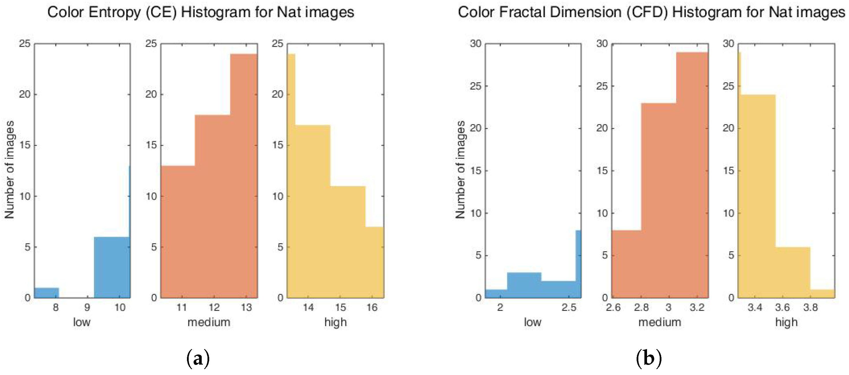
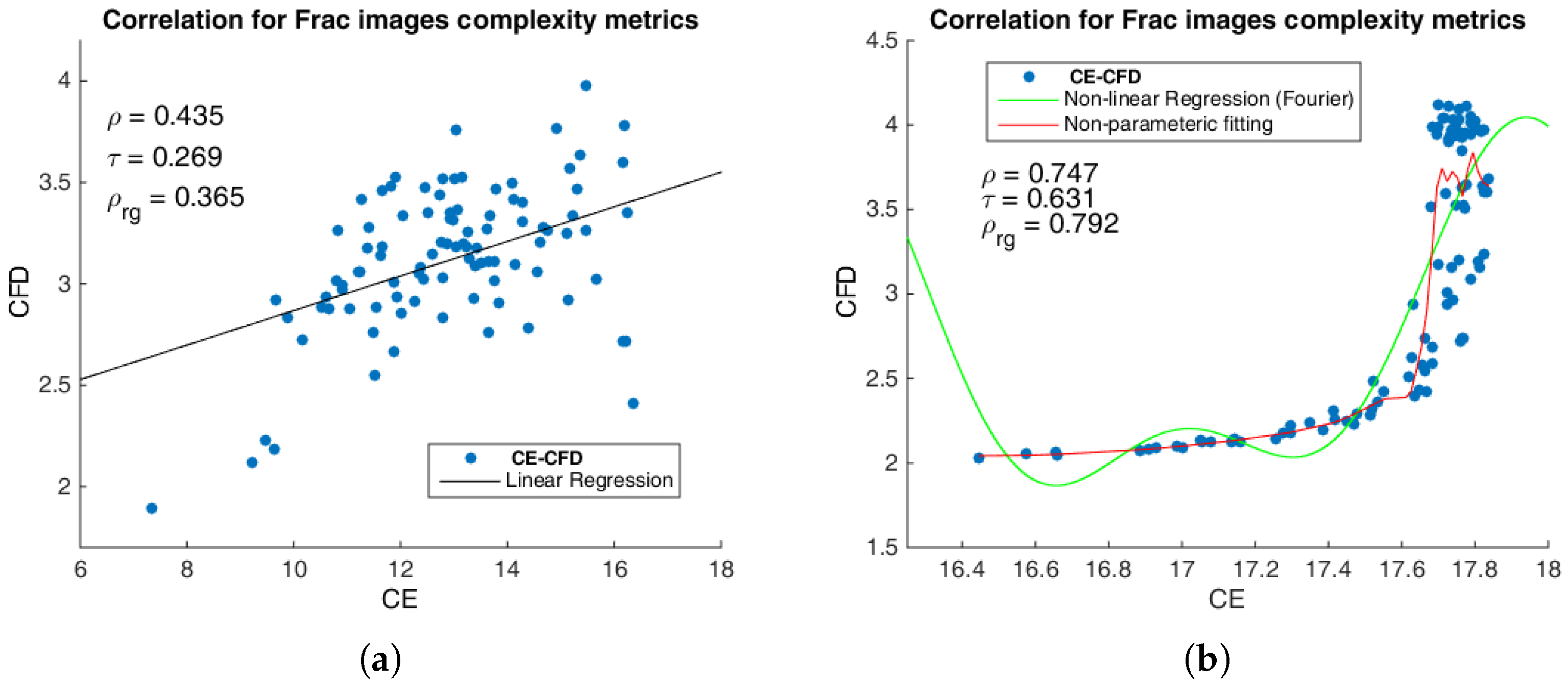
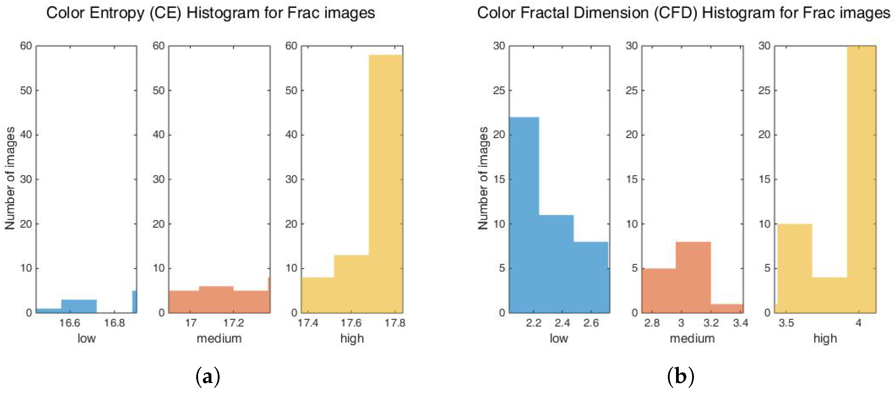
The natural images exhibit a complexity measure comprised between 7.33 and 16.37 for color entropy (Figure 2a), and in the range 1.89–3.98 for color fractal dimension (Figure 2b), with a Pearson correlation coefficient between CE and CFD of , expressing no significant correlation (also by non-linear measures: Kendall’s Tau and Spearman’s rank ), which is confirmed by the disperse distribution of points, as seen in Figure 3a. The fractal images contain between 16.45 and 17.84 CE values (Figure 4a) and between 2.03 and 4.12 CFD (Figure 4b), with a significant CE–CFD non-linear correlation of and (Figure 3b), such as CFD increases, as with an increase of CE, indicating that more texture colors increases the complexity.
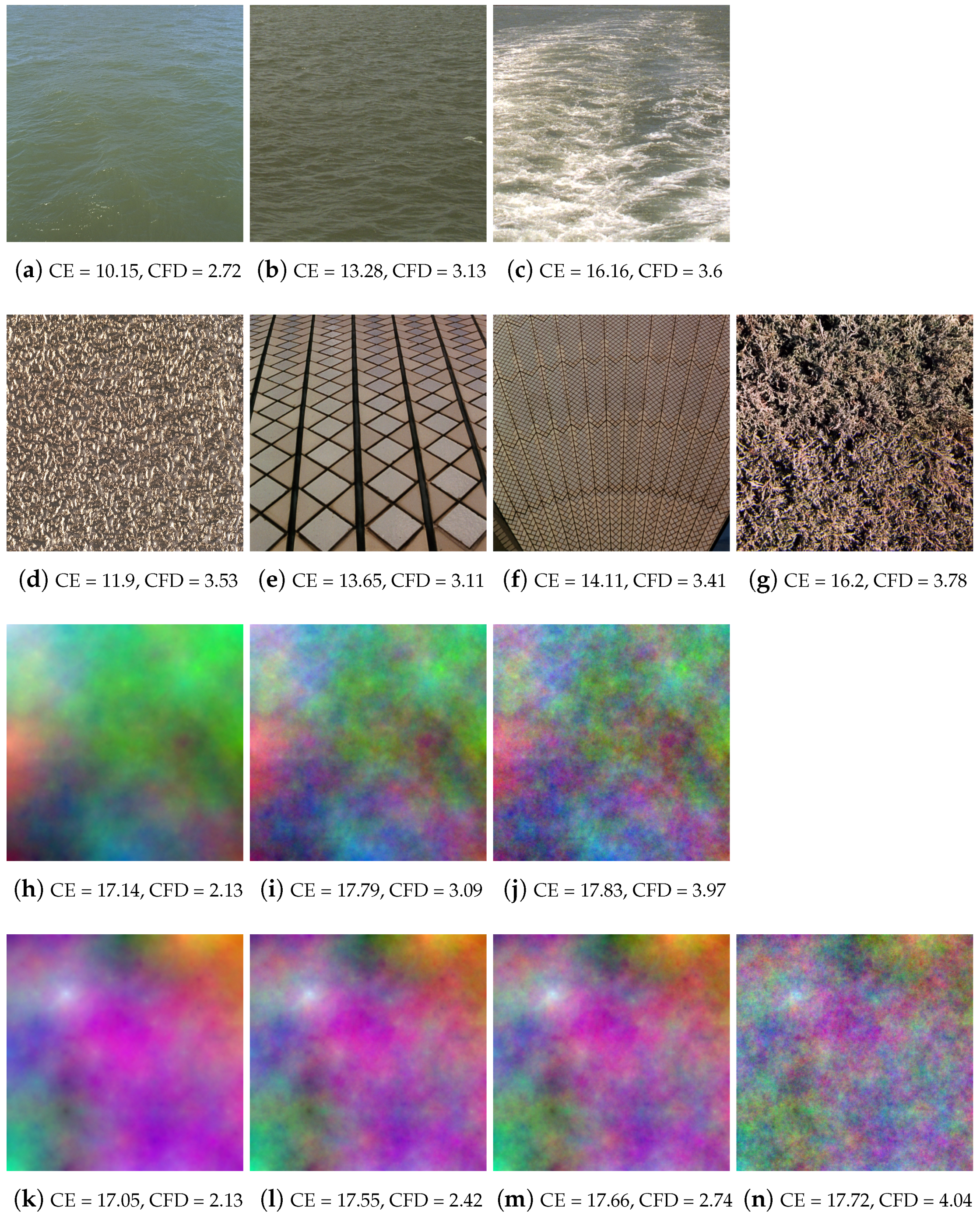
These facts can be easier understood if we look over some texture examples, as, for example, in Figure 5, the CE and CFD values are gradually increasing together as with a higher level of complexity for both natural and fractal textures, however this is not a general rule, as seen in Figure 5d–g, where, for some Nat image structures, when CE increases CFD varies differently. Therefore, not only the color amount influence complexity, but also the distribution of the elements, which is an important distinction to note between the random generated synthetic fractal structures for color fractal images and the natural occurring structure arrangements for color natural images. On this line, entropy is not a sufficient measure taken alone when expressing complexity, as also shown in [36]. That being said, when aiming to complexity by mathematical measures, contributions from both CE and CFD should be considered with appropriate weighting, depending on the content of the texture.
In the following, we investigate the correlations between the CE and CFD levels versus participants scoring. For significance, we refer to the Pearson Correlation Table of Critical Values [67], in relation to the respective amount of data points (97 Nat images and 99 Frac images). Therefore, we consider the threshold of for correlation, with a significance level of 5%, = 0.05 [68,69]. For a viable comparison with participants answers on complexity levels (1—low, 2—medium, 3—high), we consider three levels of complexity equally divided based on CE values and separately on CFD values for Nat and Frac images, as shown in the table below (Table 2).
7.2.1. Natural Images
When analysing the percentage of resemblance between the complexity levels expressed by image analysis measures and individuals as a response to natural textures, only a few cases are detected as highly significant: CE–P1 (), CE–P5 () and CFD–P3 (). While, between participants answers, strong positive correlations are observed () in half of the cases (54%), with highest correlations between P1 and P5, P3 and P4 (Table 3). No significant correlation is observed for P2 in all cases, as explained by main own subjective evaluation criteria based on sensations (e.g., 3D sensations, including texture vastness and volume information).
7.2.2. Fractal Images
When considering Frac images, significant correlations were observed (), except P2 and P7 participants—who considered the textures predominantly as medium complexity. Almost half of the participants correlate in answers (46%) and further, participants answers correlate more with the CFD levels, as compared to CE levels (Table 4). For five subjects, there is a significant resemblance between the participants’ answers and the complexity levels expressed by CE and CFD: CE–P3 (), CE–P4 (), CE–P8 (), CFD–P1 (), CFD–P4 (), and CFD–P6 (). Between participants, the highest correlations are observed between P1 and P3 () and P1 and P4 (). Significant negative correlations are observed for participant P5 in relation to the computed measures and other participants, and it is explained by the fact that the participant merely considered low complexity for the fractal textures, based on personal reasoning, attractiveness, emotions, memories, and imagination, which were not felt for participant P5 when viewing the synthetic fractal textures due to the lack of relation to known forms.
These results highlight that the internal reasoning on complexity is subjective for individuals, and the variations between individuals are higher for Frac images, probably because the texture contained does not relate to known forms and the decision on complexity involves more imaginatory actions requiring longer time and intense processes, which may obstruct the observer in its reasoning process. Further, for Frac images, participant reasoning is closer to the color fractal dimension estimation, then to color entropy, which is curious to observe since CE and CFD measures are highly correlated, as seen in Figure 4b. The subjective responses not detected as significantly correlated with the analysis measures, most probably relate to the other human internal reasoning mechanisms, as described in Section 7.1, which does not relate to criteria detectable by image texture analysis.
7.3. EEG Experiment Analysis
In the following, we complement the texture complexity evaluation with deep dive into the neural responses (ERP and power spectrum) and analyze the correlations with the image complexity measures and subjective evaluation. For the ERP trials, we consider the complexity levels as labels, as expressed by CE, CFD (Table 2), or participants’ answers and group the trials separately based on the them.
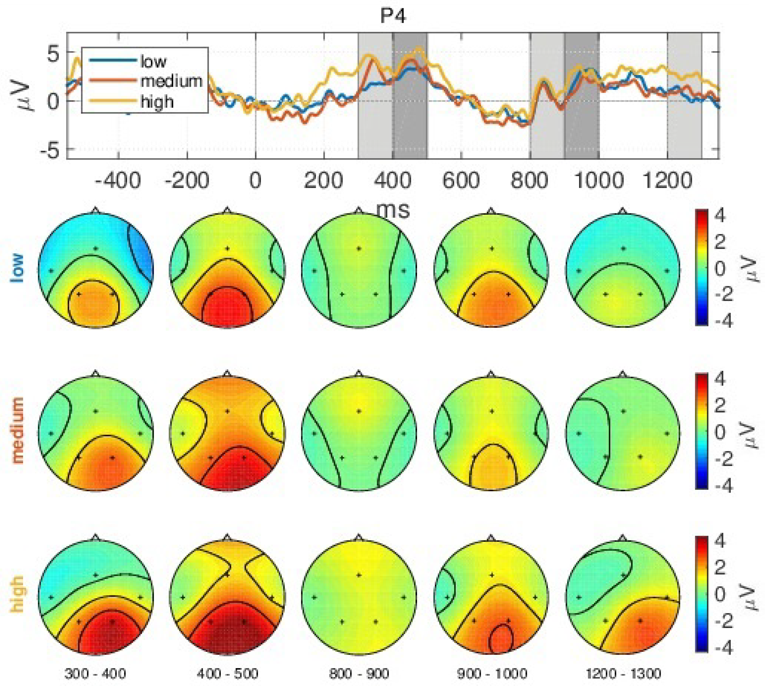
When considering ERPs, as also observed in our previous work [48], the visual perception and cognitive reasoning on complexity influenced by the ERP paradigm generates two discriminative groups of peaks (see e.g., Figure 6). One group is observed from 300 ms after the stimuli is presented (0 ms) comprising of a P200 potential (appearing at 300–400 ms), which varies in amplitude according to the level of complexity perception, relating to the visual perception of the texture and preparation for the cognitive task of complexity level decision, and it is followed by a P300 potential (400–600 ms) representing reasoning processes, which also varies in amplitude and extends differently in time on a trial base, depending on the respective texture complexity reasoning. The second group of peaks (800–1300 ms) appears at 300 ms after the presentation of the relaxation screen (single grey image), and it is comprised by a P200 potential that is equal in amplitude for all levels of textural complexity processing, followed by a P300, which varies in amplitude and it has a prolongued duration that is influenced by the ongoing neural processes relating to an extended thought process for complexity decision.
For the correlation analysis, we investigate whether the amplitude of the N3/N300 (min value from 350–450 ms), P3/P300 (max from 400–500 ms) and second P300b/P3b (mean from 1250–1350 ms) vary proportionally with the complexity values (CE, CFD) or participants answers [70].
For power spectrum, we consider the maximum value in the frequency band (6–12 Hz) and the mean value within the band (18–22 Hz). A stronger power of the signal should be related to a higher level of complexity, if correlated.
We present the significantly correlated cases as a sresponse to Nat and Frac textures in the table below (Table 5) and discuss them further.
7.3.1. Natural Images
ERPs vs. CE
First, it is important to note the CE complexity levels distributions among images: low: 34% of images; medium: 34%; and, high: 32%, which are balanced between classes, so we can rely on Grand Average ERPs interpretation, since unbalanced classes could influence the mean in favor of the class with more trials.
The Grand Average (GA) amplitudes of the ERPs at channel P4, as shown in top plot in Figure 6, is gradually increasing once with an increased level of complexity, as expressed by CE. The scalp maps likewise show increased activity in the parietal area (P3, P4 channels) for the P200 peak (300–400 ms), P300 peak (400–500 ms), and second P3b (1200–1300 ms). We observe that, for a lower level of complexity (low, medium), the neural activity focuses also in the visual area probably relating to more aspects of attention and visualisation [71,72], while, dor a complex level, only the parietal area is activated involving a more complex decision and it is right lateralized, tending to suggest imagery processes [73,74,75,76].
However, no significant correlation was detected here in relation to CE levels, which might probably be due to few high correlations between participants answers and computed measures, as seen in Table 3. In addition, the ERP amplitude varies from trial-to-trial due to many factors, and a direct proportional connection to the increase in CE values is therefore hard to detect.
ERPs vs. CFD
The CFD complexity levels distributions: low: 33%; medium: 35%; high: 32% (balanced).
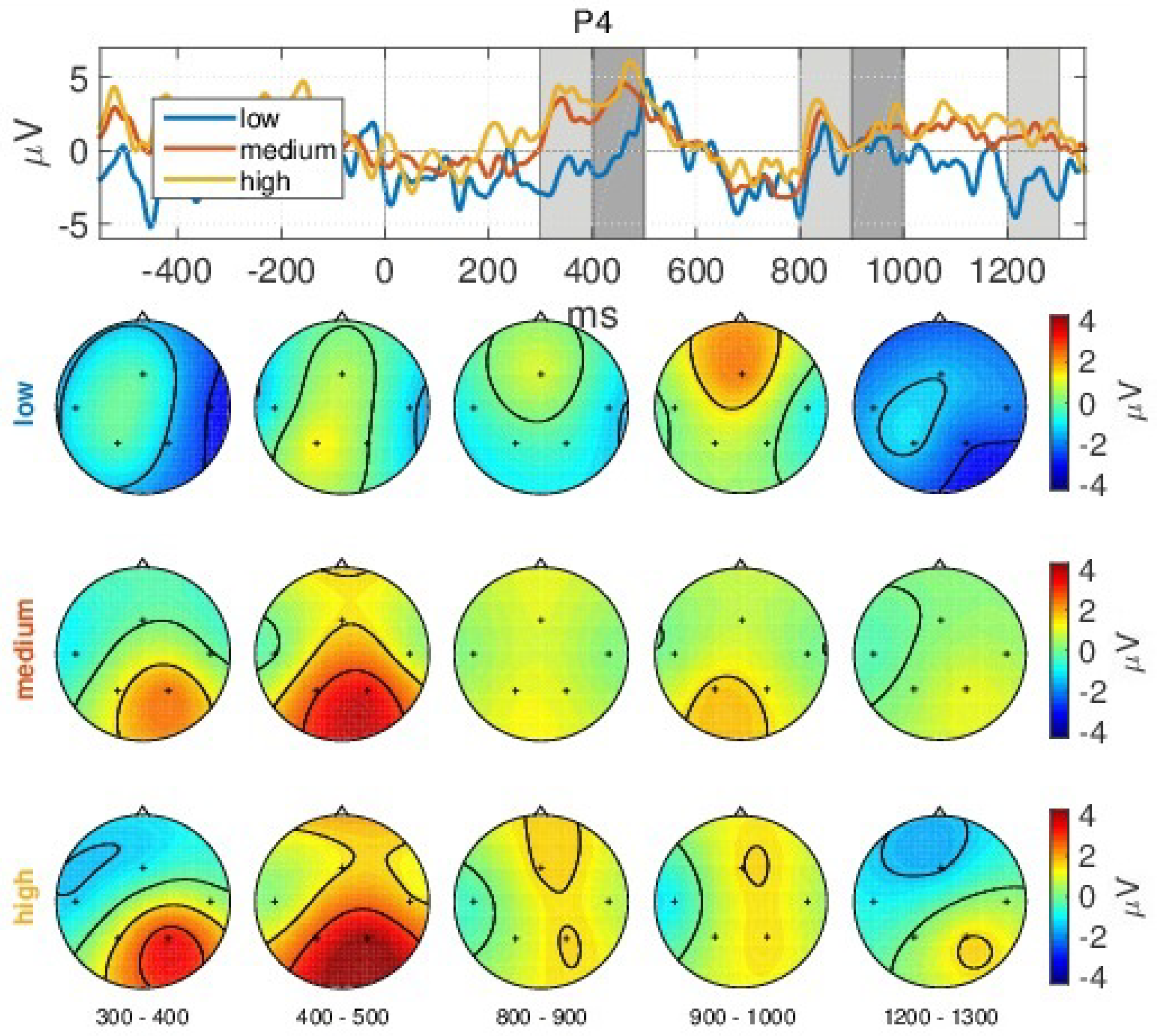
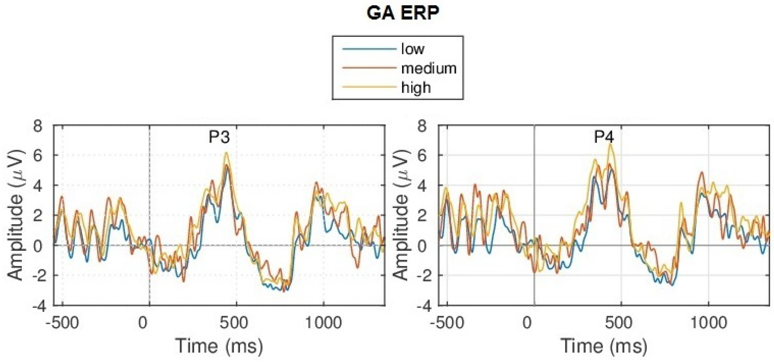
The ERP responses in time for Nat images according to the CFD levels as shown in Figure 7 indicate a gradual increase in amplitude, proportional with a higher level of complexity (low CFD complexity—blue; medium—red; high—orange), visible also over all channels (Figure A1 in Appendix A); however, only N300 at the P4 channel correlate significantly () with the CFD values considering the trial averages across participants. The gradual increase in amplitude and spatial activity can be seen in Figure 7, with more parietal activity as with a complex level and less frontal activity (only visible for P3 peak at 400–500 ms).
ERPs vs. Participants Scoring
First, we note participants’ complexity levels distributions, where, for:
- -
- participant P1: 44.3% images are considered as low complexity, 40.2% as medium: and 15.5% as high (resulting in unbalanced classes),
- -
- participant P2: low: 18.6%; medium: 67%; high: 14.4% (unbalanced),
- -
- participant P3: low: 0%; medium: 37.1%; high: 62.9% (unbalanced),
- -
- participant P4: low: 20.6%; medium: 13.4%; high: 66% (unbalanced),
- -
- participant P5: low: 27.8%; medium: 43.3%; high: 28.9% (unbalanced),
- -
- participant P6: low: 2%; medium: 25.8%; high: 72.2% (unbalanced),
- -
- participant P7: low: 1%; medium: 22.7%; high: 76.3% (unbalanced),
- -
- participant P8: low: 6.2%; medium: 68%; high: 25.8% (unbalanced).
When grouping the ERPs based on participants levels (Figure 8), the effect of complexity is visible on grand average, with a higher amplitude for P300–400 and a higher parietal activity, and, for the second P3b, we observe a higher activity for the P4 channel for a more complex level, and a more negative activity for a lower level. However, since ERP grand averages can be influenced by unbalanced classes that are given by the subjective responses, we look further into specific correlations. Analysing for each participant, the effect is anti-correlated for participant P5 at the P3 channel (N300: ; P300: ; 2nd P3b: ), and, for participant P7, also at P3 channel (2nd P3b: ), and correlated for participant P8 at P4 channel, for the P300 and the 2nd P3b peaks with and , respectively.
Spectral Activity vs. CE
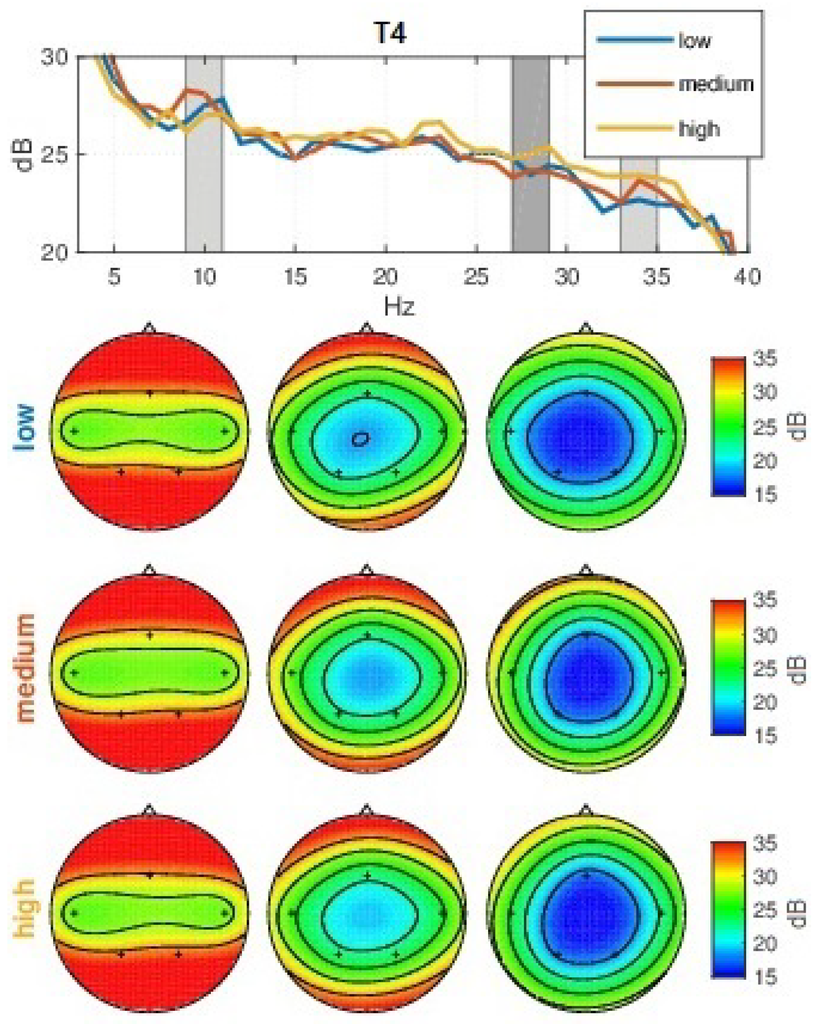
Now, looking over the GA spectral activity shown in Figure 9 at the P4 channel, we observe a gradual increase in power after 22 Hz, once with an increased level of processing. The opposite effect was observed for the P3 channel, being significantly anti-correlated for participant P8 for the and bands (, ). No important difference is observed when considering scalp activity.
Spectral Activity vs. CFD
When comparing the power spectrum with the CFD values, correlations and anti-correlations are observed for half of the participants as shown below:
- -
- participant P2: Ch P3, band,
- -
- participant P3: Ch T4, band,
- -
- participant P6: Ch T4, band, ; band,
- -
- participant P7: Ch P4, band, ; Ch T4, band,
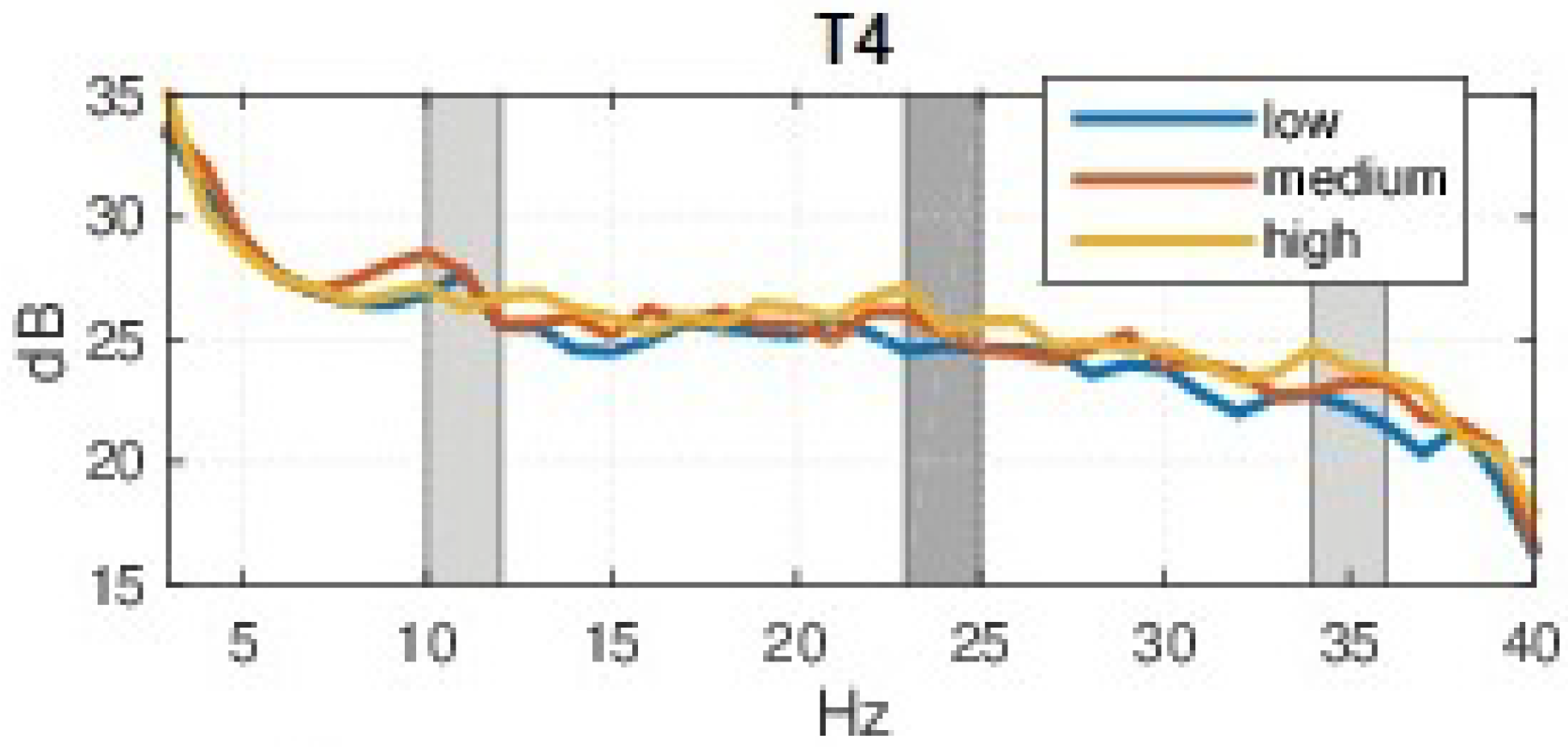
The correlation effect in the power spectrum as with CFD levels can also be observed on grand average, in Figure 10, for channel T4.
7.3.2. Fractal Images
The effect of complexity over the ERPs, in relation to CE, CFD, and participants scoring is also observed, in parts, for the Frac images, as shown in the following.
ERPs vs. CE
CE complexity levels distributions: low: 6.1%; medium: 14.1%; and, high: 79.8% (unbalanced).
Relating with CE values, few cases are detected as significantly anti-/correlated for ERPs:
- -
- participant P1: Ch P3, N300, ; P300, ; 2nd P3b ; Ch P4, P300, ; 2nd P3b
- -
- participant P4: Ch P3, N300, ; 2nd P3b ; Ch P4, P200, ; 2nd P3b
- -
- participant P6: Ch P3, P300,
ERPs vs. CFD
CFD complexity levels: low: 41.4%; medium: 14.1%; high: 44.5% (unbalanced).
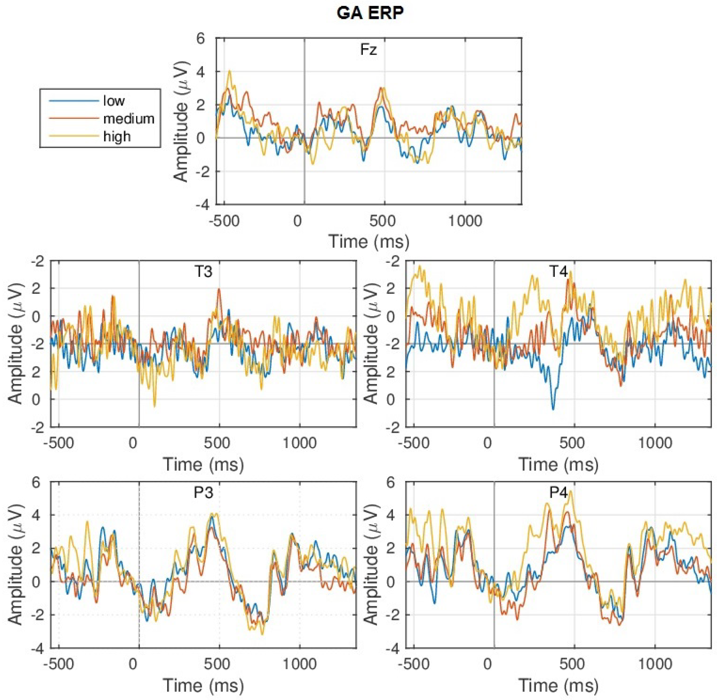
In relation with the CFD levels, as shown in Figure 11 for the P3 channel, ERPs are significantly correlated on grand average for P300 with and 2nd P3b , and for two participants at the P3 and P4 channels, as shown below:
- -
- participant P4: Ch P3, N300, ; 2nd P3b ; Ch P4, N300, ; 2nd P3b
- -
- participant P8: Ch P3, P300, ; Ch P4, P300,
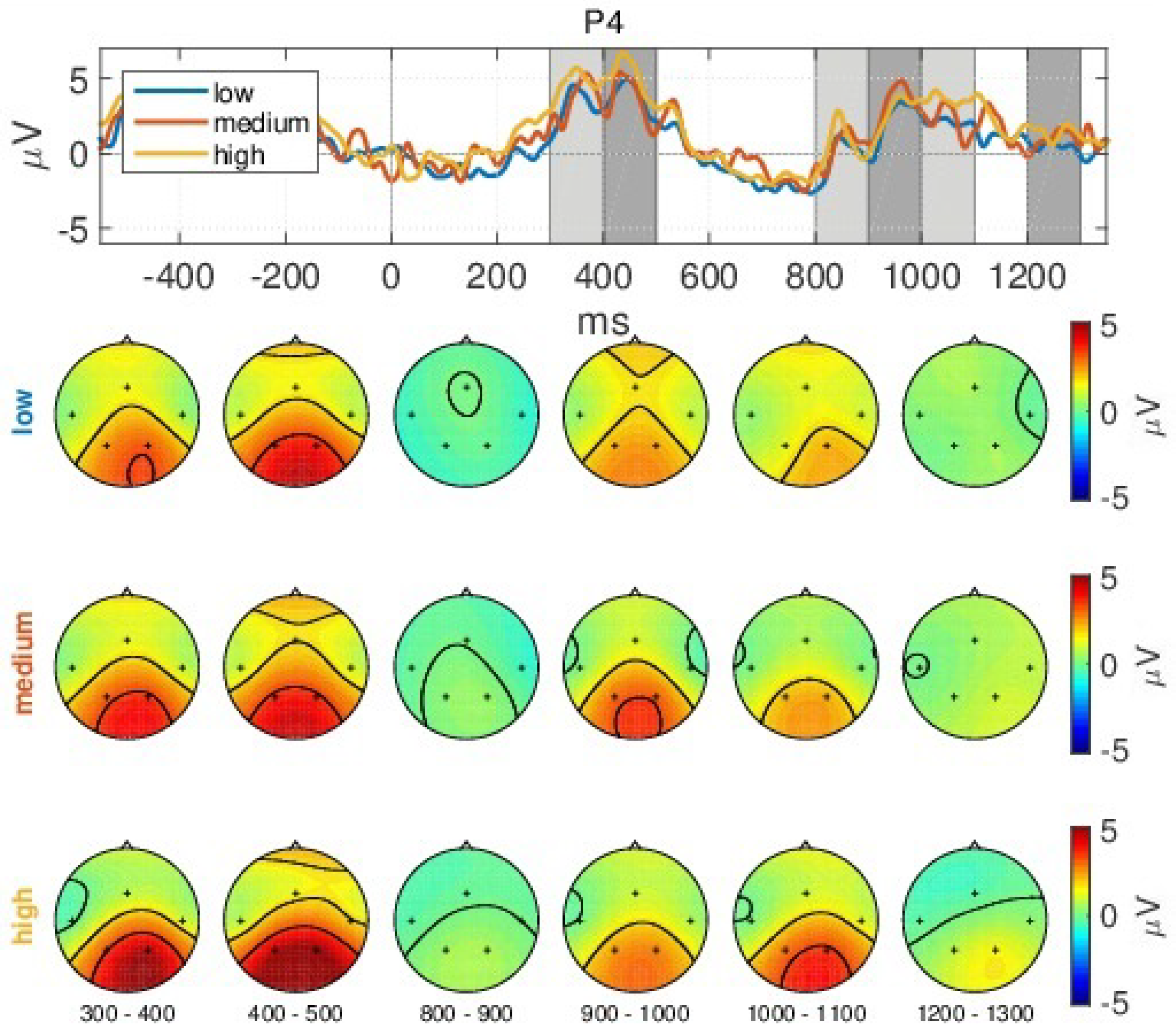
On grand average, the ERPs cannot be easily differentiated, as seen in Figure 11. Here, the high complexity level only induces a 1 V higher ERP, as compared to low and medium classes. The right plot shown in Figure 11 as for P4 channel, can be further seen in extension, in the top plot of Figure 12 which considers in addition, the spatial activity. Here, spatial activity shows an interesting phenomena at the 900–1000 ms time point, where the medium class has higher activation when compared to the high class. However, this effect is not maintained within the neighboring intervals.
Spectral Activity vs. Participants Scoring
participants complexity levels distributions:
- -
- P1: low: 30.3%; medium: 41.4%; high: 28.3% (∼balanced).
- -
- P2: low: 4%; medium: 87.9%; high: 8.1% (unbalanced).
- -
- P3: low: 0%; medium: 63.6%; high: 36.4% (unbalanced).
- -
- P4: low: 25.3%; medium: 30.3%; high: 44.4% (∼balanced).
- -
- P5: low: 81.8%; medium: 10.1%; high: 8.1% (unbalanced).
- -
- P6: low: 61.6%; medium: 25.3%; high: 13.1% (unbalanced).
- -
- P7: low: 0%; medium: 100%; high: 0% (unbalanced).
- -
- P8: low: 1%; medium: 13.1%; high: 85.9% (unbalanced).
Investigating the power spectrum in relation with subjective scoring (Figure 13), we observe an increase in power with an increased level of complexity from 20 Hz onwards. However, no significant correlations are observed.
Overall, more significant positive correlations were detected for participants in relation to the Nat textures. Participants P3 and P8 show positive correlations in neural signals for Nat cases, while P4 and P8 exhibit positive correlations for Frac cases. The highest correlations detected in relation to CE and, respectively, CFD for participant P4 for the Frac case are supported by the complexity criteria used in the thought processes that refer solely to texture characteristics, namely: colors, distribution, and spatial arrangement (disorder vs. order), which are expressed by CE and, respectively, CFD analysis measures.
For participants P1, P2, P5, P6, P7, and P8, anti-correlation results are detected for neural signals, which suggests that a different rationale was involved in deciding on the complexity level, with no direct connection to the amount of colors of texture structure; a fact that is sustained by the participants’ descriptions during the subjective evaluation, relying on external criteria as the primary factors for deciding on complexity, such as first impression, sensations, mood induced, and so on.
In general, we observed that, when considering complexity evaluation, the CFD values tend to correlate more with the neural responses than with CE. However, we observed that, there is not a good correlation between the brain responses (ERPs or power spectrum activity) with the computed measures in all cases, meaning that the neural oscillations are not proportionate with an increase in texture colors or structure complexity, while the internal thought processes differ from the known complexity criteria that are based on texture characteristics. In addition, it is curious that not even the subjective scoring correlated entirely with the neural responses (ERPs and power). This suggests that some other factors contribute to the influence in amplitude and power and not necessarily the complexity levels. In this regard, the duration and latency of the ERPs should be also considered to evaluate complexity decision.
8. Discussion
The complementary study on the subjective responses in addition to the neural signals analysis revealed that there is less correlation agreement between participants, and each interpretation is more or less unique. However, the CE and CFD measures correlate considerably with the majority of participants’ responses, especially for the low, mid, or high complexity for natural/synthetic fractals. The EEG analysis showed that various potential levels or spectral responses are partially in agreement with the three levels of complexity. This is due to different reasoning processes among individuals who use distinct complexity criteria for the decision. In addition, the synthetic fractals that look similar to chaotic structures induces further difficulty and uncertainty on the decision, being supplemented by the free choice for evaluating complexity, since no formal definition of complexity was suggested to the participants. This opinion is confirmed by the high ERP activity, even in the later interval (800–1200 ms) [77], suggesting a complex and a prolonged continuous background process, while also briefly showing a negative ERP over the prefrontal cortex for P300 (300–400 ms) in Figure 6 for the high complexity level suggesting indecisiveness [78]. Furthermore, the images’ textural representations might be affected by uncertainties or inaccuracies when considering the edges of textural forms. For these cases, fuzzy image pre-processing [79] can be applied to reduce vagueness and enhance PSNR—a technique that has been been shown to be successful for X-ray imagery, for example [80].
9. Conclusions and Future Developments
This paper is a follow up of the investigations carried out in [48], and it contributes to the understanding of the relation between visual complexity perception and the computational visual complexity expressed by image analysis and it provides the directions for multi-scale studies with a higher number of participants and more types of textures. We have shown that we were able to extract information, even with a less informative five-channel system with wireless connection and make some neurophysiological interpretation in this particular context of visual perception and reasoning, highlighting the feasibility of using such settings for further use in research, clinical, or ambulatory environments until commercially good quality systems will be available on the market on a large scale. We have further highlighted that different perceived aspects of an image intervene in the assessment of image complexity, as previous works agreed [26].
A follow-up study is necessary for complexity evaluations, in order to analyze each complexity criteria that go beyond the textural properties and how much each factor contributes to the final decision on complexity. Therefore, we leave open the quest to further explore the human brain, directly tapping the corresponding relations between imagination, memory, emotions, and user specific understanding of complexity based on own background, the stock of knowledge, and previous experiences [81], which influence the reasoning, perception, and understanding of complexity, and further integrate the contributing top-down mechanisms in a vast model of complexity assessment. In terms of image complexity measures, since color entropy and color fractal dimension are not the only measures for describing texture complexity [82,83,84,85,86], measures, like lacunarity (which measures the gaps distributions [87]), succolarity (which expresses the degree of filaments that allow percolation or flow through the texture [88,89]), and artistic complexity derived from neuroscience [84] could be further used for comparison.
Evaluating further complexity perception of textures could play a role not only in computer vision applications, and neuroscience, but also by establishing for example a performance evaluation for complexity reasoning could have an impact also for health investigations for evaluating cognitive decline.
Author Contributions
Conceptualization, I.E.N. and M.I.; Methodology, I.E.N. and M.I.; Software, I.E.N.; Validation, M.I.; Formal analysis, I.E.N.; Investigation, I.E.N.; Resources, M.I.; Data Curation, I.E.N. and M.I.; Writing—Original Draft Preparation, I.E.N.; Writing—Review & Editing, M.I.; Visualization, I.E.N. and M.I.; Supervision, M.I.; Project Administration, M.I.; Funding Acquisition, I.E.N. and M.I. All authors have read and agreed to the published version of the manuscript.
Funding
This research is part of the post-doctoral research project entitled PerPlex: ”Human brain perception on the spatio-chromatic complexity of fractal color images”, carried out at University Transilvania of Brasov (UniTBv), Romania and was funded by the National Council of Scientific Research (CNCS) Romania grant number CNFIS-FDI-2019-0324.
Institutional Review Board Statement
The study was conducted according to the guidelines of the Declaration of Helsinki, and approved by the ethical Committee of Medical Electronics and Computing Laboratory from the Faculty of Electronics, Telecommunications and Information Technology, University Politehnica of Bucharest.
Informed Consent Statement
Informed consent was obtained from all subjects involved in the study and the recorded data is completely anonymized.
Data Availability Statement
The recorded EEG data is available at http://0-dx-doi-org.brum.beds.ac.uk/10.6084/m9.figshare.13489215 [50].
Acknowledgments
We would like to thank our colleagues from University Transilvania of Braşov for offering us the opportunity to use the EEG H&S system (during 2019–2020), namely to: MOŞOI Adrian Alexandru from Faculty of Physical Education and Mountain Sports and CAZAN Ana-Maria from Faculty of Psychology and Education Sciences.
Conflicts of Interest
The authors declare no conflict of interest.
Abbreviations
The following abbreviations are used in this manuscript:
| EEG | Electroencephalography |
| BCI | Brain-Computer Interfaces |
| ERPs | Event-Related Potentials |
| CFD | Color Fractal Dimension |
| CE | Color Entropy |
| CFD | Color Fractal Dimension |
| Uni | one-color image |
| Nat | color natural texture image |
| Frac | color fractal texture image |
| P1, P2, P3, P4, P5, P6, P7, P8 | participants indices |
| Pearson correlation | |
| Kendall’s Tau correlation | |
| Spearman’s rank correlation | |
| GA | Grand Average (mean over all participants and trials) |
| P200 | positive peak of ERP potential appearing 200 ms after stimulus |
| P3/P300 | ERP (positive peak) appearing 300 ms after stimulus |
| N3/N300 | ERP (negative peak) appearing 300 ms after stimulus |
| P300b/P3b | ERP cognitive component (positive peak) appearing later >300 ms |
| alpha frequency EEG band (6–12 Hz) | |
| beta frequency EEG band (18–22 Hz) | |
| sbj. | subjective evaluation scoring |
| ex. CE–N3 | CE measure versus N3 potential |
| Ch P3, Ch P4 | EEG channels from brain parietal area |
| Ch T3, Ch T4 | EEG channels from brain temporal area |
| Ch Fz | EEG channels from brain frontal area |
Appendix A
Figure A1.
Grang Average (GA) ERPs for Nat images on 3 complexity levels according to CFD: low (blue), medium (red) and high (orange) complexity, for all channels.
Figure A1.
Grang Average (GA) ERPs for Nat images on 3 complexity levels according to CFD: low (blue), medium (red) and high (orange) complexity, for all channels.

References
- Poltavski, D.V. The use of single-electrode wireless EEG in biobehavioral investigations. In Mobile Health Technologies; Springer: Berlin, Germnay, 2015; pp. 375–390. [Google Scholar]
- Casson, A.J. Wearable EEG and beyond. In Biomedical Engineering Letters; Springer: Berlin, Germany, 2019; Volume 9, pp. 53–71. [Google Scholar]
- Allison, B.Z.; Dunne, S.; Leeb, R.; Millán, J.R.; Nijholt, A. Recent and upcoming BCI progress: Overview, analysis, and recommendations. In Towards Practical Brain-Computer Interfaces; Springer: Berlin, Germany, 2012; pp. 1–13. [Google Scholar]
- Hinrichs, H.; Scholz, M.; Baum, A.K.; Kam, J.W.Y.; Knight, R.T.; Heinze, H.J. Comparison between a wireless dry electrode EEG system with a conventional wired wet electrode EEG system for clinical applications. Sci. Rep. 2020, 10, 1–14. [Google Scholar] [CrossRef]
- Guger, C.; Krausz, G.; Allison, B.Z.; Edlinger, G. Comparison of dry and gel based electrodes for P300 brain–computer interfaces. Front. Neurosci. 2012, 6, 60. [Google Scholar] [CrossRef] [Green Version]
- O’Sullivan, M.; Temko, A.; Bocchino, A.; O’Mahony, C.; Boylan, G.; Popovici, E. Analysis of a low-cost EEG monitoring system and dry electrodes toward clinical use in the neonatal ICU. Sensors 2019, 19, 2637. [Google Scholar] [CrossRef] [Green Version]
- Jackson, G.; Radhu, N.; Sun, Y.; Tallevi, K.; Ritvo, P.; Daskalakis, Z.J.; Grundlehner, B.; Penders, J.; Cafazzo, J.A. Comparative Evaluation of an Ambulatory EEG Platform vs. Clinical Gold Standard. In Proceedings of the 2013 35th Annual International Conference of the IEEE Engineering in Medicine and Biology Society (EMBC), Osaka International Convention Center, Osaka, Japan, 3–7 July 2013; pp. 1222–1225. [Google Scholar]
- Paszkiel, S.; Hunek, W.; Shylenko, A. Project and Simulation of a Portable Device for Measuring Bioelectrical Signals from the Brain for States Consciousness Verification with Visualization on LEDs. In Proceedings of the International Conference on Automation, Warsaw, Poland, 2–4 March 2016; Springer: Cham, Switzerland, 2016; pp. 25–35. [Google Scholar]
- Mihajlović, V.; Grundlehner, B.; Vullers, R.; Penders, J. Wearable, wireless EEG solutions in daily life applications: What are we missing? IEEE J. Biomed. Health Inform. 2014, 19, 6–21. [Google Scholar] [CrossRef]
- Niedermeyer, E.; da Silva, F.H.L. Electroencephalography: Basic Principles, Clinical Applications, and Related Fields; Lippincott Williams & Wilkins: Philadelphia, PN, USA, 2005; pp. 1–13. [Google Scholar]
- Jackson, G. Towards a Wireless EEG System for Ambulatory Mental Health Applications. Master’s Thesis, University of Toronto, Toronto, ON, Canada, 2013. [Google Scholar]
- Noachtar, S.; Rémi, J. The role of EEG in epilepsy: A critical review. Epilepsy Behav. 2009, 15, 22–33. [Google Scholar] [CrossRef]
- Vidgeon, S.D.; Strong, A.J. Multimodal cerebral monitoring in traumatic brain injury. J. Intensive Care Soc. 2011, 12, 126–133. [Google Scholar] [CrossRef]
- Ziai, W.C.; Schlattman, D.; Llinas, R.; Venkatesha, S.; Truesdale, M.; Schevchenko, A.; Kaplan, P.W. Emergent EEG in the emergency department in patients with altered mental states. Clin. Neurophysiol. 2012, 123, 910–917. [Google Scholar] [CrossRef] [PubMed]
- Lenartowicz, A.; Loo, S.K. Use of EEG to diagnose ADHD. Curr. Psychiatry Rep. 2014, 16, 498. [Google Scholar] [CrossRef] [Green Version]
- Cavanagh, P. Visual cognition. Vis. Res. 2011, 51, 1538–1551. [Google Scholar] [CrossRef] [PubMed] [Green Version]
- Rosenholtz, R. Texture Perception. In Oxford Handbook of Perceptual Organization; Oxford University Press: Oxford, UK, 2014; Volume 167, p. 186. [Google Scholar]
- Sand, T.; Bjørk, M.H.; Vaaler, A.E. Is EEG a useful test in adult psychiatry? Tidsskr. Nor Laegeforen. 2013, 133, 1200–1204. [Google Scholar] [CrossRef] [PubMed] [Green Version]
- Boutros, N.N. The Electroencephalogram in the Management of Psychiatric Conditions. Psychiatr. Times 2013, 30. [Google Scholar]
- Hu, L.; Zhang, Z. Evolving EEG signal processing techniques in the age of artificial intelligence. Brain Sci. Adv. 2020, 6, 159–161. [Google Scholar] [CrossRef]
- Paszkiel, S.; Szpulak, P. Methods of acquisition, archiving and biomedical data analysis of brain functioning. In Proceedings of the International Scientific Conference BCI 2018 Opole, Opole, Poland, 13–14 March 2018; Springer: Cham, Switzerland, 2018; pp. 158–171. [Google Scholar]
- Yadav, A.K. Survey on content-based image retrieval and texture analysis with applications. Int. J. Educ. Res. 2014, 77, 41–50. [Google Scholar] [CrossRef]
- Ivanovici, M.; Coliban, R.M.; Hatfaludi, C.; Nicolae, I.E. Color Image Complexity versus Over-Segmentation: A Preliminary Study on the Correlation between Complexity Measures and Number of Segments. J. Imaging 2020, 6, 16. [Google Scholar] [CrossRef] [Green Version]
- Forsythe, A.; Sheehy, N.; Sawey, M. Measuring Icon Complexity: An Automated Analysis. In Behavior Research Methods, Instruments & Computers; Springer: Berlin, Germany, 2003; Volume 35, pp. 334–342. [Google Scholar]
- Reinecke, K.; Yeh, T.; Miratrix, L.; Mardiko, R.; Zhao, Y.; Liu, J.; Gajos, K.Z. Predicting users’ first impressions of website aesthetics with a quantification of perceived visual complexity and colorfulness. In Proceedings of the SIGCHI Conference on Human Factors in Computing Systems, Paris, France, 27 April–2 May 2013; pp. 2049–2058. [Google Scholar]
- Donderi, D.C. Visual complexity: A review. Psychol. Bull. 2006, 132, 73. [Google Scholar] [CrossRef] [Green Version]
- Huo, J. An Image Complexity Measurement Algorithm with Visual Memory Capacity and an Eeg Study. In Proceedings of the 2016 SAI Computing Conference (SAI), London, UK, 13–15 July 2016; pp. 264–268. [Google Scholar]
- Shafahi, A.; Huang, W.R.; Studer, C.; Feizi, S.; Goldstein, T. Are adversarial examples inevitable? arXiv 2018, arXiv:1809.02104. [Google Scholar]
- Kwon, H.; Kim, Y.; Yoon, H.; Choi, D. Selective audio adversarial example in evasion attack on speech recognition system. IEEE Trans. Inf. Forensics Secur. 2019, 15, 526–538. [Google Scholar] [CrossRef]
- Kwon, H.; Yoon, H.; Park, K.W. Acoustic-decoy: Detection of adversarial examples through audio modification on speech recognition system. Neurocomputing 2020, 417, 357–370. [Google Scholar] [CrossRef]
- Scha, R.; Bod, R. Computationele esthetica. Inf. Informatiebeleid 1993, 11, 54–63. [Google Scholar]
- Heylighen, F. The Growth of Structural and Functional Complexity during Evolution. In The Evolution of Complexity; KluwerAcademic: Dordrecht, The Netherlands, 1999; pp. 17–44. [Google Scholar]
- Guo, X.; Asano, C.M.; Asano, A.; Kurita, T.; Li, L. Analysis of texture characteristics associated with visual complexity perception. Opt. Rev. 2012, 19, 306–314. [Google Scholar] [CrossRef]
- Ciocca, G.; Corchs, S.; Gasparini, F. Genetic programming approach to evaluate complexity of texture images. J. Electron. Imaging 2016, 25, 061408. [Google Scholar] [CrossRef]
- Chi, J.; Yu, X.; Zhang, Y.; Wang, H. A novel local human visual perceptual texture description with key feature selection for texture classification. Math. Probl. Eng. 2019. [Google Scholar] [CrossRef]
- Ivanovici, M.; Richard, N. Entropy Versus Fractal Complexity for Computer-Generated Color Fractal Images. In Proceedings of the 4th CIE Expert Symposium on Colour and Visual Appearance, Prague, Czech Republic, 6–7 September 2016; pp. 432–437. [Google Scholar]
- Kisan, S.; Mishra, S.; Mishra, D. A Novel Method to Estimate Fractal Dimension of Color Images. In Proceedings of the 11th International Conference on Industrial and Information Systems (ICIIS 2016), Roorkee, India, 3–4 December 2016; pp. 692–697. [Google Scholar]
- Zunino, L.; Ribeiro, H.V. Discriminating image textures with the multiscale two-dimensional complexity-entropy causality plane. Chaos Solitons Fractals 2016, 91, 679–688. [Google Scholar] [CrossRef] [Green Version]
- Perkiö, J.; Hyvärinen, A. Modelling Image Complexity by Independent Component Analysis, with Application to Content-Based Image Retrieval. In Proceedings of the International Conference on Artificial Neural Networks, Munich, Germany, 17–19 September 2019; Springer: Berlin/Heidelberg, Germany, 2019; pp. 704–714. [Google Scholar]
- Panigrahy, C.; Seal, A.; Mahato, N.K. Fractal dimension of synthesized and natural color images in lab space. Pattern Anal. Appl. 2020, 23, 819–836. [Google Scholar] [CrossRef]
- Ciocca, G.; Corchs, S.; Gasparini, F. Complexity Perception of Texture Images. In Proceedings of the International Conference on Image Analysis and Processing, Genova, Italy, 7–11 September 2015. [Google Scholar]
- Hagerhall, C.M.; Laike, T.; Taylor, R.P.; Küller, M.; Küller, R.; Martin, T.P. Investigations of human eeg response to viewing fractal patterns. Perception 2008, 37, 1488–1494. [Google Scholar] [CrossRef] [PubMed]
- Taylor, R.; Spehar, B.; Hagerhall, C.; Van Donkelaar, P. Perceptual and physiological responses to jackson pollock’s fractals. Front. Hum. Neurosci. 2011, 5, 60. [Google Scholar] [CrossRef] [Green Version]
- Corchs, S.E.; Ciocca, G.; Bricolo, E.; Gasparini, F. Predicting complexity perception of real world images. PLoS ONE 2016, 11, e0157986. [Google Scholar]
- Gartus, A.; Leder, H. Predicting perceived visual complexity of abstract patterns using computational measures: The influence of mirror symmetry on complexity perception. PLoS ONE 2017. [Google Scholar] [CrossRef] [PubMed] [Green Version]
- Rahane, A.A.; Subramanian, A. Measures of Complexity for Large Scale Image Datasets. In Proceedings of the 2020 International Conference on Artificial Intelligence in Information and Communication (ICAIIC), Fukuoka, Japan, 19–21 February 2020; pp. 282–287. [Google Scholar]
- Russakoff, D.B.; Tomasi, C.; Rohlfing, T.; Maurer, C.R. Image Similarity using Mutual Information of Regions. In Proceedings of the European Conference on Computer Vision, Prague, Czech Republic, 11–14 May 2004; pp. 596–607. [Google Scholar]
- Nicolae, I.E.; Ivanovici, M. Preparatory Experiments Regarding Human Brain Perception and Reasoning of Image Complexity for Synthetic Color Fractal and Natural Texture Images via EEG. Appl. Sci. 2021, 11, 164. [Google Scholar] [CrossRef]
- Ivanovici, M. Fractal Dimension of Color Fractal Images With Correlated Color Components. IEEE Trans. Image Process. 2020, 29, 8069–8082. [Google Scholar] [CrossRef]
- Nicolae, I.E. PerPlex EEG.zip. Dataset. Figshare. 2020. Available online: https://figshare.com/articles/dataset/PerPlex_EEG_zip/13489215/1 (accessed on 30 April 2021).
- Blankertz, B.; Acqualagna, L.; Dähne, S.; Haufe, S.; Schultze-Kraft, M.; Sturm, I.; Ušćumlic, M.; Wenzel, M.A.; Curio, G.; Müller, K.R. The berlin brain-computer interface: Progress beyond communication and control. Front. Neurosci. 2016, 10, 530. [Google Scholar] [CrossRef] [Green Version]
- Shannon, C.A. Mathematical Theory of Communication; Nokia Bell Labs: Holmdel, NJ, USA, 1948; Volume 318, pp. 379–423. [Google Scholar]
- Ivanovici, M.; Richard, N. Fractal dimension of color fractal images. IEEE Trans. Image Process. 2011, 20, 227–235. [Google Scholar] [CrossRef] [PubMed]
- Blackburn, S. How to ID Lion. Mara Predator Project 2009. Available online: http://marapredatorproject.blogspot.com/2009/01/how-to-id-lion.html (accessed on 30 April 2021).
- Humeau-Heurtier, A. The multiscale entropy algorithm and its variants: A review. Entropy 2015, 17, 3110–3123. [Google Scholar] [CrossRef] [Green Version]
- Zhou, E.Y.; Damiano, C.; Wilder, J.; Walther, D.B. Measuring complexity of images using Multiscale Entropy. J. Vis. 2019, 19, 96a. [Google Scholar] [CrossRef]
- Mejia, J.; Ochoa, A.; Mederos, B. Reconstruction of PET images using cross-entropy and field of experts. Entropy 2019, 21, 83. [Google Scholar] [CrossRef] [PubMed] [Green Version]
- Song, S.; Jia, H.; Ma, J. A Chaotic Electromagnetic Field Optimization Algorithm Based on Fuzzy Entropy for Multilevel Thresholding Color Image Segmentation. Entropy 2019, 21, 398. [Google Scholar] [CrossRef] [PubMed] [Green Version]
- Borowska, M. Entropy-based algorithms in the analysis of biomedical signals. Studies in Logic. Gramm. Rhetor. 2015, 43, 21–32. [Google Scholar] [CrossRef] [Green Version]
- Li, B.; Shu, H.; Liu, Z.; Shao, Z.; Li, C.; Huang, M.; Huang, J. Nonrigid Medical Image Registration Using an Information Theoretic Measure Based on Arimoto Entropy with Gradient Distributions. Entropy 2019, 21, 189. [Google Scholar] [CrossRef] [PubMed] [Green Version]
- Mandelbrot, B.B. The Fractal Geometry of Nature; WH freeman: New York, NY, USA, 1983; Volume 173. [Google Scholar]
- Barnsley, M.F.; Robert L Devaney, R.L.; Mandelbrot, B.B.; Peitgen, H.O.; Saupe, D.; Voss, R.F.; Fisher, Y.; McGuire, M. The Science of Fractal Images; Springer: Berlin, Germany, 1988; Volume 1, p. 312. [Google Scholar]
- Fisher, Y.; McGuire, M.; Voss, R.F.; Barnsley, M.F.; Devaney, R.L.; Mandelbrot, B.B. The Science of Fractal Images; Springer Science & Business Media: Berlin, Germany, 2012. [Google Scholar]
- Falconer, K. Mathematical foundations and applications. In Fractal Geometry; John Wiley & Sons: Hoboken, NJ, USA, 1990. [Google Scholar]
- Falconer, K. Fractal Geometry: Mathematical Foundations and Applications; John Wiley & Sons: Hoboken, NJ, USA, 2004. [Google Scholar]
- Voss, R.F. Random fractals: Characterization and measurement. In Scaling Phenomena in Disordered Systems; Springer: Berlin, Germany, 1991; pp. 1–11. [Google Scholar]
- Barbara, I.; Dean, S. Introductory Statistics. Available online: https://openstax.org/books/introductory-statistics/pages/12-6-outliers#eip-idm31993488 (accessed on 15 May 2020).
- Verma, J.P. Data Analysis in Management with SPSS Software; Springer Science & Business Media: Berlin, Germany, 2012. [Google Scholar]
- Nica, M. Principles of Business Statistics. Available online: http://www.opentextbooks.org.hk/ditatopic/9498 (accessed on 8 August 2020).
- Polich, J. Updating p300: An integrative theory of p3a and p3b. Clin. Neurophysiol. 2007, 118, 2128–2148. [Google Scholar] [CrossRef] [Green Version]
- Szczepanski, S.M.; Konen, C.S.; Kastner, S. Mechanisms of spatial attention control in frontal and parietal cortex. J. Neurosci. 2010, 30, 148–160. [Google Scholar] [CrossRef] [PubMed]
- Basile, L.F.H.; Sato, J.; Alvarenga, M.Y.; Nelson, H.J.; Pasquini, H.A.; Alfenas, W.; Machado, S.; Velasques, B.; Ribeiro, P.; Piedade, R.; et al. Lack of systematic topographic difference between attention and reasoning beta correlates. PLoS ONE 2013, 1, e59595. [Google Scholar] [CrossRef] [PubMed]
- Markman, K.D.; Klein, W.M.P.; Suhr, J.A. Handbook of Imagination and Mental Simulation; Psychology Press: Hove, UK, 2012. [Google Scholar]
- Ganis, G. Visual mental imagery. In Multisensory Imagery; Springer: Beilin, Germany, 2013; pp. 9–28. [Google Scholar]
- Seydell-Greenwald, A.; Ferrara, K.; Chambers, C.E.; Newport, E.L.; Landau, B. Bilateral parietal activations for complex visual-spatial functions: Evidence from a visual-spatial construction task. Neuropsychologia 2017, 106, 194–206. [Google Scholar] [CrossRef]
- Nicolae, I.E.; Acqualagna, L.; Blankertz, B. Assessing the depth of cognitive processing as the basis for potential user-state adaptation. Front. Neurosci. 2017, 11, 548. [Google Scholar] [CrossRef] [Green Version]
- Van de Meerendonk, N.; Chwilla, D.J.; Kolk, H.H. States of indecision in the brain: ERP reflections of syntactic agreement violations versus visual degradation. Neuropsychologia 2013, 51, 1383–1396. [Google Scholar] [CrossRef] [PubMed]
- Petersen, G.K.; Saunders, B.; Inzlicht, M. The conflict negativity: Neural correlate of value conflict and indecision during financial decision making. bioRxiv 2017, bioRxiv 174136. [Google Scholar]
- Versaci, M.; Morabito, F.C. Image edge detection: A new approach based on fuzzy entropy and fuzzy divergence. Int. J. Fuzzy Syst. 2021, 1–19. [Google Scholar] [CrossRef]
- Toğaçar, M.; Ergen, B.; Cömert, Z. COVID-19 detection using deep learning models to exploit Social Mimic Optimization and structured chest X-ray images using fuzzy color and stacking approaches. Comput. Biol. Med. 2020, 121, 103805. [Google Scholar] [CrossRef] [PubMed]
- Morabito, F.C.; Morabito, G.; Cacciola, M.; Occhiuto, G. The Brain and Creativity. In Springer Handbook of Bio-/Neuroinformatics; Springer: Berlin/Heidelberg, Germany, 2014; pp. 1099–1109. [Google Scholar]
- Keller, J.M.; Chen, S.; Crownover, R.M. Texture description and segmentation through fractal geometry. Comput. Vision Graph. Image Process. 1989, 45, 150–166. [Google Scholar] [CrossRef]
- Ivanovici, M.; Richard, N. A Naive Complexity Measure for Color Texture Images. In Proceedings of the 2017 International Symposium on Signals, Circuits and Systems (ISSCS), lasi, Romania, 13–14 July 2017; pp. 1–4. [Google Scholar]
- Morabito, F.C.; Cacciola, M.; Occhiuto, G. Creative Brain and Abstract Art: A Quantitative Study on Kandinskij paintings. In Proceedings of the 2011 International Joint Conference on Neural Networks, San Jose, CA, USA, 31 July–5 August 2011; pp. 2387–2394. [Google Scholar]
- Guariglia, E. Primality, fractality, and image analysis. Entropy 2019, 21, 304. [Google Scholar] [CrossRef] [PubMed] [Green Version]
- Kaur, Y.; Ouyang, G.; Sommer, W.; Weiss, S.; Zhou, C.; Hildebrandt, A. What does temporal brain signal complexity reveal about verbal creativity? Front. Behav. Neurosci. 2020, 14. [Google Scholar] [CrossRef]
- De Melo, R.H.C. Using Fractal Characteristics such as Fractal Dimension, Lacunarity and Succolarity to Characterize Texture Patterns on Images; Universidade Federal Fluminense: Niteroi, Brazil, 2007. [Google Scholar]
- De Melo, R.H.C.; Conci, A. How succolarity could be used as another fractal measure in image analysis. Telecommun. Syst. 2013, 52, 1643–1655. [Google Scholar] [CrossRef]
- Cojocaru, J.I.R.; Popescu, D.; Nicolae, I.E. Texture Classification Based on Succolarity. In Proceedings of the 21st Telecommunications Forum Telfor (TELFOR), Belgrade, Serbia, 26–28 November 2013; pp. 498–501. [Google Scholar]
Figure 1.
Stimuli images examples: one color image (Uni), natural color texture (Nat) image (VisTex) and synthetic color fractal texture image (Frac).
Figure 1.
Stimuli images examples: one color image (Uni), natural color texture (Nat) image (VisTex) and synthetic color fractal texture image (Frac).

Figure 2.
Color Entropy Histogram (a) and Color Fractal Dimension (b) for Nat images regarding complexity levels. Adapted from Ref. [48].
Figure 2.
Color Entropy Histogram (a) and Color Fractal Dimension (b) for Nat images regarding complexity levels. Adapted from Ref. [48].

Figure 3.
Color Entropy versus Color Fractal Dimension for (a) Nat and (b) Frac textures in terms of Pearson, Kendall’s Tau, and Spearman’s rank correlation coefficients.
Figure 3.
Color Entropy versus Color Fractal Dimension for (a) Nat and (b) Frac textures in terms of Pearson, Kendall’s Tau, and Spearman’s rank correlation coefficients.

Figure 4.
Color Entropy Histogram (a) and Color Fractal Dimension (b) for Frac images regarding complexity levels. Adapted from Ref. [48].
Figure 4.
Color Entropy Histogram (a) and Color Fractal Dimension (b) for Frac images regarding complexity levels. Adapted from Ref. [48].

Figure 5.
Texture complexity examples: natural textures (Nat) on first two rows (a–g) and synthetic fractal textures (Frac) last two bottom rows (h–n).
Figure 5.
Texture complexity examples: natural textures (Nat) on first two rows (a–g) and synthetic fractal textures (Frac) last two bottom rows (h–n).

Figure 6.
GA ERP for Nat images corresponding to the 3 complexity levels according to CE, at channel P4 and the scalp topographies at 300–400 ms, 400–500 ms, 800–900 ms, 900–1000 ms, and 1200–1300 ms.
Figure 6.
GA ERP for Nat images corresponding to the 3 complexity levels according to CE, at channel P4 and the scalp topographies at 300–400 ms, 400–500 ms, 800–900 ms, 900–1000 ms, and 1200–1300 ms.

Figure 7.
GA ERP for Nat images on three complexity levels according to CFD, at channel P4.

Figure 8.
GA ERP for Nat images on three complexity levels according to participants subjective evaluation, at channel P4.
Figure 8.
GA ERP for Nat images on three complexity levels according to participants subjective evaluation, at channel P4.

Figure 9.
GA Spectrum for Nat images on three complexity levels according to CE, at the T4 channel.

Figure 10.
GA Spectrum for Nat images on 3 complexity levels according to CFD, at T4 channel.

Figure 11.
GA ERP for Frac on 3 complexity levels according to CFD, for P3 and P4 channels.

Figure 12.
GA ERP for Frac images on three complexity levels according to CFD. GA ERP temporal evolution at channel P4 (top plot) and GA ERP spatial evolution at different timings (bottom scalp plots).
Figure 12.
GA ERP for Frac images on three complexity levels according to CFD. GA ERP temporal evolution at channel P4 (top plot) and GA ERP spatial evolution at different timings (bottom scalp plots).

Figure 13.
GA Spectrum for Frac images on three complexity levels according to participants subjective evaluation, at P3 channel.
Figure 13.
GA Spectrum for Frac images on three complexity levels according to participants subjective evaluation, at P3 channel.


Table 1.
Complexity factors.
| Complexity Criteria | P1 | P2 | P3 | P4 | P5 | P6 | P7 | P8 | Total (%) |
|---|---|---|---|---|---|---|---|---|---|
| colors | x | x | x | x | x | x | x | x | 100% |
| type of structure & forms: simple, geometrical, fragmentation, granularity, rugosity vs. smoothness, homogeneity, uniformity | x | x | x | x | x | x | x | 87.5% | |
| distribution & positioning: crowdedness, sparsity, scattering, spreading | x | x | x | x | x | x | 75% | ||
| details | x | x | x | x | x | x | 75% | ||
| repeatability, resemblance, similarity vs variety | x | x | x | x | x | x | 75% | ||
| clarity, sharpness, accentuation, focus, delimited forms vs blurry | x | x | x | x | x | x | 75% | ||
| disorder, randomness, chaos, mixture, intercalation, twistedness vs. order, balance | x | x | x | x | x | x | 75% | ||
| no. of elements, groups, regions | x | x | x | x | x | 62.5% | |||
| impulse type: first impression, attraction, captivation, interest | x | x | x | x | 50% | ||||
| contrast, luminosity, intensity, darkness vs. shadows, light | x | x | x | 37.5% | |||||
| size: big vs. small, expansion, vastity (beyond the image capture) | x | x | x | 37.5% | |||||
| recognition, understandability, difficulty in recognition and reasoning | x | x | 25% | ||||||
| mood induced: pleasant, relaxing vs. tiring, monotonous | x | x | x | 37.5% | |||||
| sensations: 3D | x | x | 25% | ||||||
| static vs. dynamic | x | 12.5% | |||||||
| zoom-in/out | x | 12.5% | |||||||
| tactile | x | 12.5% | |||||||
| content type: familiar, common/ordinary | x | 12.5% | |||||||
| human specific capabilities: emotions, memories, imagination | x | 12.5% | |||||||
| hardness in construction | x | 12.5% |
Primary criteria and significant contributions are highlighted in bold.
Table 2.
CE and CFD levels for Nat and Frac images.
| Nat | |||
| Complexity level | 1: low | 2: medium | 3: high |
| CE | 7.33–10.34 | 10.34–13.35 | 13.35–16.37 |
| CFD | 1.89–2.59 | 2.59–3.28 | 3.28–3.98 |
| Frac | |||
| Complexity level | 1: low | 2: medium | 3: high |
| CE | 16.45–16.9 | 16.9–17.37 | 17.37–17.84 |
| CFD | 2.03–2.73 | 2.73–3.42 | 3.42–4.12 |
Table 3.
CE, CFD levels versus Participants answers—correlation matrix for Nat images. Only significant Pearson correlation values are presented: with . Highest values are highlighted in bold.
Table 3.
CE, CFD levels versus Participants answers—correlation matrix for Nat images. Only significant Pearson correlation values are presented: with . Highest values are highlighted in bold.
 |
Table 4.
CE, CFD levels versus Participants answers—correlation matrix for Frac images. Highest values are highlighted in bold.
Table 4.
CE, CFD levels versus Participants answers—correlation matrix for Frac images. Highest values are highlighted in bold.
 |
Table 5.
Neural signals versus CE and CFD correlations for Nat and Frac images. The result values on Frac textures are shown in bold and normal font for Nat. The respective channel is indicated in brackets.
Table 5.
Neural signals versus CE and CFD correlations for Nat and Frac images. The result values on Frac textures are shown in bold and normal font for Nat. The respective channel is indicated in brackets.
| P1 | P2 | P3 | P4 | P5 | P6 | P7 | P8 | GA | |
|---|---|---|---|---|---|---|---|---|---|
| CE–N3 | −0.25 (P3) | 0.34 (P3) | |||||||
| 0.29 (P4) | |||||||||
| CE–P3 | −0.21 (P3) | 0.21 (P3) | |||||||
| −0.26 (P4) | |||||||||
| CE–P3b | −0.25 (P3) | 0.25 (P3) | |||||||
| −0.27 (P4) | 0.24 (P4) | ||||||||
| CFD–N3 | 0.34 (P3) | 0.23 (P4) | |||||||
| 0.26 (P4) | |||||||||
| CFD–P3 | 0.21 (P3) | ||||||||
| CFD–P3b | 0.27 (P3) | 0.2 (P3) | 0.2 (P3) | ||||||
| 0.22 (P4) | 0.26 (P4) | ||||||||
| sbj-N3 | −0.26 (P3) | ||||||||
| sbj-P3 | −0.22 (P3) | 0.23 (P4) | |||||||
| sbj-P3b | −0.24 (P3) | −0.21 (P3) | 0.22 (P4) | ||||||
| CE– | −0.23 (P3) | ||||||||
| CE– | −0.24 (P3) | ||||||||
| CFD– | −0.24 (P3) | −0.23 (T4) | −0.21 (T4) | ||||||
| CFD– | 0.21 (T4) | −0.25 (T4) | −0.2 (P4) |
sbj—subjective evaluation scoring.
Publisher’s Note: MDPI stays neutral with regard to jurisdictional claims in published maps and institutional affiliations. |
© 2021 by the authors. Licensee MDPI, Basel, Switzerland. This article is an open access article distributed under the terms and conditions of the Creative Commons Attribution (CC BY) license (https://creativecommons.org/licenses/by/4.0/).
Share and Cite
MDPI and ACS Style
Nicolae, I.E.; Ivanovici, M. Color Texture Image Complexity—EEG-Sensed Human Brain Perception vs. Computed Measures. Appl. Sci. 2021, 11, 4306. https://0-doi-org.brum.beds.ac.uk/10.3390/app11094306
AMA Style
Nicolae IE, Ivanovici M. Color Texture Image Complexity—EEG-Sensed Human Brain Perception vs. Computed Measures. Applied Sciences. 2021; 11(9):4306. https://0-doi-org.brum.beds.ac.uk/10.3390/app11094306
Chicago/Turabian StyleNicolae, Irina E., and Mihai Ivanovici. 2021. "Color Texture Image Complexity—EEG-Sensed Human Brain Perception vs. Computed Measures" Applied Sciences 11, no. 9: 4306. https://0-doi-org.brum.beds.ac.uk/10.3390/app11094306
Note that from the first issue of 2016, this journal uses article numbers instead of page numbers. See further details here.