Effect of Ligament Mapping from Different Magnetic Resonance Image Quality on Joint Stability in a Personalized Dynamic Model of the Human Ankle Complex

Abstract

Background. Mechanical models of the human ankle complex are used to study the stabilizing role of ligaments. Identification of ligament function may be improved via image-based personalized approach. The aim of this study is to compare the effect of the ligament origin and insertion site definitions obtained with different magnetic resonance imaging (MRI) modalities on the mechanical behaviour of a dynamic model of the ankle complex. Methods. MRI scans, both via 1.5 T and 3.0 T, were performed on a lower-limb specimen, free from anatomical defects, to obtain morphological information on ligament-to-bone attachment sites. This specimen was used previously to develop the dynamic model. A third ligament attachment site mapping scheme was based on anatomical dissection of the scanned specimen. Following morphological comparison of the ligament attachment sites, their effect on the mechanical behaviour of the ankle complex, expressed by three-dimensional load–displacement properties, was assessed through the model. Results. Large differences were observed in the subtalar ligament attachment sites between those obtained through the two MRI scanning modalities. The 3.0 T MRI mapping was more consistent with dissection than the 1.5 T MRI. Load–displacement curves showed similar mechanical behaviours between the three mappings in the frontal plane, but those obtained from the 3.0 T MRI mapping were closer to those obtained from dissection. Conclusions. The state-of-the-art 3.0 T MRI image analysis resulted in more realistic mapping of ligament fibre origin and insertion site definitions; corresponding load–displacement predictions from a subject-specific model of the ankle complex showed a mechanical behaviour more similar to that using direct ligament attachment observations.

1. Introduction

Ligaments play a crucial role for the mobility and stability of the human ankle complex, which includes the tibiotalar joint above, between tibia–fibula–talus, and the subtalar joint below, between talus–calcaneus [1,2]. Ankle sprains represent one of the most common musculoskeletal injuries (about 25%) [3,4] and can imply partial or complete tear of the ligaments. Severe ankle sprains frequently result in chronic ankle instability [5,6]. About 10–25% of these patients also present subtalar joint instability [7,8]. When conservative techniques prove to be ineffective, surgery is indicated to restore overall joint functions [5,6,9] by ligament repair and reconstruction procedures.

The knowledge of ankle complex anatomy, and in particular of the geometrical arrangement of the ligament fibres, is fundamental for a correct diagnosis and for successful treatments. In this context, the existing computational models represent useful tools for a better comprehension of the mechanical behaviour of this anatomical complex [10] and can offer a valuable clinical support [11], particularly when tailored to the specific case of interest. From medical images of the patient’s ankle complex (via CT and MRI), information about origin and insertion areas (hereinafter all together referred to also as attachments) and dimension of the ligaments can be obtained. Different types of models have been developed: those on passive kinematics [12,13,14] are meant to replicate joint motion in unloaded conditions; dynamic [11,14,15,16,17] and finite element [10,18,19] models may estimate the mechanical behaviour of the joints under external loads, thus approximating realistic conditions. All these models represent the ankle complex with its bones and ligaments, but with a certain level of approximation when compared to the complexity of its real anatomical structures. Unfortunately, with the exception of a few studies [12], the current literature still lacks models that include accurate ligament mapping on a subject-specific basis. A previous attempt from the present authors proposed a 3D dynamic model of the human ankle joint complex with a careful ligament mapping validated against experiment evidence [12] and it was recently extended to a larger cohort of specimens [17]. It consists of the three rigid bone segments, i.e., the tibia–fibula, talus, and calcaneus, segmented from CT images, and nine ligaments approximated from the observation of anatomical atlases and MRIs, by visually selecting the corresponding points on the surface of the bones. The model predictions compared well with related experimental observations [20], but for a thorough customization of the model, more accurate ligament characterisation is necessary [17]. Tibio–talar, tibio–calcaneal, and fibula–calcaneal ligaments geometry and configuration have been studied extensively in the past [1,21,22]. However, the subtalar ligaments were much less investigated, likely because of their difficult accessibility [23,24], particularly for those in the sinus tarsi. The most suitable medical imaging technology for the identification of soft tissues, i.e., the ligaments, is definitely MRI [25,26,27]. Some authors have compared 1.5 T versus 3.0 T MRI for the visualisation of cartilage, tendons, and ligaments of different anatomical joints, but the results were controversial. Among these studies, some [28,29,30,31] did not find considerable improvements from 1.5 T to 3.0 T. On the other hand, other investigations [32,33,34] demonstrated higher image quality and better diagnostic performance of the 3.0 T MRI. From a technical point of view, the 3.0 T MRI has higher signal strength, but introduces artefacts due to field inhomogeneities [35]. In addition, the 3D Cube sequences offered by both MRI systems provide the opportunity to observe less accessible anatomical structures, such as subtalar ligaments, from any direction. However, the resulting visualization depends on the overall image quality, which is generally better from the 3.0 T MRI systems [36,37]. This feature has rarely been used in the past for this purpose.

The aim of this study is to compare the effect of ligament attachment sites obtained with different MRI modalities (i.e., 1.5 T and 3.0 T MRI) on the mechanical behaviour of a previously validated dynamic model of the human ankle complex [12,17], for which subject-specific mapping of the origin and insertion of the ligaments is essential. In addition, direct observations of ligament attachment sites from careful anatomical dissection were performed. Model predictions derived from the two MRI modalities were compared to those obtained from dissection, here used as a reference. The comparison was based on the load–displacement (i.e., joint torque–joint rotation) properties predicted by the model. We hypothesized that the mechanical behaviour of the model obtained with the ligament attachment sites detected through the 3.0 T MRI is closer to that obtained from direct observation than that from the 1.5 T MRI.

2. Material and Methods

2.1. The Model

The original model consisted of the ankle complex bones (i.e., the tibia–fibula as a single rigid body, the talus, and the calcaneus) and relevant ligaments [12] with their mechanical properties [38,39]. The ligaments were modelled as pre-strained, non-linear, viscoelastic springs, and the number of fibres was chosen depending on their thickness [12]. The model included nine ligaments [17]: Anterior Talo-Fibular (ATFL), Posterior Talo-Fibular (PTFL), Calcaneo-Fibular (CFL), Anterior Tibio-Talar (ATTL), Posterior Tibio-Talar (PTTL), Tibio-Calcaneal (TCL), Tibio Spring (TSL), Interosseus Talo-Calcaneal (ITCL), and Cervical Ligament (CL). The morphology of the bones was obtained from CT (DE Rev HD 1700 GSI, GE; 0.6 mm slicing space) after segmentation (Analyze Direct^TM, Overland Park, KS, USA), smoothing, and 3D rendering (Geomagic^TM, 3D Systems, Morrisville, NC, USA). The contact between the bones was modelled according to classical contact mechanics, with maximum local penetration, speed of penetration, stiffness, and damping ratio properties taken from the human articular cartilage [12].

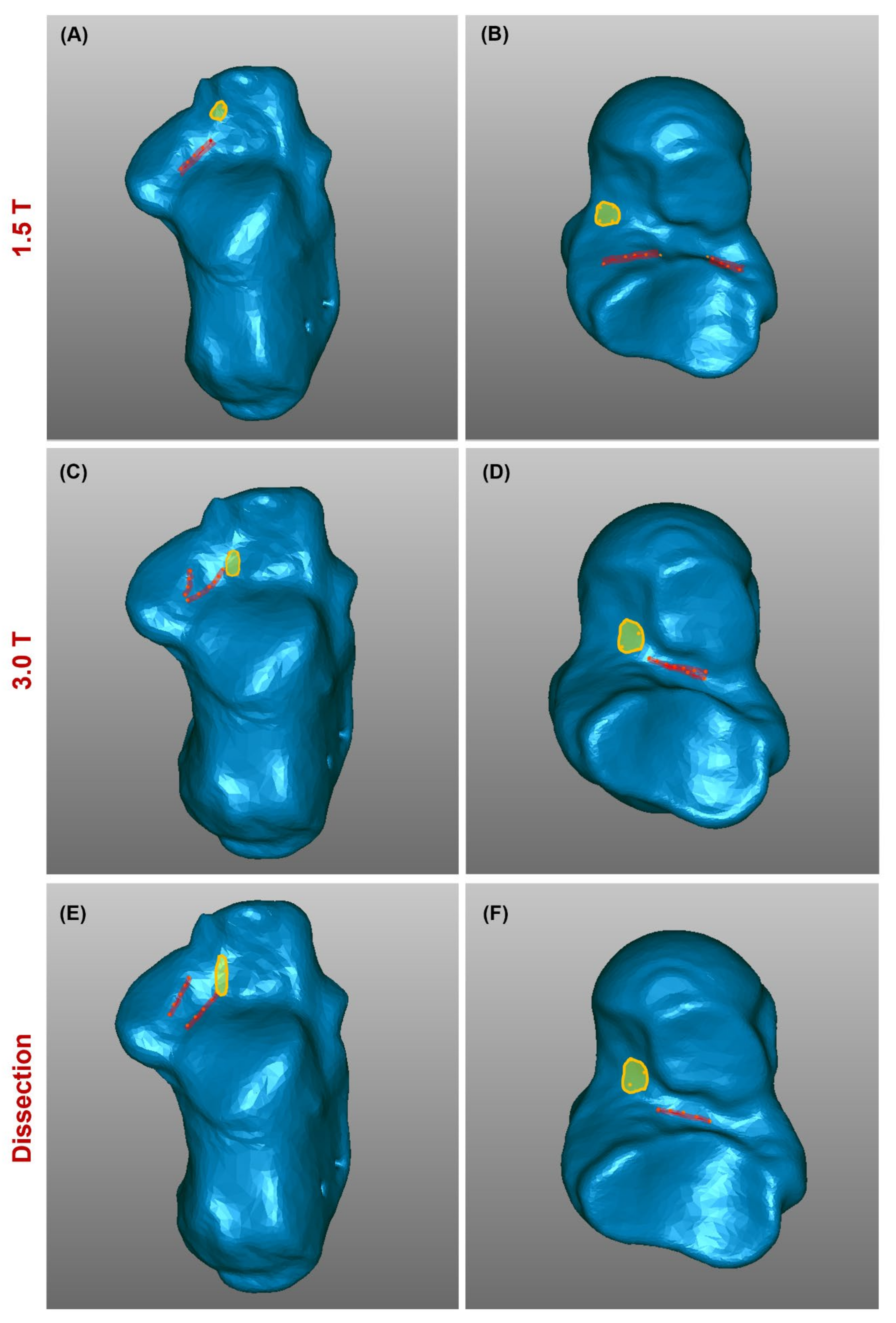
2.2. Identification of 1.5 T MRI-Based Ligament Attachments

2D and 3D sequences were acquired with 1.5 T MRI (SIGNA EXCITE HDxt, GE Healthcare, Chicago, IL, USA). In detail, 3D Cube acquisition was executed using a Quad Knee coil with 0.5 mm slice thickness and 0.6 × 0.6 × 0.5 mm voxel size; 2D Fat-Sat axial, coronal and sagittal were also acquired with 3.3 mm slice thickness and 0.3 × 0.3 × 3.3 mm voxel size.

The ligament attachment areas were segmented starting from the 3D sequence. However, due to the low overall image quality resulting from this scan, morphological reconstruction was obtained by combining relevant information with that derived from the 2D sequences. The obtained ligament attachment areas were then compared to those present in the original model [12]. When differences in attachment sites were observed, they were transferred to the dynamic model to replace the original ones.

2.3. Identification of 3.0 T MRI-Based Ligament Attachments

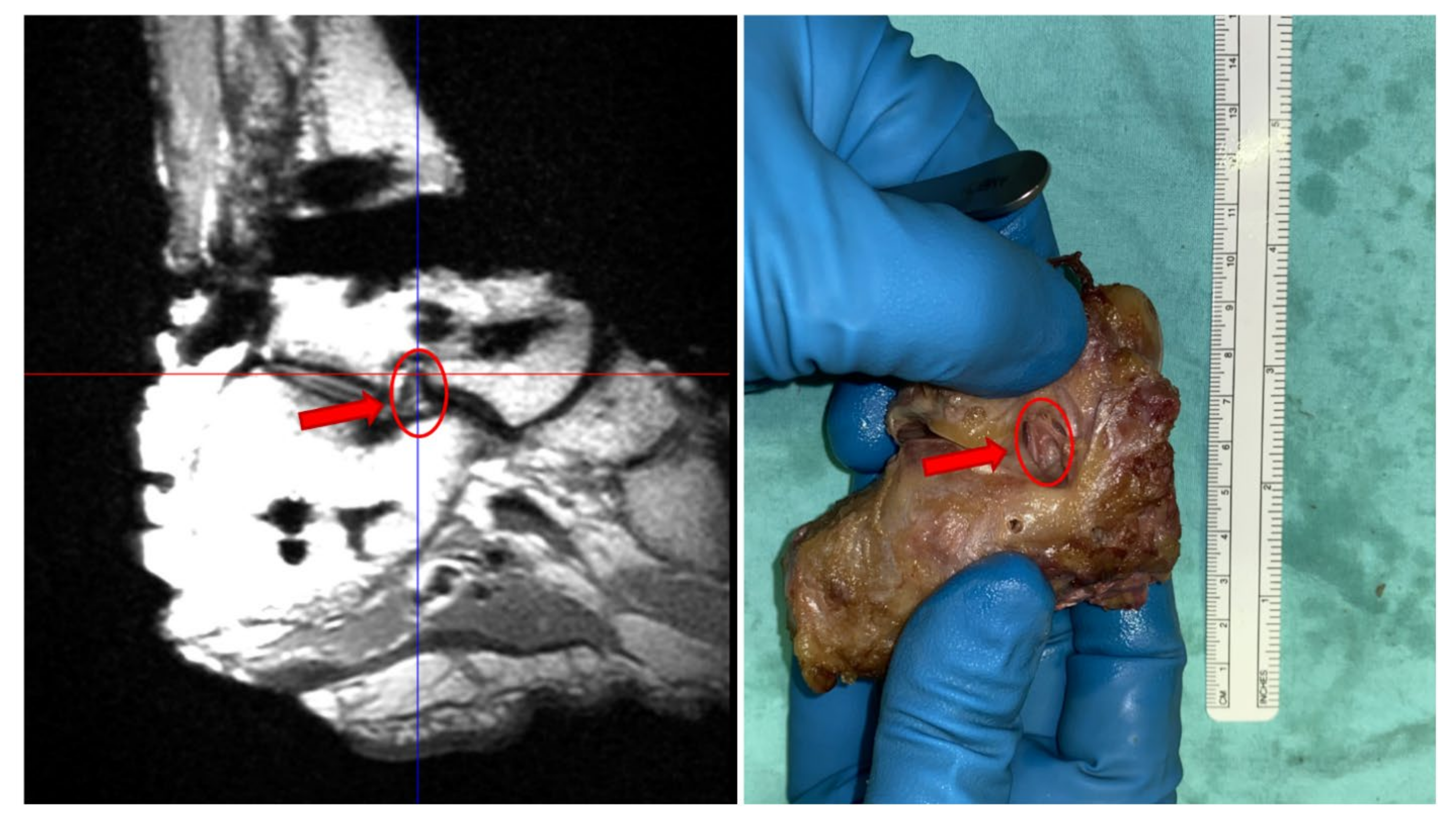
2D and 3D sequences were acquired with 3.0 T MRI (MR750W GEM ENAB, GE Healthcare, Chicago, IL, USA). In detail, 3D Cube acquisition was executed using a 16-ch gem flex medium coil, with 0.4 mm slice thickness and 0.4 × 0.4 × 0.4 mm voxel size; 2D Fat-Sat axial, coronal, and sagittal were acquired with 3.0 mm slice thickness and 0.5 × 0.5 × 3.0 mm voxel size.

The ligament attachment areas were segmented from the 3D Cube sequence which, in this case, provided high quality images, although 2D sequences were always analysed for completeness. Thanks to the overall better resolution of the 3D Cube of 3.0 T MRI scan when compared to the corresponding from 1.5 T MRI scan, several reslicing were here performed to best identify the regions of origin and insertion of the different ligaments. The reslicing process maintained full resolution since no deterioration resulted from the adopted process. The obtained ligament attachment areas were then compared to those present in the original model [12]. When differences in attachment sites were observed, they were transferred to the dynamic model to replace the original ones.

3. Dissection

The same specimen, a below-knee amputation from a fresh frozen cadaver, was dissected to provide direct access and visualization of the morphology of the ligament attachment sites, and these were used as a reference for the image-based assessments. All soft tissues were removed, and the ligaments of interest were exposed. Each ligament was photographed and marked with a surgical marking pen. The ligament attachment sites of data were compared to those present in the original model [12]. When differences in attachment sites were observed, they were transferred to the dynamic model to replace the original ones.

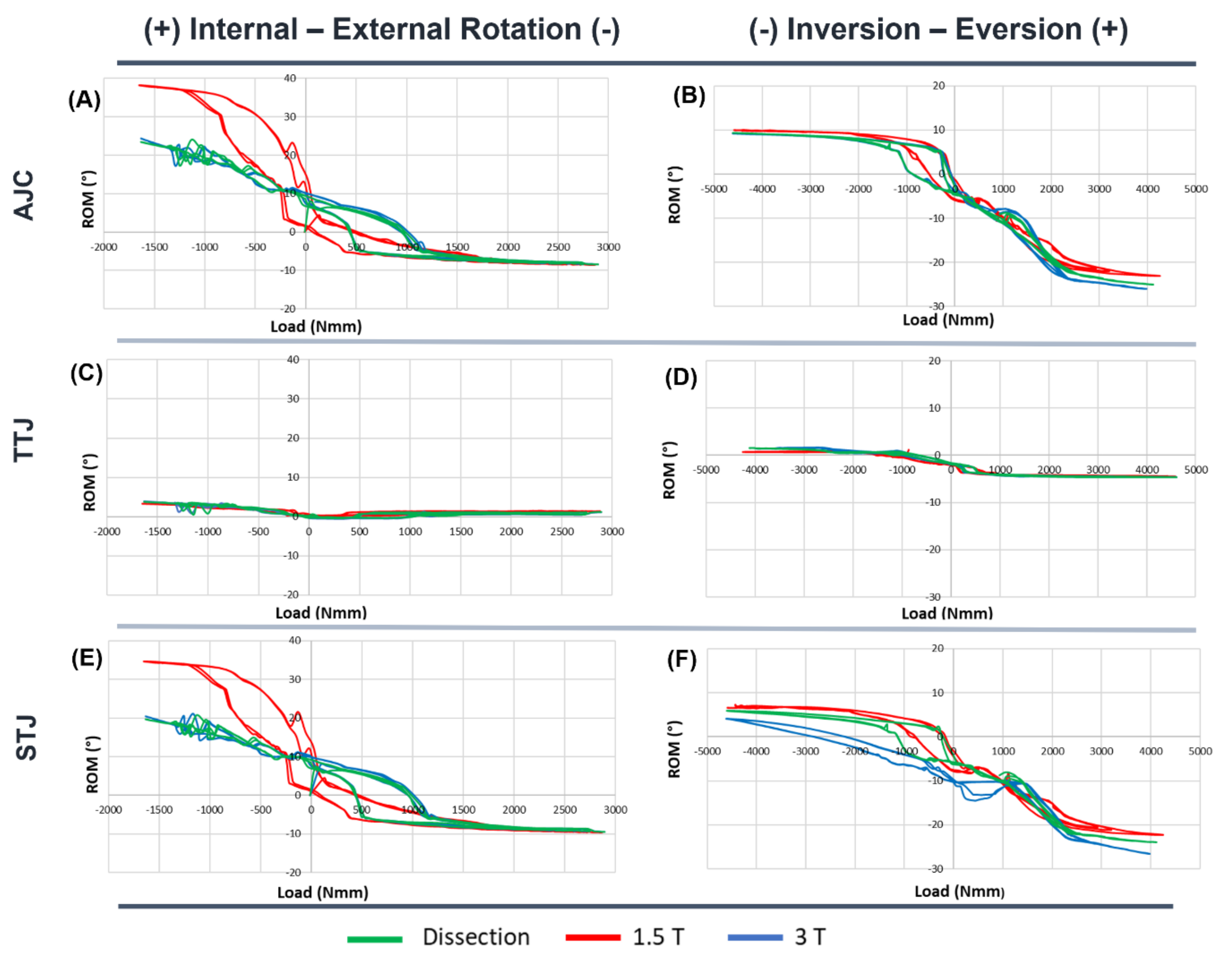
Model Simulations with Updated Mapping

Three different models were derived from the original model [12] for this specific specimen used in this study. Two models were based on MRI (1.5 T and 3.0 T) and one on the dissection-based observations. The only difference between each of these models and the original one was in the attachment sites of some of the ligaments, but they used loading and boundary conditions identical to those described earlier [20]. Simulations were performed (MSC ADAMS^TM, Newport Beach, CA, USA) by imposing 100 N axial compression and applying loading/unloading cycles in the frontal plane and axial plane. Load–displacement properties were obtained in inversion–eversion and internal–external rotation for the tibiotalar joint (TTJ), the subtalar joint (STJ), and the ankle joint complex (AJC) for each of the three models.

4. Results

The ligaments attachment sites obtained from the 3.0 T MRI were better visualized than those from 1.5 T MRI and their locations were more consistent with those obtained from direct observations. All these three definition schemes provided similar data on the origin and insertion sites for the ankle complex ligaments, except for those of the subtalar joint, particularly for the ITCL. In the 1.5 T MRI, the ITCL consisted of two branches with a common insertion on the calcaneus (Figure 1A), which split in two distinguished origins on the lower surface of the talus (Figure 1B), one more lateral and the other more medial. In the 3.0 T MRI, the common origin was on the talus (Figure 1D) and then the two branches divided into a more anterior insertion area and a more posterior one on the lateral part of the lower surface of the calcaneus (Figure 1C). Overall, ligament attachment sites from the 3.0 T MRI were consistent with the direct observations from dissection (compare Figure 1E,F and Figure 2 left and right).

In Figure 3, the load–displacement curves for the TTJ, STJ, and AJC in internal–external rotation and inversion–eversion were obtained from the three different schemes. For the AJC, similar load–displacement patterns were observed in the frontal plane (Figure 3B). In the transverse plane (Figure 3A), 1.5 T MRI model produced a different pattern when compared to the other two, reaching about 40° of internal rotation as compared to only 25°.

For TTJ (Figure 3C,D) the three schemes resulted in similar load–displacement patterns in both the frontal and axial plane.

The differences in the load–displacement properties between the three different schemes for the STJ (Figure 3E,F) are similar to those for the AJC, i.e., with 3.0 T MRI generally replicating results from the dissection map.

5. Discussion

The attachment areas of ankle and subtalar ligaments were identified using 1.5 T and 3.0 T MRI systems via both 2D and 3D sequences, and also via direct observations used as a reference. After relevant redistribution of the ligament fibres, a dynamic analysis of an ankle complex model showed load–displacement curves based on the 3.0 T MRI observations more consistent with those curves based on direct observations of the specimen.

A number of papers in radiologic anatomy have addressed MRI imaging for ankle complex ligaments [40,41,42,43]. However, these have not dealt with careful definition of origin and insertion areas of the ligaments, and this is particularly true for the subtalar ligaments. Additionally, not a single paper has compared geometrical and morphological features of these ligaments with corresponding direct observations. Also very limited is the analysis of the effects of resulting ligament mapping on dynamic computer models of the ankle joint complex. A recent paper from these authors has addressed medical imaging of the ankle complex by different modalities [44], but with a focus on the articular cartilage.

The comparison of the ligament attachment sites obtained using the two MRI modalities with the direct observations demonstrated the superiority of the 3.0 T MRI over the 1.5 T MRI in imaging ligaments and identifying their regions of origin and insertion on bones. The main reason for these differences was that the 3D Cube sequence in 3.0 T MRI allows for a clearer visualization and revisualization of the ligaments and their attachment areas without losing resolution. In addition, 3.0 T MRI provides twice the signal-to-noise ratio compared to 1.5 T MRI, resulting in better image quality and higher spatial resolution [35].

Visualization through imaging of the subtalar ligament morphology is very difficult [23,40]. This study demonstrated that this difficulty may be overcome by more advanced imaging modalities and may offer a solution for accurate diagnosis of subtalar ligament injuries [8,24]. Furthermore, this study demonstrated that visualizing the subtalar ligaments from different orientations without loss of resolution provides an important imaging advantage over non-cubic sequences where high resolution is only available in one direction.

The 3.0 T MRI-based dynamic model produced load–displacement behaviour similar to that resulting from the model based on direct observations of the ligaments attachment sites. The 1.5 T MRI-based model, on the other hand, produced different results. This demonstrates the importance of using higher resolution 3D Cube sequence, as by 3.0 T MRI, in developing accurate models of the ankle complex and its ligamentous support.

This study is not without limitations. The study relied on one single specimen so that inter-subject variability was not considered. In addition, direct observation, even from very careful anatomical dissections by experienced anatomists and surgeons, is difficult and subject to controversies due to the complex structure of these ligaments and their hard-to-access location. This also applies to identification by radiologists in image-based observations. In addition, no inter-observer assessment was included. The present relevant findings can be certainly strengthened in the future with other specimens, other MRI devices, and other ligament mapping definitions.

6. Conclusions

The present study offers an enhancement for subject-specification of a previously validated 3D dynamic model of the ankle complex [12,17] through MRI-based mappings of the ligaments from a single representative specimen. The results obtained from the two MRI systems and the anatomical dissection of the same specimen demonstrated how essential the identification of ligaments origin and insertion sites is for subject-specific modelling of the ankle complex. In particular, the better quality of the state-of-the-art 3.0 T MRI images, with respect to traditional 1.5 T MRI, resulted in definitions of these attachment sites closer to the direct observations, and in more similar load–displacement curves from the computer model.

References

1. Leardini, A.; O’Connor, J.J.; Catani, F.; Giannini, S. The role of the passive structures in the mobility and stability of the human ankle joint: A literature review. Foot Ankle Int. 2000, 21, 602–615. [Google Scholar] [CrossRef] [PubMed]
2. Stagni, R.; Leardini, A.; O’Connor, J.J.; Giannini, S. Role of passive structures in the mobility and stability of the human subtalar joint: A literature review. Foot Ankle Int. 2003, 24, 402–409. [Google Scholar] [CrossRef] [PubMed]
3. Petersen, W.; Rembitzki, I.V.; Koppenburg, A.G.; Ellermann, A.; Liebau, C.; Bruggemann, G.P.; Best, R. Treatment of acute ankle ligament injuries: A systematic review. Arch. Orthop. Trauma. Surg. 2013, 133, 1129–1141. [Google Scholar] [CrossRef] [PubMed] [Green Version]
4. Van den Bekerom, M.P.; Kerkhoffs, G.M.; McCollum, G.A.; Calder, J.D.; van Dijk, C.N. Management of acute lateral ankle ligament injury in the athlete. Knee Surg. Sports Traumatol. Arthrosc. Off. J. ESSKA 2013, 21, 1390–1395. [Google Scholar] [CrossRef]
5. Guillo, S.; Bauer, T.; Lee, J.W.; Takao, M.; Kong, S.W.; Stone, J.W.; Mangone, P.G.; Molloy, A.; Perera, A.; Pearce, C.J.; et al. Consensus in chronic ankle instability: Aetiology, assessment, surgical indications and place for arthroscopy. Orthop. Traumatol. Surg. Res. 2013, 99, S411–S419. [Google Scholar] [CrossRef] [Green Version]
6. Michels, F.; Pereira, H.; Calder, J.; Matricali, G.; Glazebrook, M.; Guillo, S.; Karlsson, J.; Group, E.-A.A.I.; Acevedo, J.; Batista, J.; et al. Searching for consensus in the approach to patients with chronic lateral ankle instability: Ask the expert. Knee Surg. Sports Traumatol. Arthrosc. Off. J. ESSKA 2018, 26, 2095–2102. [Google Scholar] [CrossRef]
7. Yamaguchi, R.; Nimura, A.; Amaha, K.; Yamaguchi, K.; Segawa, Y.; Okawa, A.; Akita, K. Anatomy of the Tarsal Canal and Sinus in Relation to the Subtalar Joint Capsule. Foot Ankle Int. 2018, 39, 1360–1369. [Google Scholar] [CrossRef]
8. Kim, T.H.; Moon, S.G.; Jung, H.G.; Kim, N.R. Subtalar instability: Imaging features of subtalar ligaments on 3D isotropic ankle MRI. BMC Musculoskelet. Disord. 2017, 18, 475. [Google Scholar] [CrossRef] [Green Version]
9. Leardini, A.; O’Connor, J.J.; Giannini, S. Biomechanics of the natural, arthritic, and replaced human ankle joint. J. Foot Ankle Res. 2014, 7, 8. [Google Scholar] [CrossRef] [Green Version]
10. Nie, B.; Panzer, M.B.; Mane, A.; Mait, A.R.; Donlon, J.P.; Forman, J.L.; Kent, R.W. Determination of the in situ mechanical behavior of ankle ligaments. J. Mech. Behav. Biomed. Mater. 2017, 65, 502–512. [Google Scholar] [CrossRef]
11. Iaquinto, J.M.; Wayne, J.S. Computational model of the lower leg and foot/ankle complex: Application to arch stability. J. Biomech. Eng. 2010, 132, 021009. [Google Scholar] [CrossRef] [PubMed]
12. Imhauser, C.W.; Siegler, S.; Udupa, J.K.; Toy, J.R. Subject-specific models of the hindfoot reveal a relationship between morphology and passive mechanical properties. J. Biomech. 2008, 41, 1341–1349. [Google Scholar] [CrossRef] [PubMed] [Green Version]
13. Leardini, A.; O’Connor, J.J.; Catani, F.; Giannini, S. A geometric model of the human ankle joint. J. Biomech. 1999, 32, 585–591. [Google Scholar] [CrossRef]
14. Forlani, M.; Sancisi, N.; Parenti-Castelli, V. A three-dimensional ankle kinetostatic model to simulate loaded and unloaded joint motion. J. Biomech. Eng. 2015, 137, 061005. [Google Scholar] [CrossRef] [PubMed]
15. Liacouras, P.C.; Wayne, J.S. Computational modeling to predict mechanical function of joints: Application to the lower leg with simulation of two cadaver studies. J. Biomech. Eng. 2007, 129, 811–817. [Google Scholar] [CrossRef]
16. Purevsuren, T.; Kim, K.; Batbaatar, M.; Lee, S.; Kim, Y.H. Influence of ankle joint plantarflexion and dorsiflexion on lateral ankle sprain: A computational study. Proc. Inst. Mech. Eng. Part H 2018, 232, 458–467. [Google Scholar] [CrossRef]
17. Palazzi, E.; Siegler, S.; Balakrishnan, V.; Leardini, A.; Caravaggi, P.; Belvedere, C. Estimating the stabilizing function of ankle and subtalar ligaments via a morphology-specific three-dimensional dynamic model. J. Biomech. 2020, 98, 109421. [Google Scholar] [CrossRef]
18. Li, J.; Wei, Y.; Wei, M. Finite Element Analysis of the Effect of Talar Osteochondral Defects of Different Depths on Ankle Joint Stability. Med. Sci. Monit. 2020, 26, e921823. [Google Scholar] [CrossRef]
19. Haraguchi, N.; Armiger, R.S.; Myerson, M.S.; Campbell, J.T.; Chao, E.Y. Prediction of three-dimensional contact stress and ligament tension in the ankle during stance determined from computational modeling. Foot Ankle Int. 2009, 30, 177–185. [Google Scholar] [CrossRef]
20. Belvedere, C.; Siegler, S.; Ensini, A.; Toy, J.; Caravaggi, P.; Namani, R.; Giannini, G.; Durante, S.; Leardini, A. Experimental evaluation of a new morphological approximation of the articular surfaces of the ankle joint. J. Biomech. 2017, 53, 97–104. [Google Scholar] [CrossRef]
21. Golano, P.; Vega, J.; de Leeuw, P.A.; Malagelada, F.; Manzanares, M.C.; Gotzens, V.; van Dijk, C.N. Anatomy of the ankle ligaments: A pictorial essay. Knee Surg. Sports Traumatol. Arthrosc. Off. J. ESSKA 2010, 18, 557–569. [Google Scholar] [CrossRef] [PubMed] [Green Version]
22. Anand Prakash, A. Anatomy of Ankle Syndesmotic Ligaments: A Systematic Review of Cadaveric Studies. Foot Ankle Spec. 2020, 13, 341–350. [Google Scholar] [CrossRef] [PubMed]
23. Michels, F.; Matricali, G.; Vereecke, E.; Dewilde, M.; Vanrietvelde, F.; Stockmans, F. The intrinsic subtalar ligaments have a consistent presence, location and morphology. Foot Ankle Surg. 2021, 27, 101–109. [Google Scholar] [CrossRef] [PubMed]
24. Poonja, A.J.; Hirano, M.; Khakimov, D.; Ojumah, N.; Tubbs, R.S.; Loukas, M.; Kozlowski, P.B.; Khan, K.H.; DiLandro, A.C.; D’Antoni, A.V. Anatomical Study of the Cervical and Interosseous Talocalcaneal Ligaments of the Foot with Surgical Relevance. Cureus 2017, 9, e1382. [Google Scholar] [CrossRef] [Green Version]
25. Sconfienza, L.M.; Orlandi, D.; Lacelli, F.; Serafini, G.; Silvestri, E. Dynamic high-resolution US of ankle and midfoot ligaments: Normal anatomic structure and imaging technique. Radiographics 2015, 35, 164–178. [Google Scholar] [CrossRef]
26. Ngai, S.S.; Tafur, M.; Chang, E.Y.; Chung, C.B. Magnetic Resonance Imaging of Ankle Ligaments. Can. Assoc. Radiol. J. 2016, 67, 60–68. [Google Scholar] [CrossRef] [Green Version]
27. Chen, E.T.; Borg-Stein, J.; McInnis, K.C. Ankle Sprains: Evaluation, Rehabilitation, and Prevention. Curr. Sports Med. Rep. 2019, 18, 217–223. [Google Scholar] [CrossRef]
28. Van Dyck, P.; Kenis, C.; Vanhoenacker, F.M.; Lambrecht, V.; Wouters, K.; Gielen, J.L.; Dossche, L.; Parizel, P.M. Comparison of 1.5-and 3-T MR imaging for evaluating the articular cartilage of the knee. Knee Surg. Sports Traumatol. Arthrosc. Off. J. ESSKA 2014, 22, 1376–1384. [Google Scholar] [CrossRef]
29. Van Dyck, P.; Vanhoenacker, F.M.; Lambrecht, V.; Wouters, K.; Gielen, J.L.; Dossche, L.; Parizel, P.M. Prospective comparison of 1.5 and 3.0-T MRI for evaluating the knee menisci and ACL. J. Bone Jt. Surg. 2013, 95, 916–924. [Google Scholar] [CrossRef]
30. Nouri, N.; Bouaziz, M.C.; Riahi, H.; Mechri, M.; Kherfani, A.; Ouertatani, M.; Ladeb, M.F. Traumatic Meniscus and Cruciate Ligament Tears in Young Patients: A Comparison of 3T Versus 1.5T MRI. J. Belg. Soc. Radiol. 2017, 101, 14. [Google Scholar] [CrossRef] [Green Version]
31. Grossman, J.W.; De Smet, A.A.; Shinki, K. Comparison of the accuracy rates of 3-T and 1.5-T MRI of the knee in the diagnosis of meniscal tear. AJR Am. J. Roentgenol. 2009, 193, 509–514. [Google Scholar] [CrossRef] [PubMed]
32. Barr, C.; Bauer, J.S.; Malfair, D.; Ma, B.; Henning, T.D.; Steinbach, L.; Link, T.M. MR imaging of the ankle at 3 Tesla and 1.5 Tesla: Protocol optimization and application to cartilage, ligament and tendon pathology in cadaver specimens. Eur. Radiol. 2007, 17, 1518–1528. [Google Scholar] [CrossRef] [PubMed]
33. Oehler, N.; Ruby, J.K.; Strahl, A.; Maas, R.; Ruether, W.; Niemeier, A. Hip abductor tendon pathology visualized by 1.5 versus 3. 0 Tesla MRIs. Arch. Orthop. Trauma. Surg. 2020, 140, 145–153. [Google Scholar] [CrossRef] [PubMed]
34. Bauer, J.S.; Barr, C.; Henning, T.D.; Malfair, D.; Ma, C.B.; Steinbach, L.; Link, T.M. Magnetic resonance imaging of the ankle at 3.0 Tesla and 1.5 Tesla in human cadaver specimens with artificially created lesions of cartilage and ligaments. Investig. Radiol. 2008, 43, 604–611. [Google Scholar] [CrossRef]
35. Bauer, J.S.; Monetti, R.; Krug, R.; Matsuura, M.; Mueller, D.; Eckstein, F.; Rummeny, E.J.; Lochmueller, E.M.; Raeth, C.W.; Link, T.M. Advances of 3T MR imaging in visualizing trabecular bone structure of the calcaneus are partially SNR-independent: Analysis using simulated noise in relation to micro-CT, 1.5T MRI, and biomechanical strength. J. Magn. Reson. Imaging 2009, 29, 132–140. [Google Scholar] [CrossRef]
36. Neri, E.; Caramella, D.; Bartolozzi, C. Image Processing in Radiology: Current Applications; Springer: Berlin, Germany; New York, NY, USA, 2008; p. x, 434p. [Google Scholar]
37. Stevens, K.J.; Busse, R.F.; Han, E.; Brau, A.C.; Beatty, P.J.; Beaulieu, C.F.; Gold, G.E. Ankle: Isotropic MR imaging with 3D-FSE-cube--initial experience in healthy volunteers. Radiology 2008, 249, 1026–1033. [Google Scholar] [CrossRef] [Green Version]
38. Siegler, S.; Block, J.; Schneck, C.D. The mechanical characteristics of the collateral ligaments of the human ankle joint. Foot Ankle 1988, 8, 234–242. [Google Scholar] [CrossRef]
39. Funk, J.R.; Hall, G.W.; Crandall, J.R.; Pilkey, W.D. Linear and quasi-linear viscoelastic characterization of ankle ligaments. J. Biomech. Eng. 2000, 122, 15–22. [Google Scholar] [CrossRef]
40. Lopez-Ben, R. Imaging of the subtalar joint. Foot Ankle Clin. 2015, 20, 223–241. [Google Scholar] [CrossRef]
41. Sormaala, M.J.; Ruohola, J.P.; Mattila, V.M.; Koskinen, S.K.; Pihlajamaki, H.K. Comparison of 1.5T and 3T MRI scanners in evaluation of acute bone stress in the foot. BMC Musculoskelet. Disord. 2011, 12, 128. [Google Scholar] [CrossRef] [Green Version]
42. Cledera, T.H.C.; Flores, D.V. Magnetic Resonance Imaging of Ankle Ligaments. Contemp. Diagn. Radiol. 2021, 44, 1–7. [Google Scholar] [CrossRef]
43. Fritz, B.; Fritz, J.; Sutter, R. 3D MRI of the Ankle: A Concise State-of-the-Art Review. Semin. Musculoskelet. Radiol. 2021, 25, 514–526. [Google Scholar] [CrossRef] [PubMed]
44. Durastanti, G.; Leardini, A.; Siegler, S.; Durante, S.; Bazzocchi, A.; Belvedere, C. Comparison of cartilage and bone morphological models of the ankle joint derived from different medical imaging technologies. Quant. Imaging Med. Surg. 2019, 9, 1368–1382. [Google Scholar] [CrossRef] [PubMed]
Figure 1. Maps of the subtalar ligaments from 1.5 T MRI (A,B), 3.0 T MRI (C,D), and from dissection (E,F): CL (yellow), ITCL (red). Origin areas on the bottom of the talus bone (B,D,F) and insertion areas on the top of the calcaneus bone (A,C,E).
Applsci 12 05087 g001
Figure 2. ITCL from 3.0 T MRI (left) and from direct observation (right).
Applsci 12 05087 g002
Figure 3. Superimposition of the load–displacement curves resulting from the three mappings of the ligament attachment sites obtained via 1.5 T (red curves), 3.0 T (blue curves), and direct observation from the dissection of the specimen (green curves). Curves associated to Internal–External Rotation (A,C,E) and Inversion–Eversion (B,D,F) are reported for the AJC (A,B), TTJ (C,D), and STJ (E,F).
Applsci 12 05087 g003
Publisher’s Note: MDPI stays neutral with regard to jurisdictional claims in published maps and institutional affiliations.