Nonlinear Dynamics of an Elastic Stop System and Its Application in a Rotor System

Abstract

Impact dampers or vibration systems with gaps are common in engineering applications, and the impact effects introduced by the gaps make such systems strongly nonlinear. In this paper, a model with an elastic stop is established, considering the stiffness and damping characteristics of the stop, which is a novel kind of impact damper and can be applied in a rotor system. The amplitude–frequency and phase–frequency response of the system at different gaps are obtained by the harmonic balance method with the alternating frequency–time scheme (HBM-AFT). The stability of the periodic solution is analyzed by the Floquet theory, and the time history and frequency spectra of the unstable point are analyzed by the numerical integration method. In the results, there can be more than one steady-state response at unstable points for a given excitation frequency, and the jump phenomenon occurs. The elastic stop is effective in the vibration amplitude suppression if its stiffness has been designed properly. This study provides an insight into the dynamic responses and its applications of the system with gaps, which is guidance for the analysis of pedestal looseness faults and vibration suppress methods.

1. Introduction

Impact dampers or vibration systems with gaps are common in engineering applications, and the impact effects introduced by the gaps make such systems strongly nonlinear. These systems are generally simplified to spring–mass systems with displacement limits, and the limiting effects are expressed using piecewise linear functions. Thompson et al. [1,2] carried out numerical simulations of a single-degree-of-freedom (Dof) model with piecewise linear stiffness properties, showing a series of sub-harmonic frequency components in the response, finding that period-doubling bifurcation is one of the causes of the chaotic motion.

Shaw et al. [3,4] developed a one-dimensional impact damper model. They derived its response using analytical methods to theoretically verify and analyze the mechanism of the harmonic frequency components in the response and the bifurcation phenomenon. Moreover, this paper introduced the early studies of the single-Dof model with impact problems. In the subsequent investigations, most scholars used this model as the basis and mainly explored the analytical methods and the influence of system parameters on the free vibration and forced response. Hindmarsh et al. [5] established the one-dimensional bilinear stiffness model, investigated the stability of the periodic motion and the bifurcation characteristics using analytical methods, and explored the relationship between the stability and bifurcation phenomenon. Peterka [6] compared the effects of a rigid and elastic stop on the dynamics of the system with impact effects and then summarized the similarities and differences between the response of elastic and rigid stops. Bapat [7] derived an exact solution for the response of a one-dimensional system with a one-sided stop. The governing equations are established by bilinear stiffness and bilinear damping.

In the study of single-Dof models, the nonsmooth properties of the stop can be expressed in various approximate functional forms such as piecewise nonlinear functions or Taylor expansions, in addition to being characterized by piecewise linear functions. Kong and Wen [8] studied the guideway motion by reducing it to a one-dimensional dynamical system with piecewise nonlinear stiffness and used the incremental harmonic balance method to obtain the amplitude–frequency curves, where a significant hardening spring phenomenon can be seen in the results. Wang et al. [9] proposed an improved incremental harmonic balance method and used the proposed approach to analyze the dynamic response of a one-dimensional system containing piecewise nonlinear stiffness.

The studies above analyzed the dynamical characteristics of one-dimensional nonsmooth systems in terms of frequency spectra, stability, bifurcation phenomena, chaotic motion, etc. Many scholars tried to introduce this nonsmooth model into multi-Dof systems and studied their effects on the dynamical response. Aidanpaa and Gupta [10] established a two-Dof nonsmooth model, in which, due to the assumption of absolute rigid stop, there is a significant cut-off phenomenon in the response. Natsiavas [11] introduced nonsmooth functions to general multi-Dof systems, analyzed a model with two-Dof, and found Hopf and period doubling bifurcations, as well as the 2:1 and 3:1 internal resonance phenomena. Luo and Xie [12] investigated the Hopf bifurcation behavior of a two-Dof system with impact effects and verified the analytical results through numerical simulations. Valente et al. [13] studied the impact of a fixed stop on the two-Dof system based on a piecewise linear model. Pascal [14,15] investigated the effect of the stiffness of the stop on the dynamic response of the two-Dof system based on analytical approaches and compared the characteristics of the time-domain response of the system under rigid and elastic stops.

In addition to discrete models, the above analytical methods and conclusions are generally applicable to the response analysis of a continuous model with nonsmooth constraints based on piecewise linear functions. For example, Brake [16] introduced nonsmooth constraints with piecewise linear stiffness into a continuous beam model. It analyzed the effect of the stop on the frequency domain components and the stability of the periodic solution. Studies of the piecewise linear or nonlinear systems can explain and analyze the dynamical behavior of structural systems containing stops, which is essential guidance for engineering applications. In addition, the analysis of such nonlinear systems can also be applied to develop vibration suppression or control methods for general structural systems. For example, a stop was applied to develop a nonlinear dynamic absorber for vibration suppression of single-Dof systems [17].

Dynamic responses of the system with impact effects are strongly nonlinear, and a very general method to solve them does not exist. As for the case of the system with piecewise linear functions, the dynamic behavior can be usually obtained by using the experimental rig and semi-analytical methods. Ing et al. [18] studied the bifurcation diagrams of an impact oscillator with a one-side elastic constraint based on the mapping theory, and they performed relevant experiments to verify the results. Bureau et al. [19] investigated the stability and bifurcation of an impact oscillator experimentally. Tan et al. [20] investigated the vibration behavior of a piping system with delimiters to passively suppress the vibrations by using experimental rigs. Although the results of experiments are most persuasive, carrying out experiments may be expensive and difficult. Therefore, semi-analytical methods like the harmonic balance method (HBM) with alternating frequency/time method (AFT) can be applied more easily. Yoon et al. [21] studied the gear system with piecewise-type nonlinearities using the HBM. Pei et al. [22] computed the periodic orbits of a piecewise linear oscillator by HBM and AFT. Moreover, the perturbation technique is also a highly efficient method to investigate nonlinear systems. Amer et al. [23] promoted a novel nonlinear system and gave essential insights into a new vibrating dynamical motion by the perturbation technique of multiple scales. Abdelhfeez et al. [24] explored interesting behaviors of a novel dynamical system with nonlinearities caused by the triple pendulum using the multiple scales method.

Mechanical systems with piecewise-type nonlinearities are common in machinery. For example, pedestal looseness of a rotor–support system is one of the common faults that occur in rotating machinery. It is usually caused by the poor quality of assembly or long-term vibration. Goldman and Muszynska [25,26] simplified the pedestal looseness rotor as a single-Dof vibration system with bi-linear form stiffness and performed analytical, numerical, and experimental investigations on the dynamic behavior. Super-harmonic and sub-harmonic frequency components were found, which implied synchronous and sub-synchronous fractional motions. Chu et al. [27,28] studied the periodical motions and stabilities of a simplified pedestal looseness rotor and verified sub-synchronous motions with an experimental rig. Ma et al. [29] established a pedestal looseness model by combining FEM and piecewise linear form and studied the influences of the gap size on the response. Lu et al. [30] studied a multi-disk rotor with the pedestal looseness fault based on HBM. Chen et al. [31,32] investigated the super-harmonic frequency components by a numerical method and verified by experiments. Although the above papers provide an important insight into the pedestal looseness faults caused by loosed bolts between the bearing house and pedestal for most rotating machinery, few studies focused on the other kind of pedestal looseness fault caused by the gap between the bearing outer ring and the bearing house. Chen et al. [33,34] considered the fitting clearance between a bearing and its bearing house, and performed numerical and experimental investigations on the dynamic response.

As far as we know, although systems with piecewise type nonlinearities have been investigated from many aspects, the mass of the elastic stop has been usually ignored in the existing studies. Therefore, in this paper, based on the piecewise linear model of a single-Dof system, a novel two-Dof model with an elastic stop considering the stop’s mass, stiffness, and damping is established. The effect of impact on the dynamics of the system is studied in detail, which is important for explaining the dynamical behavior or the design of dynamic characteristics of such systems. In addition, based on the results of the two-Dof model, the characteristics of a new pedestal loosening rotor with an overhanging disk and three supports have been investigated, and the feasibility of vibration suppression of a flexible rotor using an elastic stop has been discussed.

2. Model and Solving Method

2.1. Model

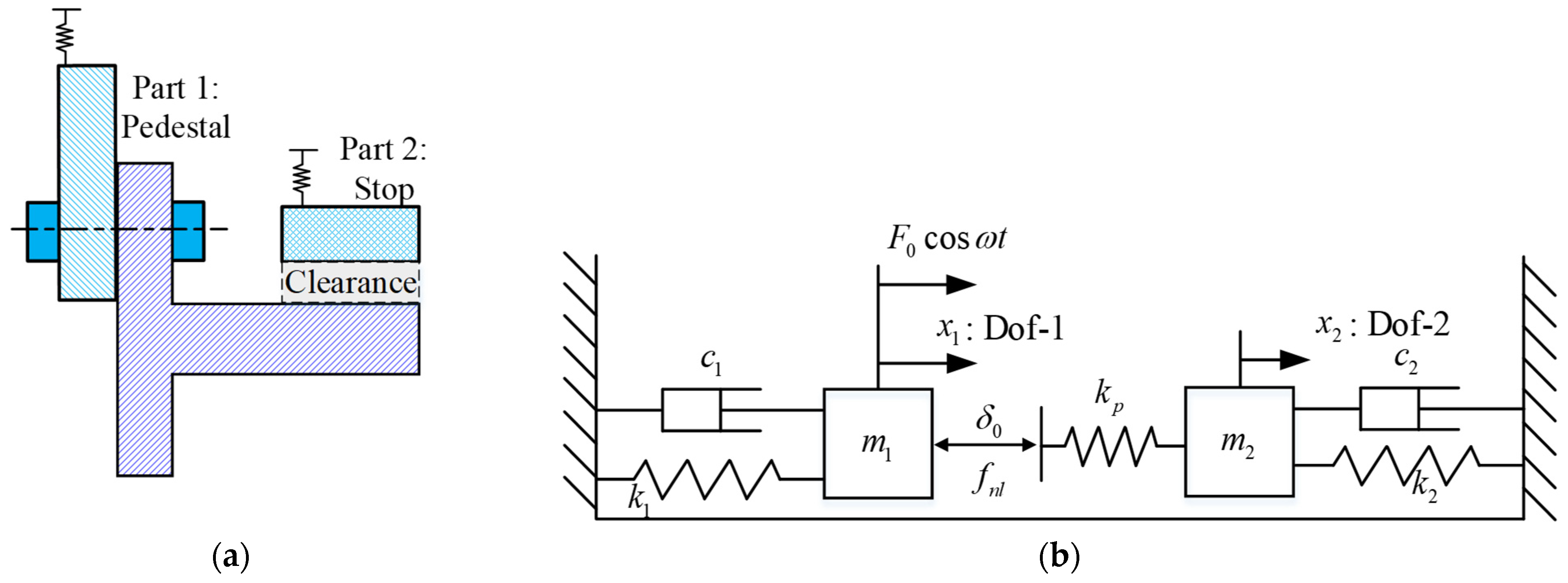
In this paper, a two-Dof model with an elastic stop is established, as shown in Figure 1, and the influence of the stop on the dynamic characteristics of the system is investigated.

A typical system with gaps is a pedestal with a stop in a rotating mechanical system, shown in Figure 1a. In general, its stiffness and damping characteristics caused by intermittent contact can be characterized by a piecewise linear function, and this paper establishes a dynamic model as shown in Figure 1b.

The governing equations can be derived by Appendix A and are shown as follows:

$$\left[\begin{array}{cc}{m}_1& \\ & m_2\end{array}\right]\left\{\begin{array}{c}{\ddot{x}}_1\\ {\ddot{x}}_2\end{array}\right\}+\left[\begin{array}{cc}{c}_1& \\ & c_2\end{array}\right]\left\{\begin{array}{c}{\dot{x}}_1\\ {\dot{x}}_2\end{array}\right\}+\left[\begin{array}{cc}{k}_1& \\ & k_2\end{array}\right]\left\{\begin{array}{c}{x}_1\\ x_2\end{array}\right\}+f_{nl}=\left\{\begin{array}{c}{F}_0\cos \omega t\\ \end{array}\right\}$$

(1)

in which $m_1$ and $m_2$ are the mass of the two Dofs; $c_1$ and $c_2$ are the damping of the two Dofs; $k_1$ and $k_2$ are the stiffness of the two Dofs; $F_0$ is the amplitude of the external excitational force; and the stop is present by a piecewise stiffness so that the nonlinear force $f_{nl}$ is as follows:

$$\begin{array}{cc}{f}_{nl}& =k_p\left\{\begin{array}{c}{x}_1-x_2-{\delta }_0\\ -\left(x_1-x_2-{\delta }_0\right)\end{array}\right\}H\left(x_1-x_2-{\delta }_0\right)\hfill \\ & =k_{p}w\left(w^T\left\{\begin{array}{c}{x}_1\\ x_2\end{array}\right\}-{\delta }_0\right)H\left(w^T\left\{\begin{array}{c}{x}_1\\ x_2\end{array}\right\}-{\delta }_0\right)\hfill \\ & =k_{p}w{f}_c\left(w^T\left\{\begin{array}{c}{x}_1\\ x_2\end{array}\right\}-{\delta }_0\right)\hfill \end{array}$$

(2)

in which, the nonlinear force is denoted by the function $f_c(•)$ defined as follows,

$$f_c(•)=•H(•)$$

(3)

where $H(•)$ is the Heaviside function, namely, $H(•)=\{\begin{array}{c}1,•\ge 0\\ 0,•<0\end{array}$; $k_p$ is the penalty stiffness of the elastic stop, $w={\left[\begin{array}{cc}1& -1\end{array}\right]}^T$. A nominal restoring force $F^{*}$ is assumed to obtain dimensionless equations, and let

$${\Omega }^2=\frac{k_1}{m_1},\tau =\Omega t,\alpha =\frac{m_2}{m_1},\beta =\frac{c_2}{c_1},\gamma =\frac{k_2}{k_1},\widehat{\omega }=\frac{\omega }{\Omega },\zeta =\frac{c_1}{m_1\Omega },\widehat{F}=\frac{F_0}{F^{*}},\left[y\right]=\frac{k_1}{F^{*}}\left[x\right],\delta =\frac{k_1{\delta }_0}{F^{*}},\kappa =\frac{k_p}{k_1}.$$

(4)

In general, $F^{*}$ is usually assumed to be $k_1{\delta }_0$, which implies $\delta =1$ and $\left[y\right]=\left[x\right]/{\delta }_0$. Substitute Equation (4) into Equation (1); then, dimensionless governing equations are derived as follows:

$$\left[\begin{array}{cc}1& \\ & \alpha \end{array}\right]\left\{\begin{array}{c}{\ddot{y}}_1\\ {\ddot{y}}_2\end{array}\right\}+\left[\begin{array}{cc}\zeta & \\ & \beta \zeta \end{array}\right]\left\{\begin{array}{c}{\dot{y}}_1\\ {\dot{y}}_2\end{array}\right\}+\left[\begin{array}{cc}1& \\ & \gamma \end{array}\right]\left\{\begin{array}{c}{y}_1\\ y_2\end{array}\right\}+\kappa w{f}_c\left(w^T\left[y\right]-\delta \right)=\left\{\begin{array}{c}\widehat{F}\cos \widehat{\omega }\tau \\ \end{array}\right\}$$

(5)

In the subsequent analysis, the dimensionless parameters are $\alpha =1,\beta =1,\gamma =2$ and $\zeta =0.03,\widehat{F}=1$ if not specified.

2.2. Solving Method

One of the most popular methods for approximating the frequency response of a nonlinear system is known as the harmonic balance method (HBM) with the alternating frequency/time frame (AFT), which has been widely used in the nonlinear dynamic analysis. As for the above dynamic equations which are strongly nonlinear, steady-state periodic responses can be easily obtained by using the HBM-AFT methods. Thus, in this paper, the HBM-AFT method [35,36] and the shooting method are used to obtain their steady-state responses. The results are verified and supplemented by numerical integration methods. The critical process of the main techniques is given in the following.

The governing equations of a discrete system containing nonlinear forces can be expressed in the unified form:

$$M\ddot{x}\left(t\right)+D\dot{x}\left(t\right)+Kx\left(t\right)+g\left(x\left(t\right),\dot{x}\left(t\right)\right)=F_{ex}\left(t\right)$$

(6)

where, $x$,$\dot{x}$ and $\ddot{x}$ are the displacement, velocity, and acceleration vectors of the generalized degrees of freedom, respectively; $M$,$D$,$K$ and are the mass, damping, and stiffness matrices of the linear part; $g\left(x\left(t\right),\dot{x}\left(t\right)\right)$ denotes the nonlinear forces related to velocity and displacement, and $F_{ex}\left(t\right)$ is the external excitations.

When the external excitation of the system is a single sinusoidal excitation, the external excitation can be specified as

$$F_{ex}\left(t\right)=F_0\sin \nu \omega t$$

(7)

where $F_0$ is the vector of excitation magnitude, $\omega$ is the excitation frequency, and $\nu$ is the coefficient of the excitation frequency.

Based on the Fourier transform, the periodic solution of the response and the nonlinear forces are represented in the frequency domain by harmonic terms:

$$x\left(\theta \right)=A_0+{\displaystyle \sum _{k=1}^l\left(A_k\cos k\theta +B_k\sin k\theta \right)}$$

(8)

$$g\left(\theta \right)=P_0+{\displaystyle \sum _{k=1}^l\left(P_k\cos k\theta +Q_k\sin k\theta \right)}$$

(9)

where $l$ is the order truncated of harmonic terms, $\theta =\omega t$, $P_k$, $Q_k$, $A_k$ and $B_k$ are the constant vectors to be determined.

Since there is a nonlinear functional relationship between the nonlinear force and displacement in the time domain, there is a nonlinear functional relationship among $P_k$,$Q_k$, $A_k$ and $B_k$. However, for the generic nonlinear force, this inner relationship is not explicit in the frequency domain; thus, the time-frequency transformation technique is applied, and the principle is shown in Figure 2.

First, given the coefficients of a specific order harmonic term, define the number of time samples of the IFFT (IDFT) in one cycle as $N_{ts}$, then the value of the response of the nonlinear system at the $r^{st}$ discrete-time can be calculated as follows:

$${\tilde{x}}_r=real\left\{{\displaystyle \sum _{k=0}^l\left(A_k+j{B}_k\right)\left(\cos \frac{2\pi kr}{N_{st}}+j\sin \frac{2\pi kr}{N_{st}}\right)}\right\},r=0,1,2,\cdots ,N_{st}-1,j=\sqrt{-1}$$

(10)

Then, the nonlinear force is

$${\tilde{g}}_r=g\left({\tilde{x}}_r,{\dot{\tilde{x}}}_r\right)$$

(11)

Finally, the values of the nonlinear forces at all times are calculated, and the results of the nonlinear forces on the first-order harmonics in the frequency domain are obtained according to the DFT as

$${\tilde{g}}_k=\frac{\Psi }{N_{st}}{\displaystyle \sum _{r=0}^{N_{st}-1}{\tilde{g}}_r{e}^{j\left(-\frac{2\pi kr}{N_{st}}\right)}},\Psi =\{\begin{array}{cc}1,& k=0\\ 2,& k\ne 0\end{array}$$

(12)

Therefore, the implicit functional relationship between the harmonic coefficients in the frequency domain can be determined.

For the balancing process, substituting Equations (11) and (12) into Equation (9) and balancing each harmonic coefficient, the nonlinear algebraic equations with $A_k$ and $B_k$ is organized as:

$${\displaystyle \sum _{k=1}^l\left\{\begin{array}{l}\left(-k^{2}M{A}_k+kD{B}_k+P_k\right)\cos k\theta \\ +\left(\left(-kD{A}_k-k^{2}M{B}_k+Q_k\right)\sin k\theta \right)\end{array}\right\}}+K{A}_0+P_0=F_0\sin \nu \theta$$

(13)

Balance each term, so that constant terms:

$$K{A}_0+P_0=0$$

(14)

Cosine terms:

$$-k^{2}M{A}_k+kD{B}_k+P_k=0,k=1,2,\cdots ,l,$$

(15)

Sinusoidal terms:

$$-kD{A}_k-k^{2}M{B}_k+Q_k=\varphi F_0,\varphi =\{\begin{array}{cc}1,& k=\nu \\ 0,& k\ne \nu \end{array},$$

(16)

For the sake of easy programming, Equations (14)–(16) are presented in matrix form as

$$\left[\begin{array}{cccccc}K& & & & & \\ & {\Gamma }_1& & & & \\ & & \ddots & & & \\ & & & {\Gamma }_k& & \\ & & & & \ddots & \\ & & & & & {\Gamma }_l\end{array}\right]\left[\begin{array}{c}{A}_0\\ Z_1\\ ⋮\\ Z_k\\ ⋮\\ Z_l\end{array}\right]=\left[\begin{array}{c}-P_0\\ {\Theta }_1\\ ⋮\\ {\Theta }_k\\ ⋮\\ {\Theta }_l\end{array}\right]$$

(17)

in which

$${\Gamma }_k=\left[\begin{array}{cc}-k^{2}M& kD\\ -kD& -k^{2}M\end{array}\right],Z_k=\left[\begin{array}{c}{A}_k\\ B_k\end{array}\right],{\Theta }_k=\left[\begin{array}{c}-P_k\\ -Q_k+\varphi F_0\end{array}\right].$$

As for Equation (17), there are many solving methods, for example, the Newton-type method, which is not introduced in detail here. As for the stability analysis method, the Floquet theory [20] is applied.

Solving the above nonlinear algebraic equations is the process of obtaining the fixed point of the function $Z_k$. In addition, the Newton–Raphson iteration method can be applied. The algebraic equations are rewritten in the residual form, as follows:

$$R\left(z,\omega \right)=\Lambda z-J=0$$

(18)

For a local optimum problem, first given a reasonable initial value (in the convergence domain, in general, the derived linear system response can be taken as the initial value), iterate according to the most rapid gradient descent method by Equation (19):

$$R\left(z^{\left(j+1\right)}\right)\approx R\left(z^{\left(j\right)}\right)+{\frac{\partial R}{\partial z}|}_{\left(z^{\left(j\right)}\right)}\left(z^{\left(j+1\right)}-z^{\left(j\right)}\right)$$

(19)

where $\frac{\partial R}{\partial z}={\left[\frac{\partial R_i}{\partial z_j}\right]}_{i,j=1,2,\cdots ,\dim \left(z\right)}$ is the Jacobi matrix.

If the error $\epsilon$ is given, the convergence criterion is

$$\Vert R\left(z^{\left(j+1\right)}\right)\Vert <\epsilon .$$

(20)

3. Dynamic Response

3.1. Amplitude–Frequency Characteristics

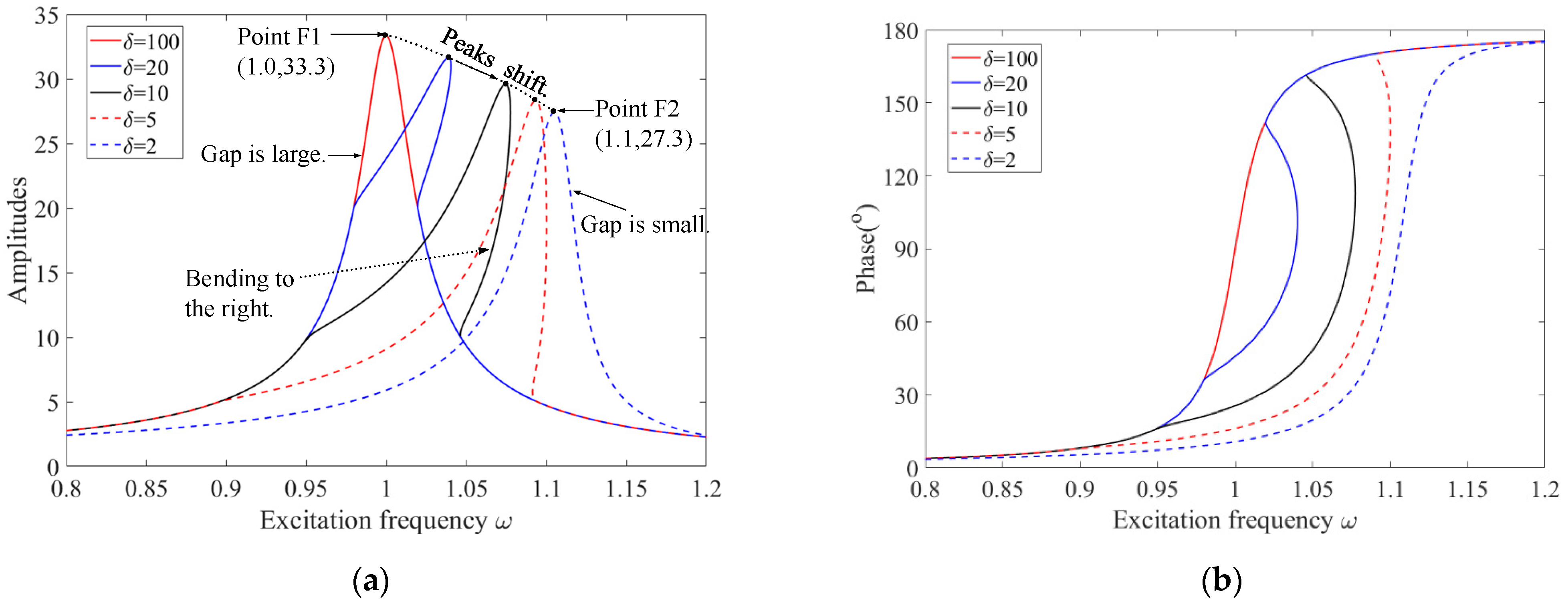
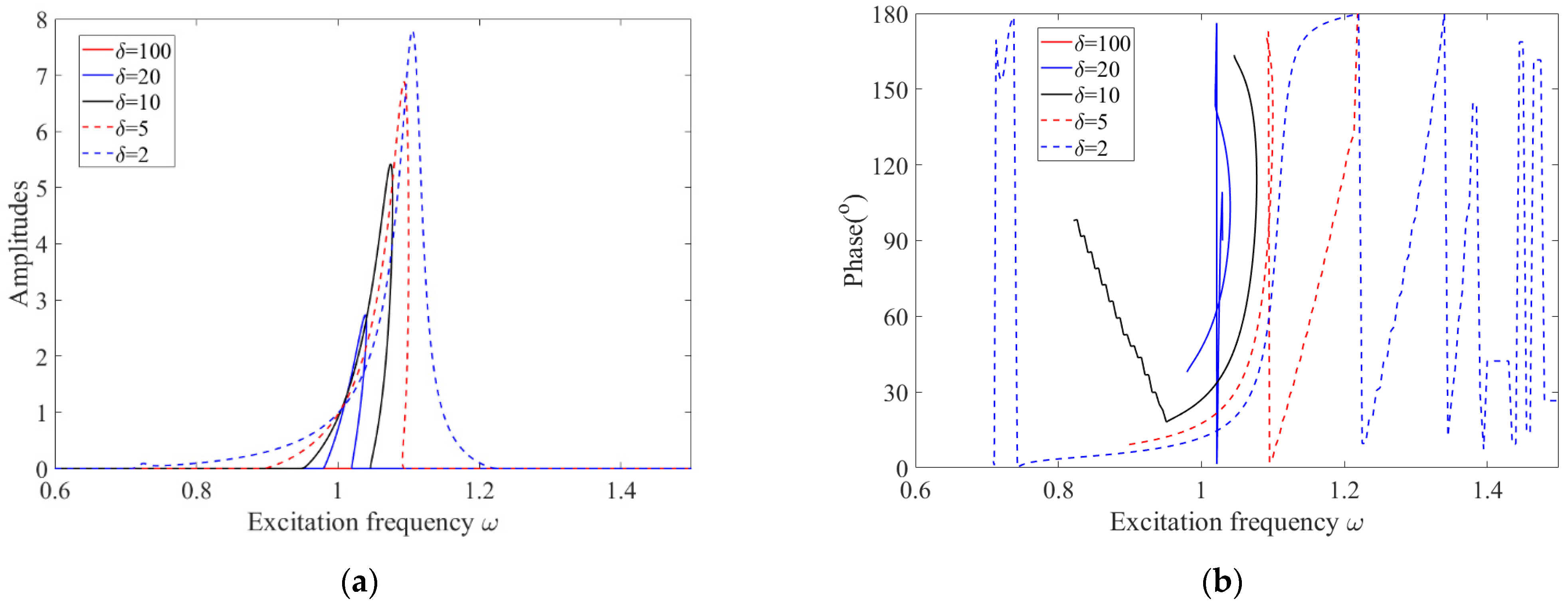
Let $\kappa$ = 1, $\delta$ = 100, 20, 10, 5, 2. The amplitude–frequency and phase–frequency characteristics are obtained using the HBM-AFT, as shown in Figure 3 and Figure 4:

(1)

When $\delta$ = 100, the gap is large enough, and Dof-1 and Dof-2 never come into contact, and the amplitude–frequency characteristic is the forced excitation response of Dof-1.

(2)

When $\delta$ < 100, Dof-1 and Dof-2 contact; the amplitudes are larger than the gap with some excitation frequencies, and the amplitude–frequency curves are similar to that of the system with a hardening spring showing the resonance peak bending to the right.

(3)

When the gap changes from 100 to 2, the peak of frequency amplitude curves shifts from point F1 to point F2, and the resonance frequency increases from 1.0 to 1.1 correspondingly.

(4)

When the gap decreases from 100 to 2, the amplitude of the resonance peaks decreases from 33.3 to 27.3 (−18%); the vibration suppression efficiency (18%) of the elastic stop structure on Dof-1 is not very good, which depends on the parameters $\kappa$, $\gamma$. In the following, the vibration suppression of an elastic stop with different stiffensses is investigated.

(5)

The phase–frequency characteristics of Dof-2 have difficulty finding a common rule.

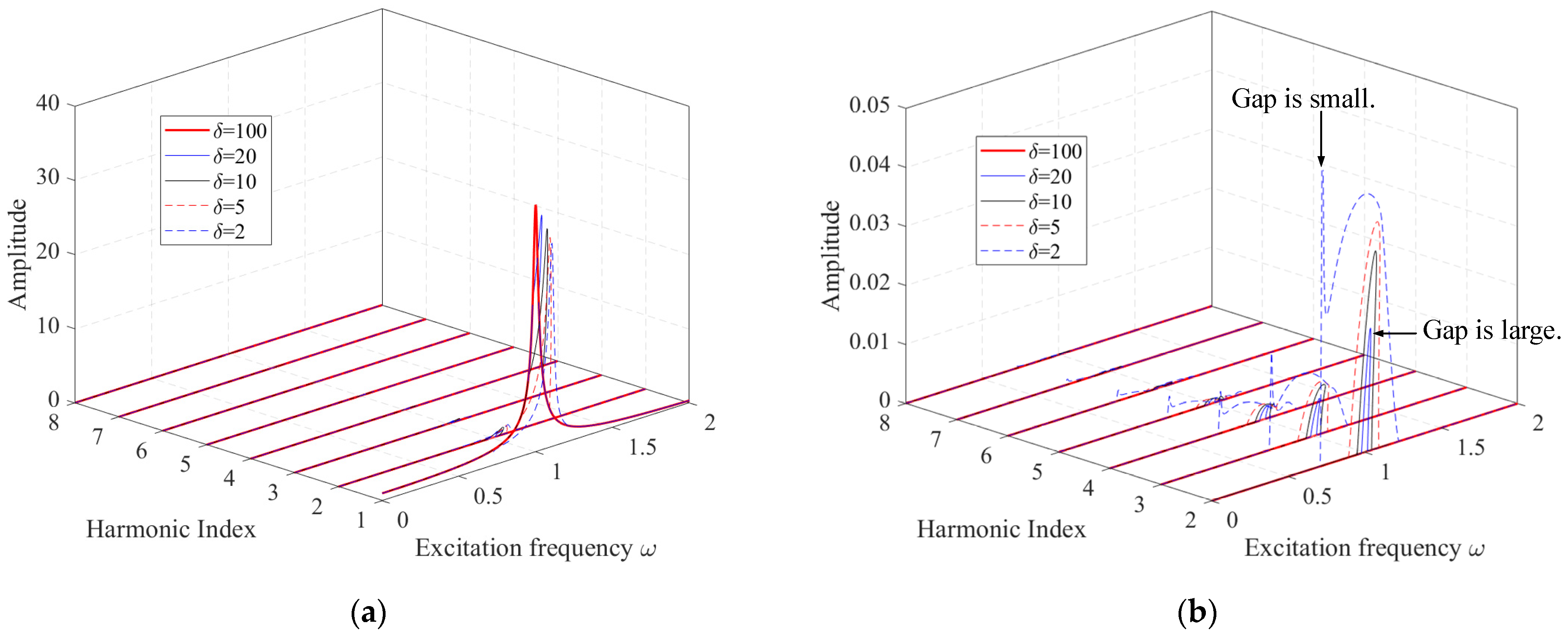
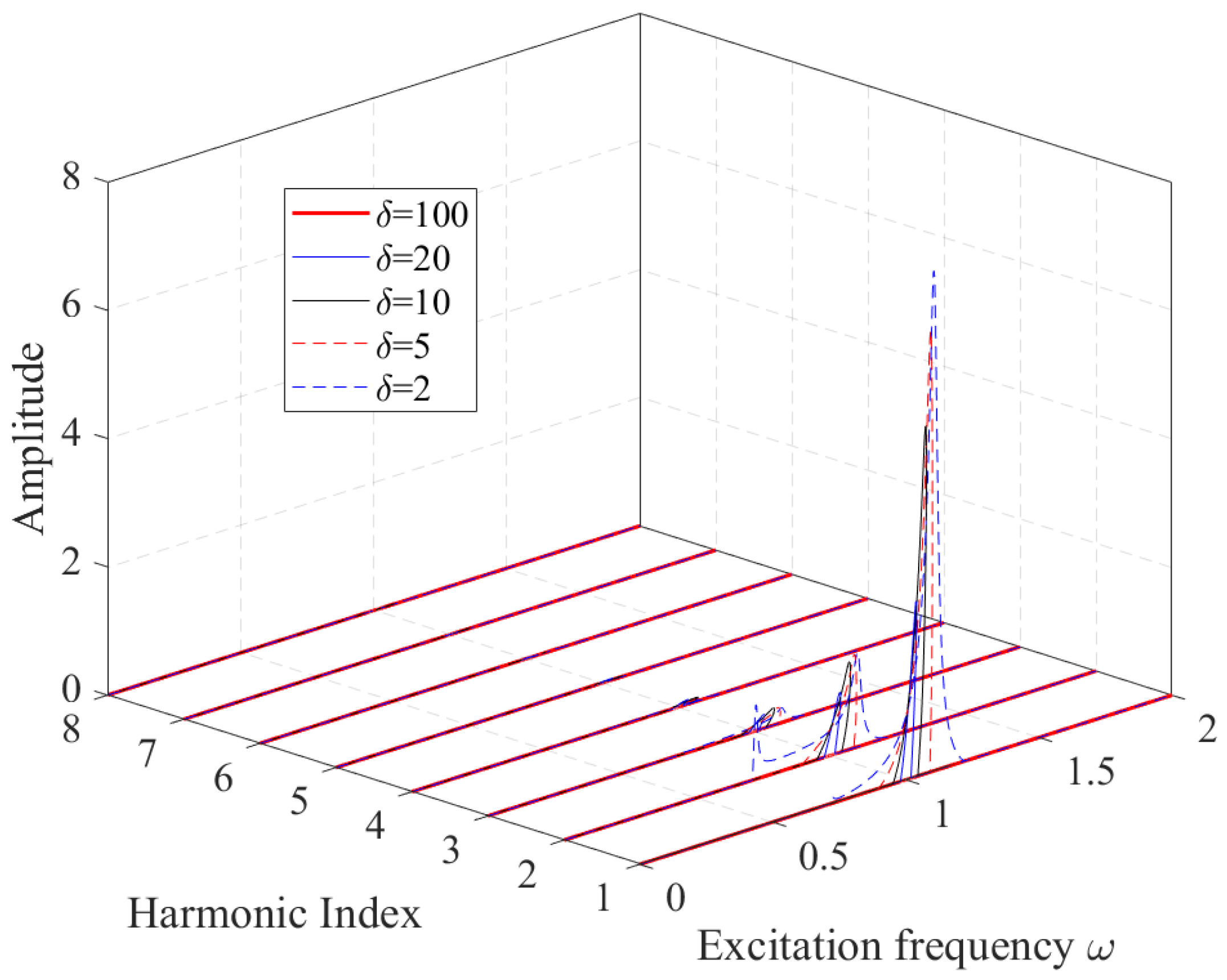
The amplitudes of the harmonic terms of each order (1~8th) are shown in Figure 5 and Figure 6, and the relative values are normalized by the amplitude of the fundamental frequency component. The harmonic index corresponds to the subscript index $k$ in Equation (8). When the harmonic index is 1, the frequency component is the fundamental frequency (denoted by 1X). When the harmonic index is higher than 1, the frequency component is the super-harmonic term. It obvious that the amplitudes of super-harmonic components are relatively smaller compared with the first order and are less than 10%. Moreover, the relative amplitudes of high-order components are larger when the gap is smaller. In the following analysis, this study focuses on the amplitudes of the first-order component.

3.2. Stability and Frequency Components

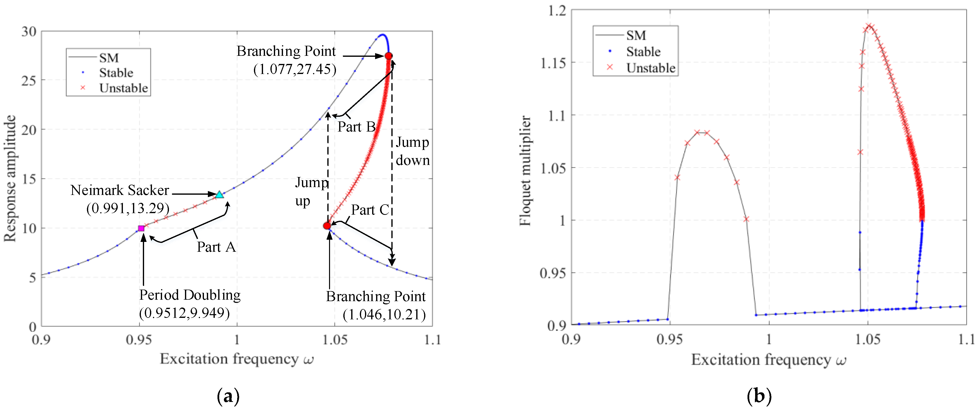
In this paper, the analysis focuses on the curves with the “bending” phenomenon. Taking $\delta$ = 10 as an example, the amplitude–frequency characteristic of the system is obtained by the shooting method (SM). The stability of the periodic solution under different excitation frequencies is analyzed according to the Floquet theory, as shown in Figure 7, with four bifurcation points, namely Period Doubling, Neimark–Sacker, Branching Point, and Branching Point. The particular parts on the amplitude–frequency curves are marked as A, B, and C to study their frequency spectra, respectively.

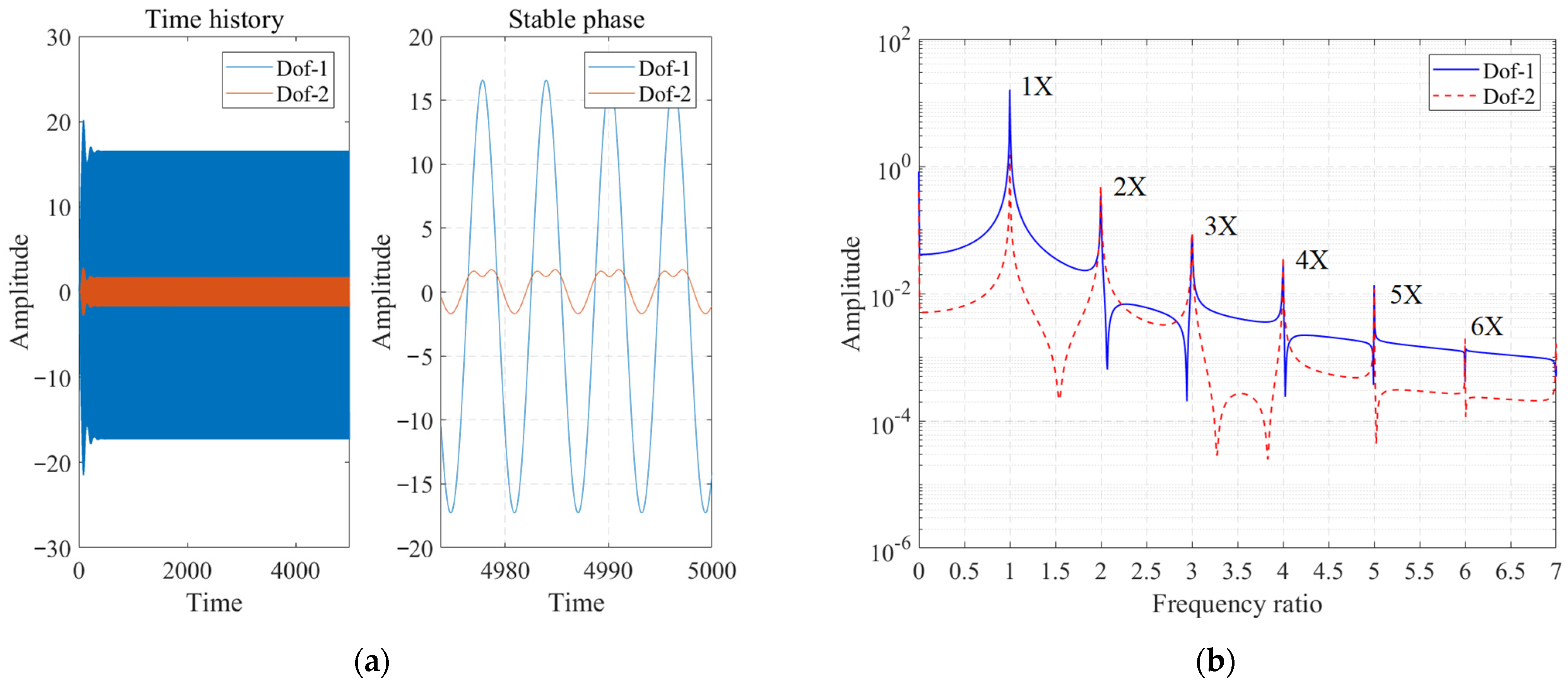
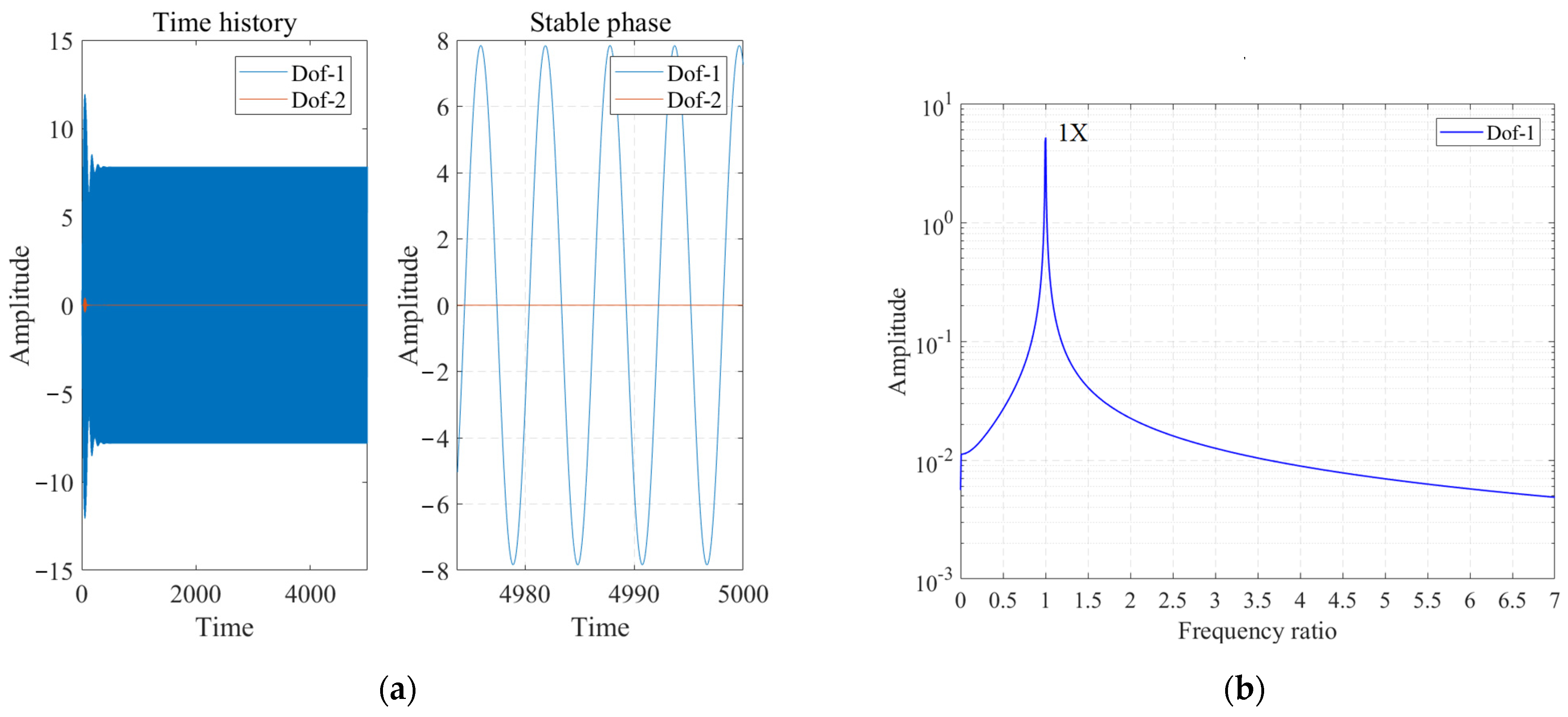
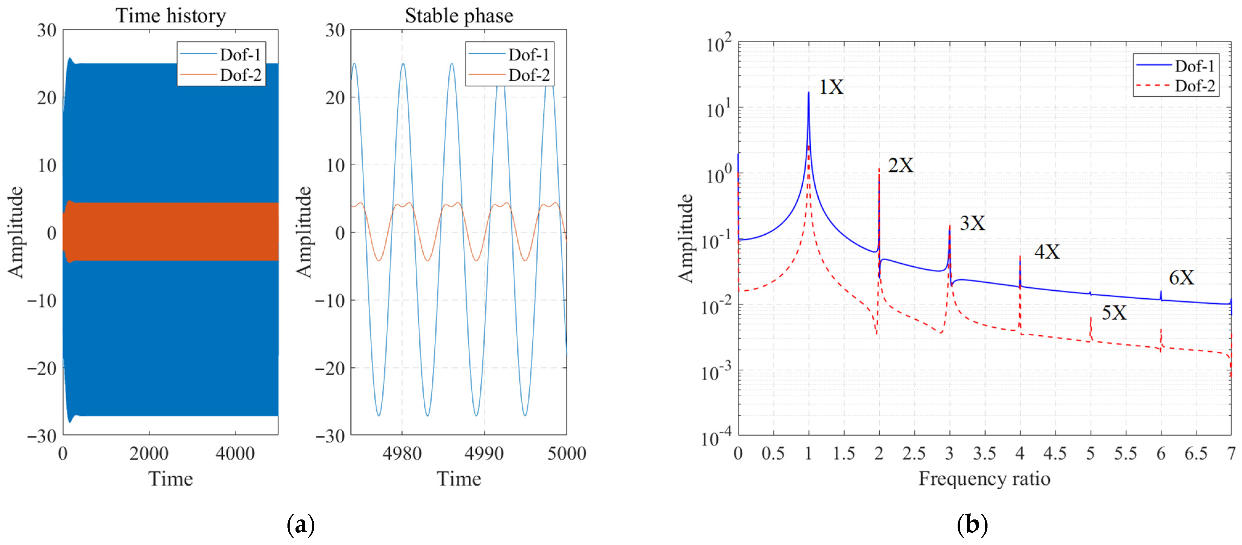
Based on the Ode15s solver in Matlab R17b, the initial displacement and velocity are 0 (if not specified). The time history and frequency spectra of the system at excitation frequencies of 0.95, 0.97, 1.02, and 1.06 are shown in Figure 8, Figure 9, Figure 10, Figure 11 and Figure 12, where the frequency spectra are normalized by the excitation frequency. When the excitation frequency is located in region A, the frequency spectrum of the system includes $0.5\omega$ and $\left(n+0.5\right)\omega$, in addition to the multiplier frequency $n\omega$; when the excitation frequency is located between 1.046 and 1.077, the curve between regions B and C cannot be realized, and the response amplitude is located in regions B or C depending on the initial value, that is to say, there can be more than one steady-state response for a given excitation frequency at these unstable points. This bi-stable regime implies the jump phenomena, and the jump point is the branching point.

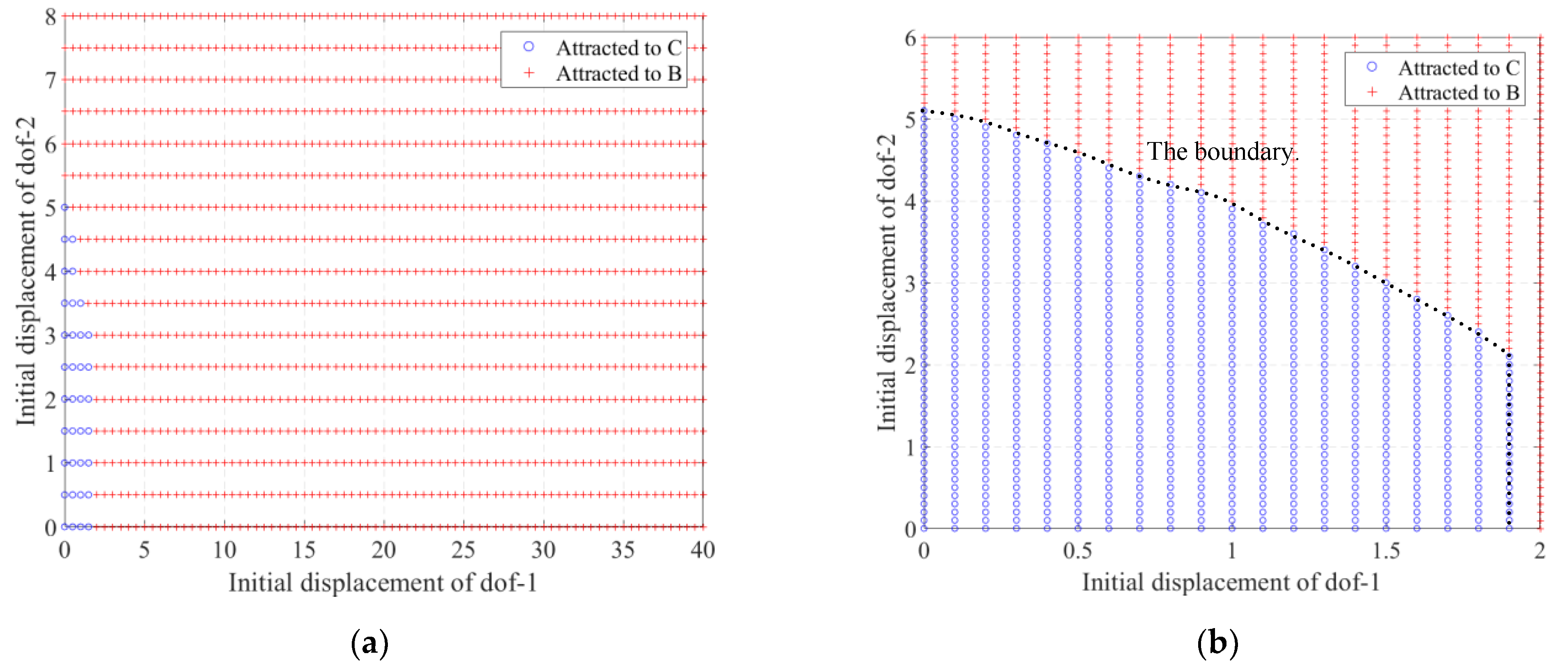
The excitation frequency of 1.06 is used as an example to explore the domain of attraction of the bi-stable periodic solution to the initial displacement, with the intervals of [0–40] and [0–8] for the initial displacements of the two Dofs. The distribution of the domain of attraction is shown in Figure 13, where the amplitude of the steady-state response tends to B is marked as red+, and C is marked as blue circles. As we can see, there exists a clear boundary between the different attractions.

3.3. Sweep Frequency Response

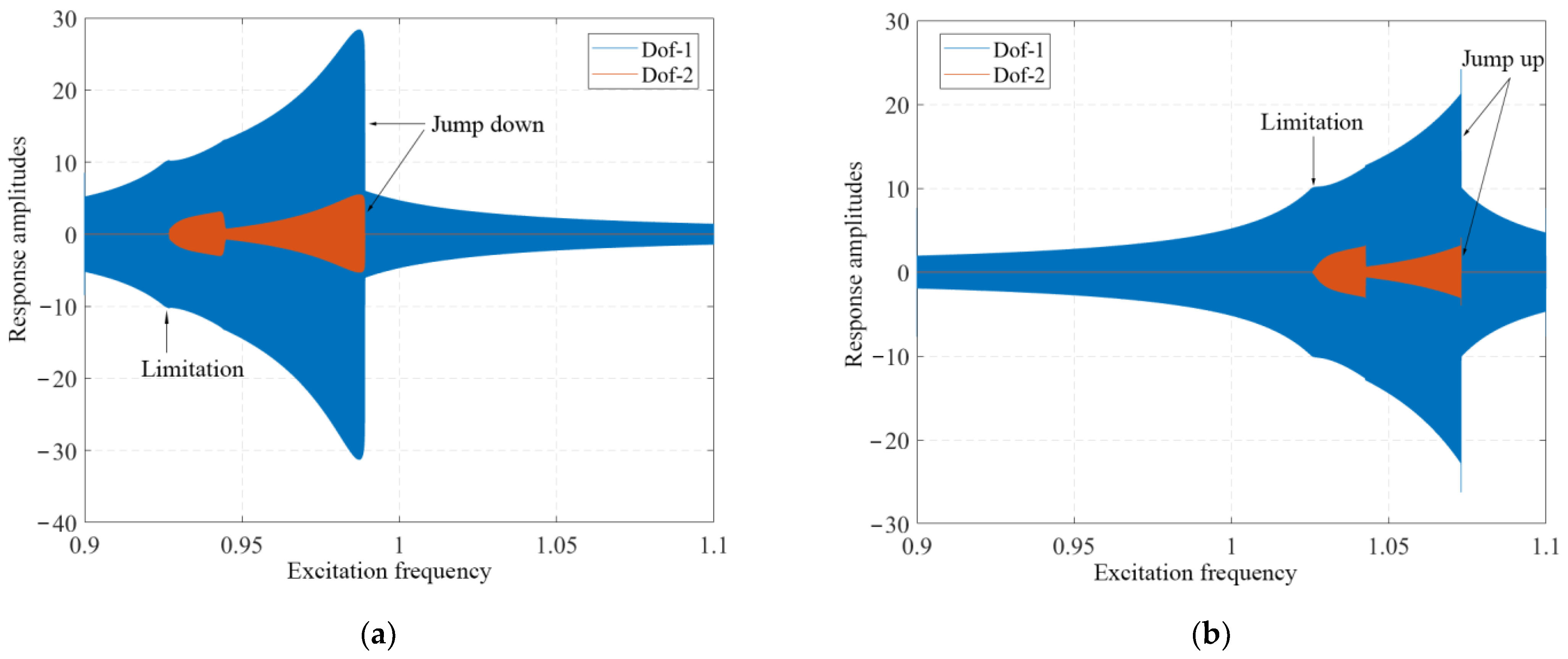
The sweep method can simulate the jump phenomenon in the process of excitation frequency increase and decrease. The Ode15s solver in Matlab is used, and the continuous sweep response of the system at the excitation frequency of 0.9–1.1, where the total time is 1$\times {10}^{6}s$, and the rate of frequency change is 2$\times {10}^{-6}{s}^{-1}$. The response of the system during the increase and decrease of the excitation frequency is shown in Figure 14, where the jump phenomenon occurs during both the increase and decrease of the excitation frequency.

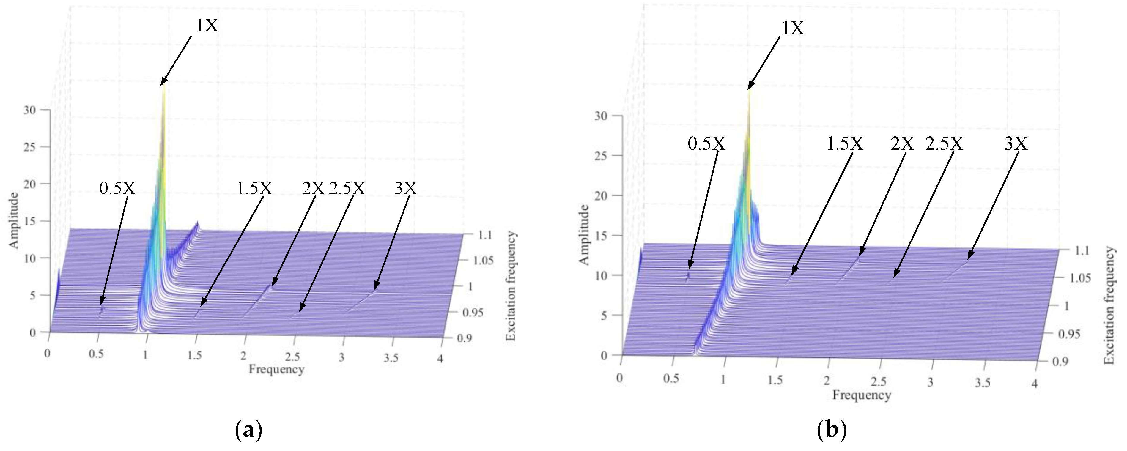
The excitation frequency–frequency spectrum–amplitude three-dimensional waterfall of Dof-1 in the continuous sweep process is shown in Figure 15, and the frequency components in the response are different in different excitation frequency intervals. The amplitude–frequency characteristics in the previous subsection correspond to the stability analysis results, that is, the excitation frequency changes from small to large: the two degrees of freedom do not contact, the frequency component is only the excitation frequency 1X; intermittent contact, the frequency component is composed of 0.5X, (n + 0.5)X and nX; intermittent contact; however, 0.5X, (n + 0.5)X disappears. In addition, it can be seen that the jump phenomenon is mainly caused by the change of the fundamental frequency amplitude. However, in the continuous sweep process, as the excitation frequency is always varying, the response is in the transient state. Therefore, the amplitude of the sweeping process is the same as the amplitude of the steady-state response at a fixed excitation frequency.

3.4. Vibration Suppression

To achieve vibration suppression, influences of the stiffness $\kappa$ and $\gamma$ on the response are studied. Taking the system with $\delta$ = 10, and $\kappa$ = 1, 2, 5, 10, 50, 1000 as an example, the amplitude–frequency and phase–frequency characteristics of Dof-1 and Dof-2 are shown in Figure 16. The stiffness $\kappa$ changes the amplitude and frequency of the resonance point to a certain extent; however, it does not change the shapes of the amplitude–frequency and phase–frequency curves. When the stiffness $\kappa$ is not smaller than 50, it can be considered as rigid as enough to design a rigid stop for the vibration suppression purpose.

The stiffness $\gamma$ of the elastic stop affects the response of the system as well. Taking $\delta$ = 10, $\kappa$= 50, and $\gamma$ = 1, 2 (original system), 10, 50, 100 as the example, the influences of stiffness on the amplitude–frequency and phase–frequency characteristics are shown in Figure 17. The stiffness $\gamma$ will not only affect the amplitude and frequency of the resonance point, but also change the shape of the amplitude–frequency and phase–frequency curves. However, the amplitude–frequency curve is roughly similar to the system with a hardening spring. When the stiffness $\gamma$ is not less than 10, the response amplitudes of Dof-1 are not large than 13.7, which is very close to the limit amplitude of 10. Therefore, to realize the amplitude suppression of primary system of the Dof-1 based on the impact damper of Dof-2, it is necessary to reasonably design the stiffness $\kappa$ and $\gamma$ of the elastic stop, and comprehensively consider the amplitude of the full frequency range and the position of the resonance point.

4. Application to a Flexible Rotor

In this section, the nonlinear dynamics of the impact system are applied to a flexible rotor–support system considering the pedestal–looseness fault. The rotor is modeled based on the finite element method using Timoshenko’s thick beam formulation, and the pedestal–looseness fault is considered by the nonlinearity of an elastic stop. In the meantime, the loosed pedestal designed artificially can be used for the purpose of vibration suppression.

4.1. Model of the Rotor

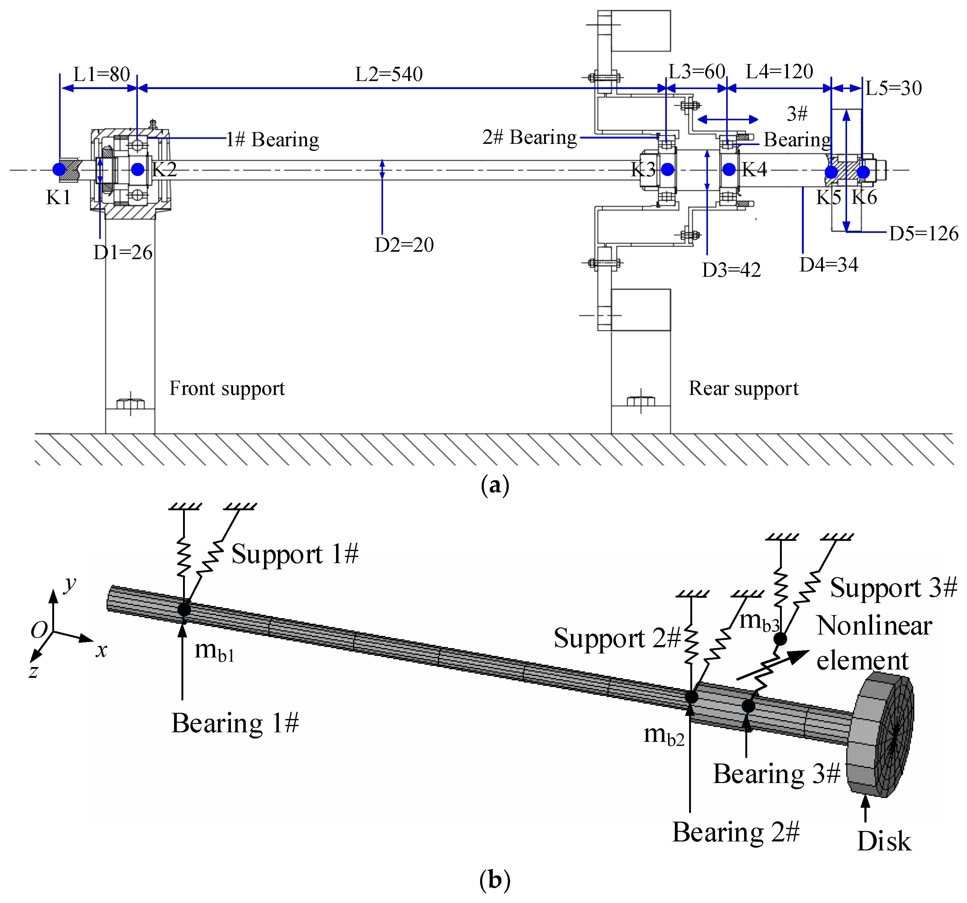
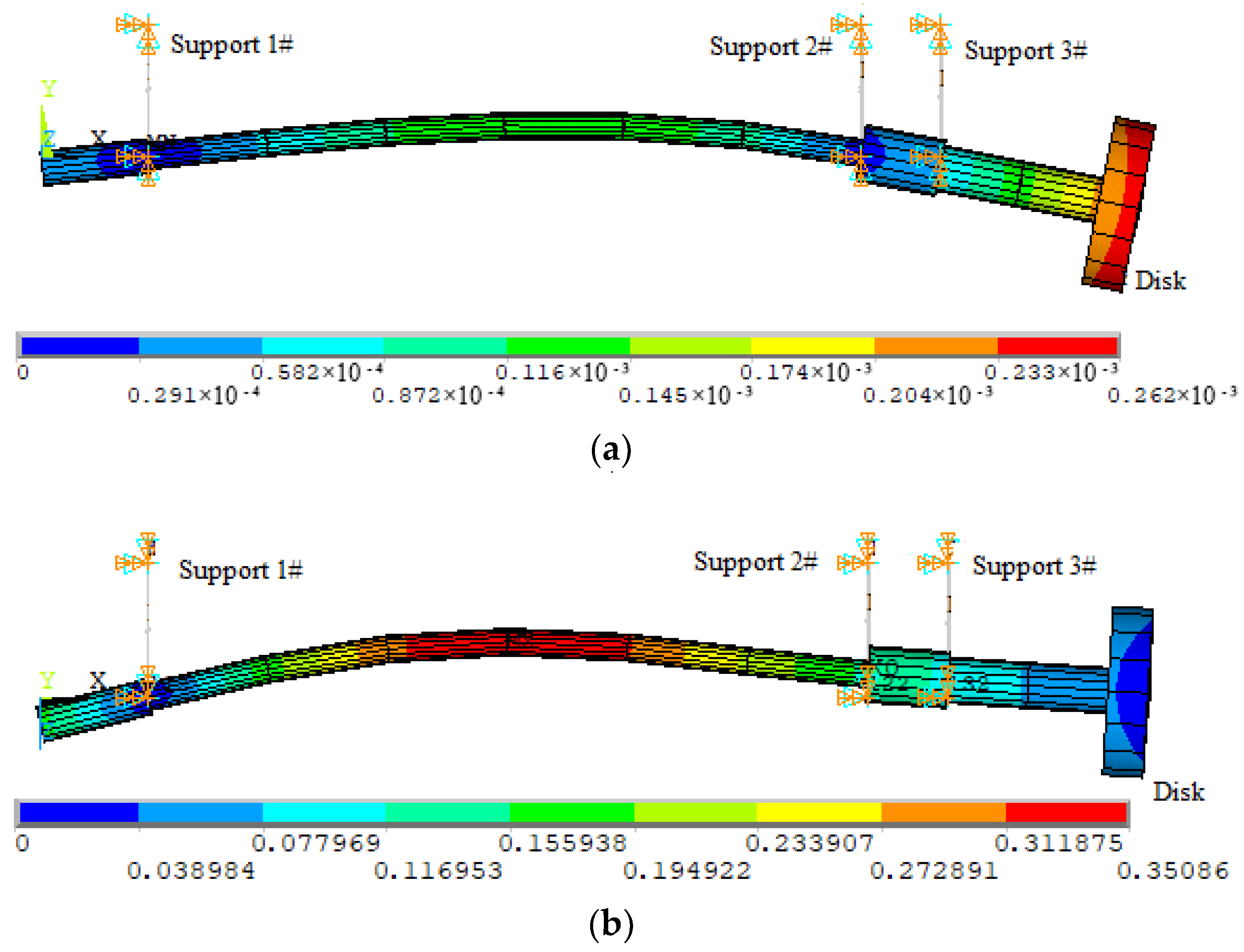
A flexible rotor–support system is shown in Figure 18. There exist three bearings: 1# bearing, 2# bearing, and 3# bearing. The 1# bearing is ball bearing, 2# and 3# bearing are roller bearing. The material is assumed to be 45# steel, of which the density is 7800 kg/mm³ and the elastic modulus is 210 Gpa. The stiffness of the 1# bearing-support is 1 × 10⁸ N/m, and the stiffness of the 2# and 3# bearing-support is 3 × 10⁶ N/m. The mass of the 1# pedestal is 2 kg (m_b1) and the masses of the 2# and 3# pedestal are 1 kg (m_b2) and 1.5 kg (m_b3), respectively. In Ansys19.0, the beam element Beam188 is used to model the rotor shaft, the Combin14 element is used to simulate the support, and the Mass21 element is used to simulate the pedestal mass. The first and second order natural vibration modes of the derived linear rotor system are shown in Figure 19, and the corresponding natural frequencies are 57.6 Hz and 159.7 Hz. In engineering, the rotor is often operating above the first critical speed; thus, the excitation frequencies near the first resonance peak are focused on in the following analysis.

To analyze the nonlinear behavior, the model of elastic stop is introduced into the governing equations at the node of 3# bearing. The governing equations can be derived by using the method in Appendix B and are as follows:

$$M\ddot{q}+\left(C+\omega G\right)\dot{q}+Kq+F_{nl}=F_{ex}$$

(21)

in which M, ωG, and K are the matrix of mass, gyroscopic moment, and stiffness, and are obtained by the finite element method; C is the damping matrix and is obtained by

$$C=c_{\alpha }M+c_{\beta }K$$

(22)

$$c_{\alpha }=\frac{2\zeta {\omega }_1{\omega }_2}{{\omega }_1+{\omega }_2}$$

(23)

$$c_{\beta }=\frac{2\zeta }{{\omega }_1+{\omega }_2}$$

(24)

$\zeta$ is damping ratio, which is 0.03 in this paper; ${\omega }_1$ and ${\omega }_2$ are the lower and upper bounds of the considered frequency, which are 62.8 rad/s(10 Hz) and 6283.2 rad/s(1000 Hz) in this paper.

$F_{\mathrm{ex}}$ is the unbalance excitation force; $F_{nl}$ is the nonlinear force caused by elastic stop model and is expressed as

$$F_{\mathrm{nl}}=k_p\left(1-\frac{\delta }{r}\right)f_c\left(r-\delta \right)\left(w_1\left(w_1^{T}q\right)+w_2\left(w_2^{T}q\right)\right)$$

(25)

$w_1$ and $w_2$ are the vectors indicating the direction of the nonlinear force in the system; $r$ is the radial displacement amplitude and is calculated by

$$r=\sqrt{{\left(w_1\left[x\right]\right)}^2+{\left(w_2\left[x\right]\right)}^2}$$

(26)

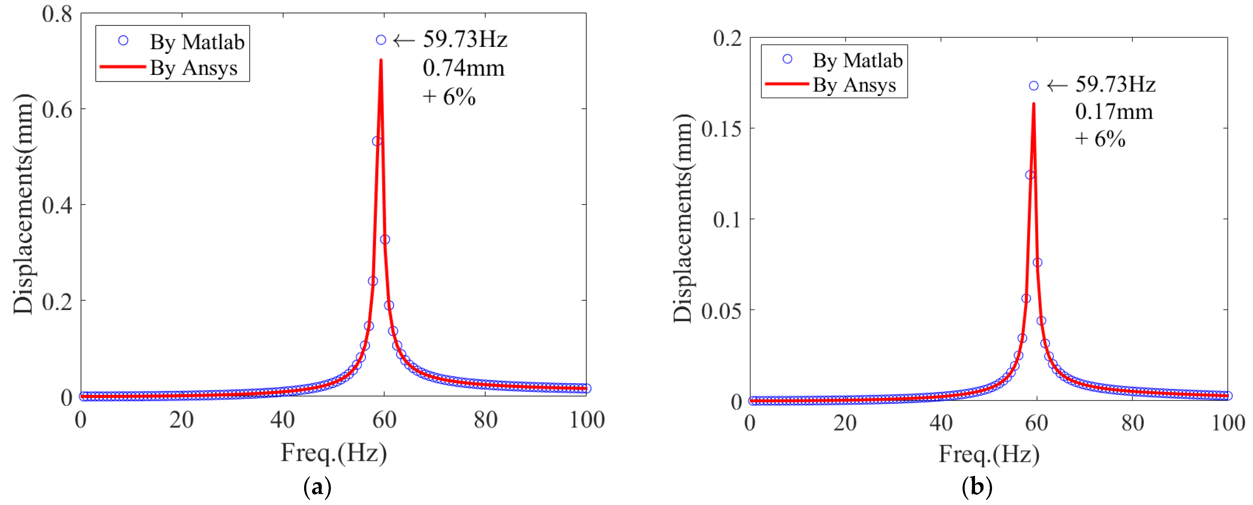
The harmonic responses of the linear system without pedestal looseness are obtained by Ansys19.0 and MatlabR2017b (the program of the HBM method in Section 2.2), respectively. In the analysis, the unbalance forces are located at the disk and the middle of the shaft, and the unbalanced forces are 10 g·mm. The response of the disk and the support of 3# bearing are shown in Figure 20. The frequency of the resonance peak is 59.7 Hz due to the gyroscopic effect. The amplitudes obtained by Matlab are higher than the one obtained by Ansys by the ratio of 6%, which verifies the solving method.

4.2. Amplitude–Frequency Characteristics

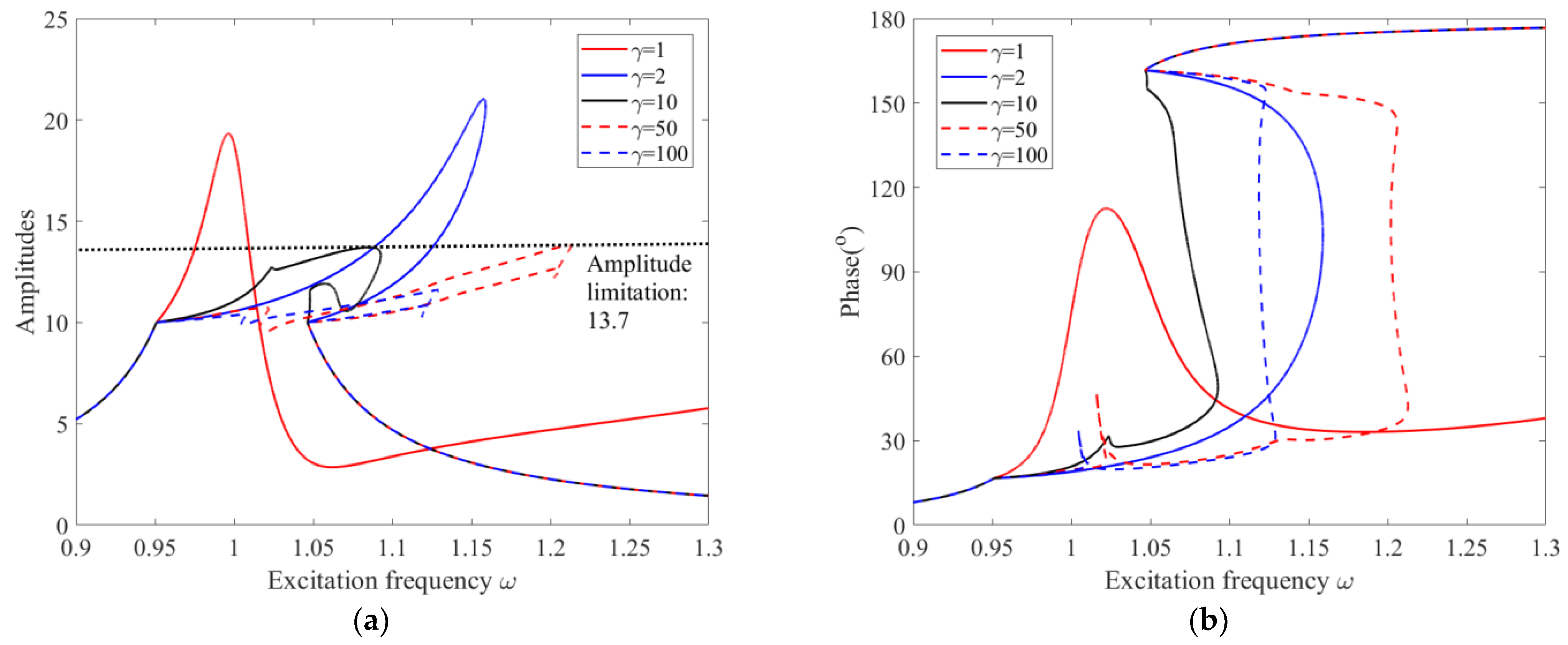
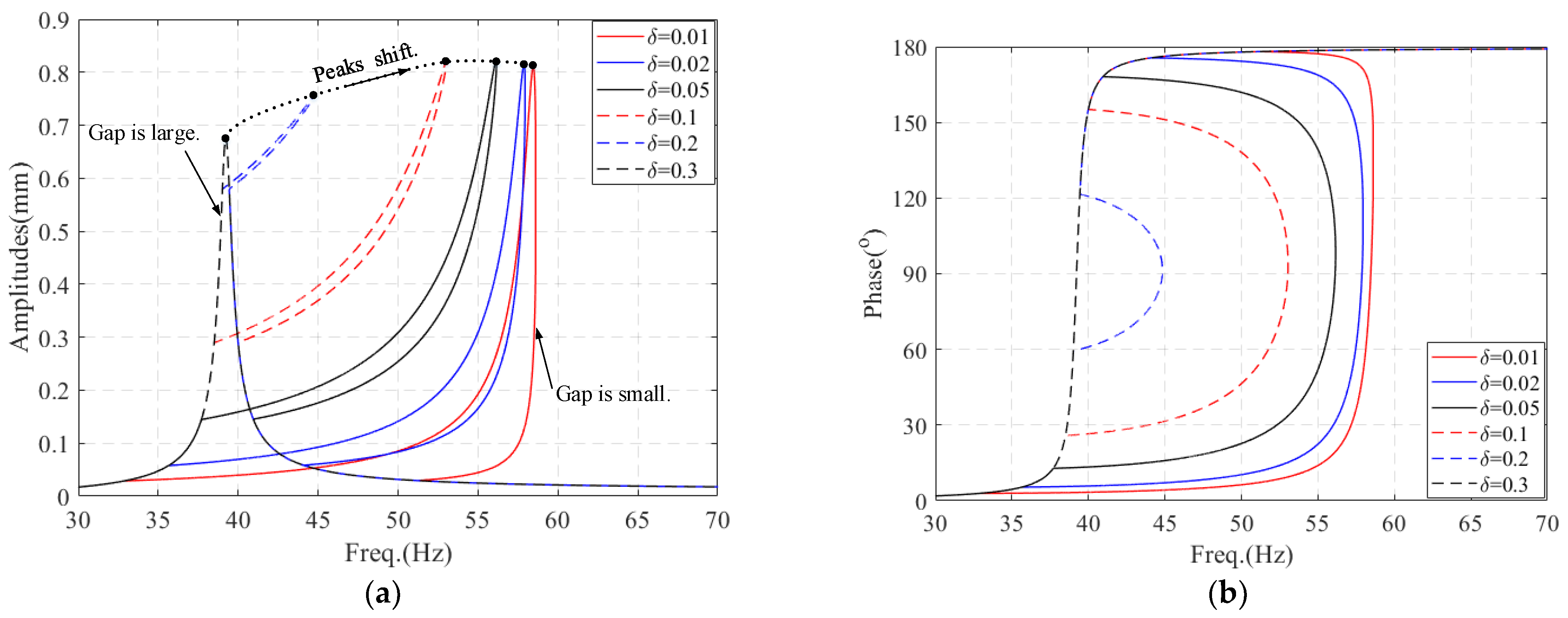
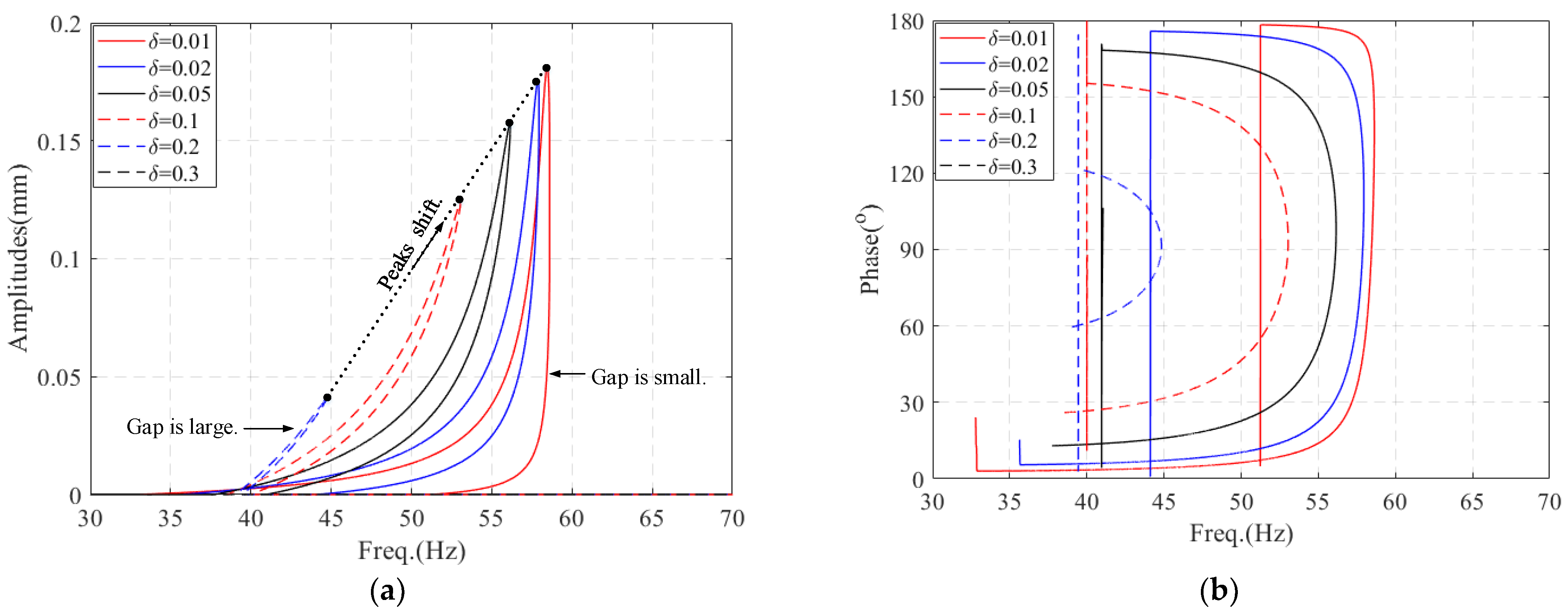
Let k_p = 3 × 10⁸ N/m (100 times of stiffness of 3# bearing-support), and δ = 0.01, 0.02, 0.03, 0.05, 0.1, 0.2, 0.3 mm. The amplitude–frequency and phase–frequency characteristics of the disk and the 3# bearing-support are obtained using the HBM-AFT, as shown in Figure 21 and Figure 22: As the gap size decreases, the resonance point gradually shifts to the right, while the amplitude of the resonance point does not change too much. This phenomenon is similar to the result of the mechanism model in Section 3.

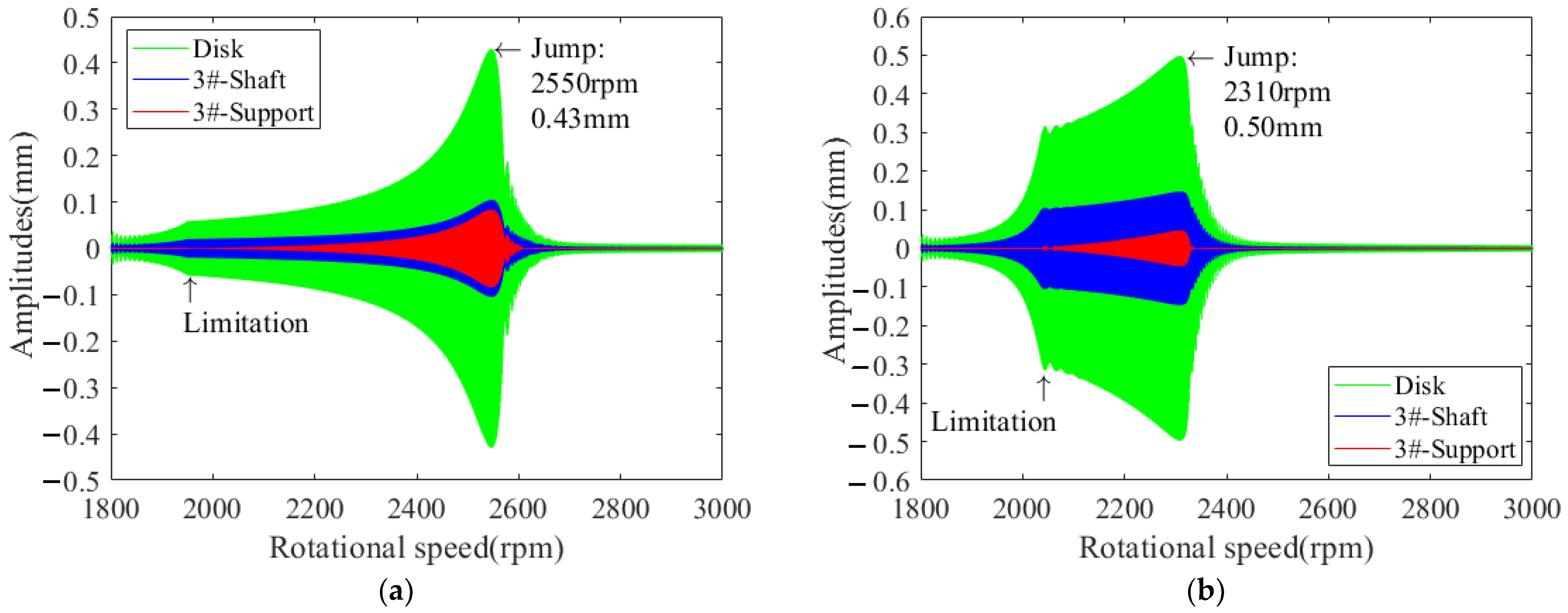
The frequency sweep method is used to simulate the jump phenomenon in the process of speeding up, and Ode15s in Matlab R17b is chosen as the solver. The transient response of the system is obtained with the rotational speed range of 1800–4200 rpm (30–70 Hz). The total time span is 20 s, and the speed change rate is 60 rpm/s. The time history responses of the system with a small clearance of 0.02 mm and a large clearance of 0.1 mm are as shown in Figure 23a,b. The results are consistent with the results of amplitude–frequency curves obtained by HBM, by comparing the small gap of 0.02 mm and the large gap of 0.1 mm.

4.3. Vibration Suppression

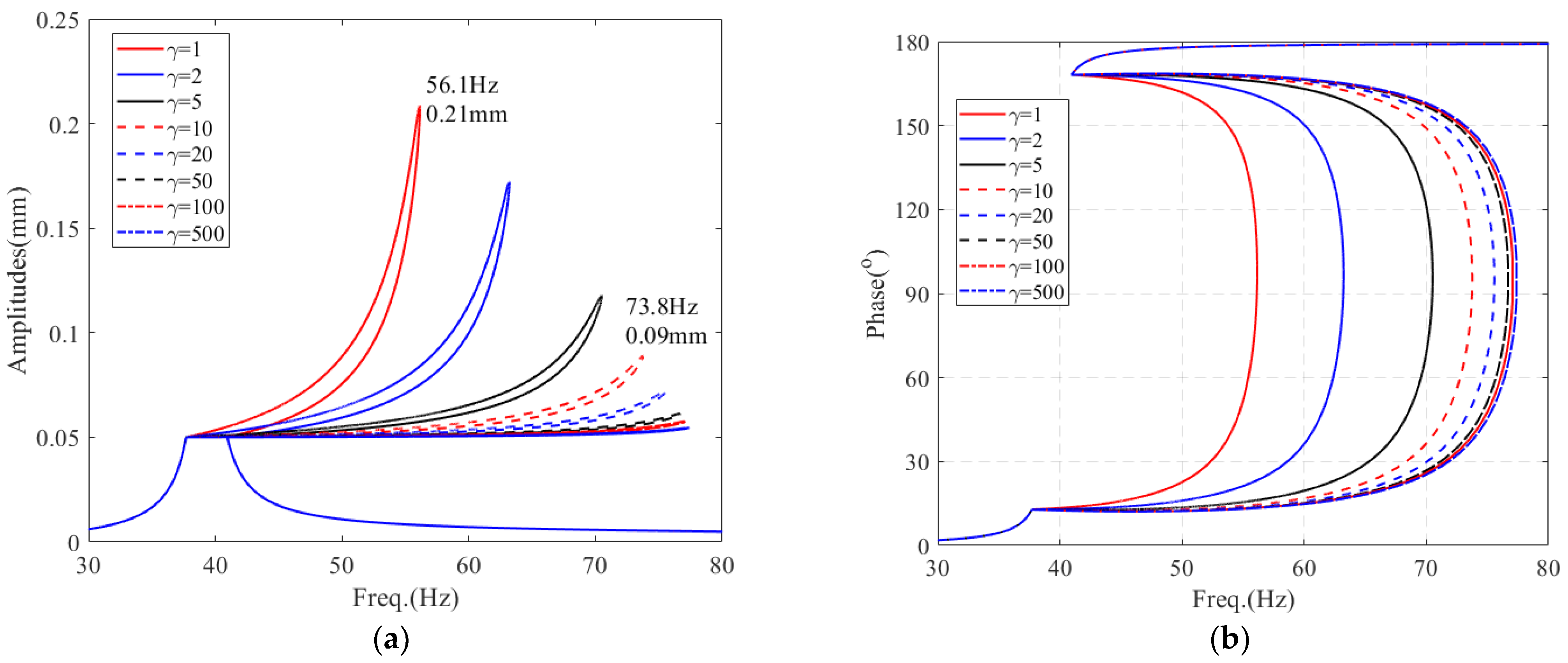
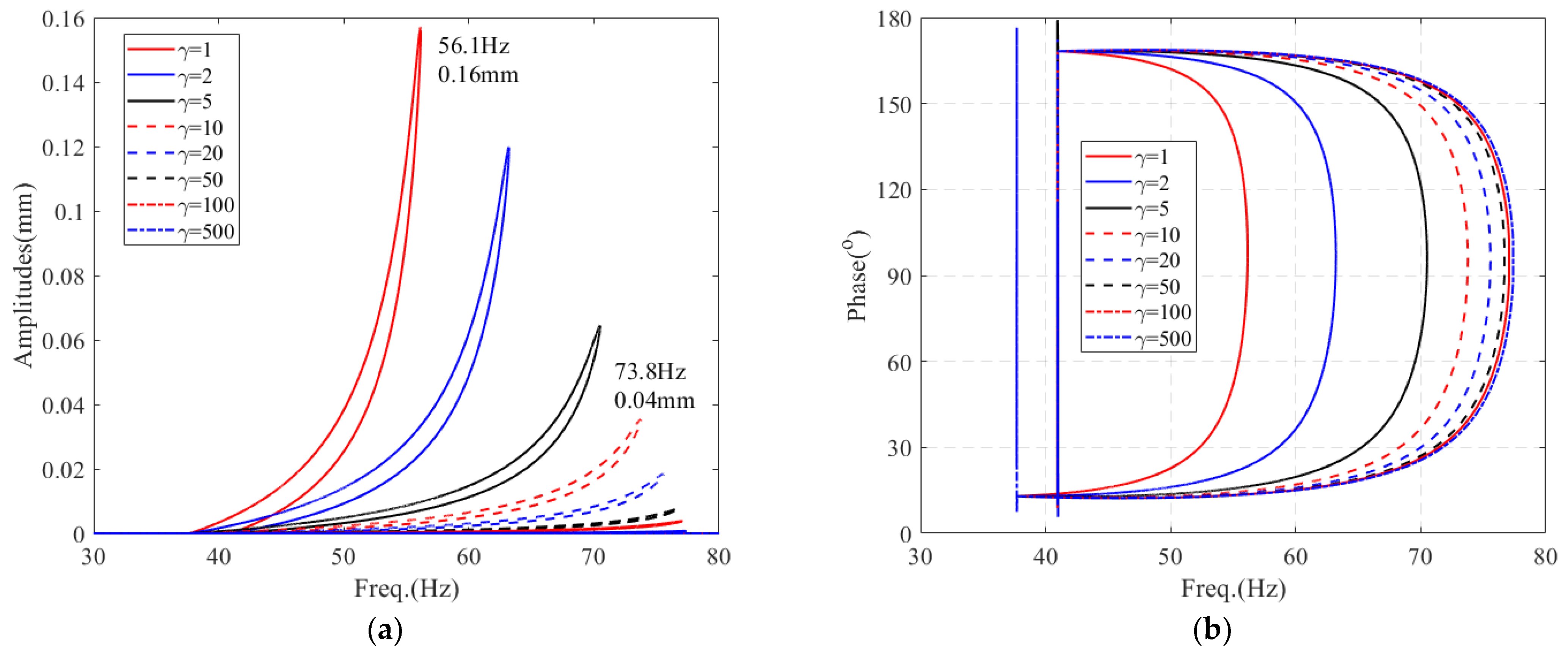
According to the research results of the mechanism model in Section 3, it can be seen that the effect of the elastic support is closely related to the stiffness of the 3# support. Thus, a stiffness coefficient γ is set, indicating that the stiffness of 3# support is γ times of the original stiffness (3 × 10⁶ N/m). Taking γ = 1 (the original system), 2, 5, 10, 20, 50, 100, 500 as the example, the influences of 3# support stiffness on the amplitude–frequency and phase–frequency characteristics are shown in Figure 24 and Figure 25. As the stiffness of 3# support increases, the resonance point amplitude at the 3# support gradually decreases, and the resonance point shifts to the right gradually. When the 3# support stiffness is the original one with 3 × 10⁶ N/m, the frequency of the resonance point is 56.1 Hz and the amplitude is 0.21 mm; when the 3# support stiffness is 10 times (3 × 10⁷ N/m) that of the original one, the frequency of the resonance point is 73.8 Hz, and the amplitude is 0.09 mm, which is 57% lower than the amplitude of the original system. In addition, the amplitude is close to the limit of 0.05 mm, when the 3# support stiffness is not less than 3 × 10⁷ N/m.

The vibration suppression of 3# support is of great significance for reducing the dynamic load of the local structure near 3# support and controlling the local deformation of the support structure. However, when the vibration suppression of the rotor–support system is realized through the design of the elastic stop, it is necessary to reasonably design every single parameter, and comprehensively consider the deformation of each key position of the rotor–support system.

5. Conclusions

In this paper, a novel vibro-impact system with an elastic stop present by piecewise-type nonlinearities is promoted, and its vibration behaviors are studied in detail. From the results, some useful conclusions can be drawn, which can give some guidance on predicting resonance frequencies and amplitudes, analyzing frequency components, detecting faults, and suppressing vibration.

(1)

As for the frequency amplitude response, the amplitude–frequency curve of a system with an elastic stop is similar to the system with a hardening spring showing the resonance peak bending to the right. As for the “bending” curves, the periodic solution is unstable, and there can be more than one steady-state response for a given excitation frequency, and jumps occur in the process of speed-up and speed-down. In engineering, it is important to be concerned about the jumping phenomenon in a system with gaps.

(2)

When the gap becomes small gradually, the resonance peak shifts from a low frequency to a high frequency, and the amplitude of the resonance peaks decreases. Thus, it is feasible to use an elastic stop for suppressing vibration in practical applications. However, the stiffness of the elastic stop will influence the efficiency of suppression, and the characteristics of the elastic stop should be designed properly.

(3)

In addition, at the unstable point, the frequency spectrum includes 0.5X, (n + 0.5)X and nX, in addition to the fundamental frequency 1X; and investigating frequency components is an effective method for detecting vibration faults induced by gaps.

(4)

The amplitudes of super-harmonic components are relatively smaller compared with the fundamental frequency, and are less than 10%. Moreover, the relative amplitudes of high-order components are larger when the gap is smaller. Thus, in most cases of engineering problems, it will be useful to focus on the fundamental frequency component if excess vibration occurs and vibration suppression is required.

(5)

The application of the elastic stop to a specific rotor support system is investigated. A new pedestal loosening rotor with an overhanging disk and three supports is promoted and investigated. The dynamic responses of the rotor with an elastic stop are similar to that of the two-Dof model with piecewise linear functions. In the meantime, the feasibility of vibration suppression of a flexible rotor by using an elastic stop has been verified in this paper.

Therefore, the results of this paper can not only explain some dynamic behaviors of the system with an elastic stop, but also provide some guidance for the design of impact dampers in engineering.

References

- Thompson, J.; Ghaffari, R. Chaos after period-doubling bifurcations in the resonance of an impact oscillator. Phys. Lett. A 1982, 91, 5–8. [Google Scholar] [CrossRef]
- Thompson, J.M.T. Complex dynamics of compliant off-shore structure. Proc. Proc. R. Soc. Lond. Math. Phys. Sci. F 1983, 50, 849–857. [Google Scholar]
- Shaw, S.; Holmes, P. A periodically forced impact oscillator with large dissipation. J. Appl. Mech. 1983, 50, 849–857. [Google Scholar] [CrossRef]
- Shaw, S.W.; Holmes, P. A periodically forced piecewise linear oscillator. J. Sound Vib. 1983, 90, 129–155. [Google Scholar] [CrossRef] [Green Version]
- Hindmarsh, M.; Jefferies, D. On the motions of the offset impact oscillator. J. Phys. A Math. Gen. 1984, 17, 1791–1804. [Google Scholar] [CrossRef]
- Peterka, F. Dynamics of oscillator with soft impacts. Int. Des. Eng. Tech. Conf. Comput. Inf. Eng. Conf. 2001, 80296, 2639–2645. [Google Scholar]
- Bapat, C. Exact solution of stable periodic one contact per N cycles motion of a damped linear oscillator contacting a unilateral elastic stop. J. Sound Vib. 2008, 314, 803–820. [Google Scholar] [CrossRef]
- Kong, X.; Sun, W.; Wang, B.; Wen, B. Dynamic and stability analysis of the linear guide with time-varying, piecewise-nonlinear stiffness by multi-term incremental harmonic balance method. J. Sound Vib. 2015, 346, 265–283. [Google Scholar] [CrossRef]
- Wang, S.; Hua, L.; Yang, C.; Han, X.; Su, Z. Applications of incremental harmonic balance method combined with equivalent piecewise linearization on vibrations of nonlinear stiffness systems. J. Sound Vib. 2019, 441, 111–125. [Google Scholar] [CrossRef]
- Aidanpää, J.-O.; Gupta, R. Periodic and chaotic behaviour of a threshold-limited two-degree-of-freedom system. J. Sound Vib. 1993, 165, 305–327. [Google Scholar] [CrossRef]
- Natsiavas, S. Dynamics of multiple-degree-of-freedom oscillators with colliding components. J. Sound Vib. 1993, 165, 439–453. [Google Scholar] [CrossRef] [Green Version]
- Luo, G.-W.; Xie, J.-H. Hopf bifurcation of a two-degree-of-freedom vibro-impact system. J. Sound Vib. 1998, 213, 391–408. [Google Scholar] [CrossRef] [Green Version]
- Valente, A.X.C.; Mcclamroch, N.; Mezić, I. Hybrid dynamics of two coupled oscillators that can impact a fixed stop. Int. J. Non-Linear Mech. 2003, 38, 677–689. [Google Scholar]
- Pascal, M. Analytical Investigation of the Dynamics of a Nonlinear Structure with Two Degree of Freedom. In Proceedings of the International Design Engineering Technical Conferences and Computers and Information in Engineering Conference, F, Long Beach, CA, USA, 24–28 September 2005; pp. 1959–1967. [Google Scholar]
- Pascal, M. Dynamics and stability of a two degree of freedom oscillator with an elastic stop. J. Comput. Nonlinear Dyn. 2006, 1, 94–102. [Google Scholar] [CrossRef] [Green Version]
- Brake, M.R. A hybrid approach for the modal analysis of continuous systems with discrete piecewise-linear constraints. J. Sound Vib. 2011, 330, 3196–3221. [Google Scholar] [CrossRef]
- Li, X.; Liu, K.; Xiong, L.; Tang, L. Development and validation of a piecewise linear nonlinear energy sink for vibration suppression and energy harvesting. J. Sound Vib. 2021, 503, 116104. [Google Scholar] [CrossRef]
- Ing, J.; Pavlovskaia, E.; Wiercigroch, M.; Banerjee, S. Bifurcation analysis of an impact oscillator with a one-sided elastic constraint near grazing. Phys. D Nonlinear Phenom. 2010, 239, 312–321. [Google Scholar] [CrossRef]
- Bureau, E.; Schilder, F.; Elmegård, M.; Santos, I.F.; Thomsen, J.J.; Starke, J. Experimental bifurcation analysis of an impact oscillator—Determining stability. J. Sound Vib. 2014, 333, 5464–5474. [Google Scholar] [CrossRef]
- Tan, J.; Michael Ho, S.C.; Zhang, P.; Jiang, J. Experimental study on vibration control of suspended piping system by single-sided pounding tuned mass damper. Appl. Sci. 2019, 9, 285. [Google Scholar] [CrossRef] [Green Version]
- Yoon, J.Y.; Kim, B. Vibro-impact energy analysis of a geared system with piecewise-type nonlinearities using various parameter values. Energies 2015, 8, 8924–8944. [Google Scholar] [CrossRef] [Green Version]
- Pei, L.; Chong, A.S.; Pavlovskaia, E.; Wiercigroch, M. Computation of periodic orbits for piecewise linear oscillator by Harmonic Balance Methods. Commun. Nonlinear Sci. Numer. Simul. 2022, 108, 106220. [Google Scholar] [CrossRef]
- Amer, T.S.; Starosta, R.; Almahalawy, A.; Elameer, A.S. The stability analysis of a vibrating auto-parametric dynamical system near resonance. Appl. Sci. 2022, 12, 1737. [Google Scholar] [CrossRef]
- Abdelhfeez, S.A.; Amer, T.S.; Elbaz, R.F.; Bek, M.A. Studying the influence of external torques on the dynamical motion and the stability of a 3DOF dynamic system. Alex. Eng. J. 2022, 61, 6695–6724. [Google Scholar] [CrossRef]
- Goldman, P.; Muszynska, A. Analytical and experimental simulation of loose pedestal dynamic effects on a rotating machine vibrational response. In Proceedings of the International Design Engineering Technical Conferences and Computers and Information in Engineering Conference, F; American Society of Mechanical Engineers: New York, NY, USA, 1991; pp. 11–17. [Google Scholar]
- Muszynska, A.; Goldman, P. Chaotic responses of unbalanced rotor/bearing/stator systems with looseness or rubs. Chaos Solitons Fractals 1995, 5, 1683–1704. [Google Scholar] [CrossRef]
- Chu, F.; Tang, Y. Stability and non-linear responses of a rotor-bearing system with pedestal looseness. J. Sound Vib. 2001, 241, 879–893. [Google Scholar] [CrossRef]
- Lu, W.X.; Chu, F.L. Experimental investigation of pedestal looseness in a rotor-bearing system. In Proceedings of the Key Engineering Materials, F; Trans Tech Publications: Zürich, Switzerland, 2009; pp. 599–605. [Google Scholar]
- Ma, H.; Zhao, X.; Teng, Y.; Wen, B. Analysis of dynamic characteristics for a rotor system with pedestal looseness. Shock Vib. 2011, 18, 13–27. [Google Scholar] [CrossRef]
- Lu, K.; Jin, Y.; Chen, Y.; Cao, Q.; Zhang, Z. Stability analysis of reduced rotor pedestal looseness fault model. Nonlinear Dyn. 2015, 82, 1611–1622. [Google Scholar] [CrossRef]
- Wang, H.; Chen, G. Certain type turbofan engine whole vibration model with support looseness fault and casing response characteristics. Shock Vib. 2014, 2014, 683469. [Google Scholar] [CrossRef] [Green Version]
- Chen, G. Vibration modelling and verifications for whole aero-engine. J. Sound Vib. 2015, 349, 163–176. [Google Scholar] [CrossRef]
- Chen, G.; Qu, M. Modeling and analysis of fit clearance between rolling bearing outer ring and housing. J. Sound Vib. 2019, 438, 419–440. [Google Scholar] [CrossRef]
- Wang, H.; Guan, X.; Chen, G.; Gong, J.; Yu, L.; Yuan, S.; Zhu, Z. Characteristics analysis of rotor-rolling bearing coupled system with fit looseness fault and its verification. J. Mech. Sci. Technol. 2019, 33, 29–40. [Google Scholar] [CrossRef]
- Cameron, T.M.; Jerry, H.G. An alternating frequency/time domain method for calculating the steady-state response of nonlinear dynamic systems. J. Appl. Mech. 1989, 56, 149–154. [Google Scholar] [CrossRef] [Green Version]
- Kim, Y.; Noah, S. Stability and bifurcation analysis of oscillators with piecewise-linear characteristics: A general approach. J. Appl. Mech. 1991, 58, 545–553. [Google Scholar] [CrossRef]
Figure 1.
Pedestal with an elastic stop and its dynamic model: (a) pedestal with an elastic stop; (b) dynamic model.
Figure 2.
Principle of alternating frequency–time technique.
Figure 3.
Amplitude–frequency characteristics and phase–frequency characteristics of Dof-1 in the system with different gaps: (a) amplitude–frequency characteristics; (b) phase–frequency characteristics.
Figure 4.
Amplitude–frequency characteristics and phase–frequency characteristics of Dof-2 in the system with different gaps: (a) amplitude–frequency characteristics; (b) phase–frequency characteristics.
Figure 5.
Amplitudes of super-harmonic terms of Dof-1: (a) absolute value; (b) relative Value.
Figure 6.
Amplitudes of super-harmonic terms of Dof-2 (absolute value).
Figure 7.
Amplitude–frequency characteristics, stability, and bifurcation points of the system with gap = 10: (a) amplitude–frequency curves; (b) Floquet multipliers.
Figure 8.
Time history and frequency spectra of the system with an excitation frequency of 0.95: (a) time history; (b) frequency spectrum.
Figure 9.
Time history and frequency spectra of the system with an excitation frequency of 0.97: (a) time history; (b) frequency spectrum.
Figure 10.
Time history and frequency spectra of the system with an excitation frequency of 1.02: (a) time history; (b) frequency spectrum.
Figure 11.
Time history and frequency spectra of the system with an excitation frequency of 1.06 (initial displacement is [0, 0], the initial velocity is [0, 0]): (a) time history; (b) frequency spectrum.
Figure 12.
Time history and frequency spectrum of the system with an excitation frequency of 1.06 (Initial displacement is [3, 20], the initial velocity is [0, 0]): (a) time history; (b) frequency spectrum.
Figure 13.
Characteristics of the attraction domain distribution of the two steady-state solutions at an excitation frequency of 1.06: (a) overall scope; (b) local scope.
Figure 14.
Continuous sweep response of the system at the excitation frequency of 0.9–1.1: (a) frequency increase (speed-up); (b) frequency decrease (coast down).
Figure 15.
3D waterfall diagram of the process of continuous increase or decrease of excitation frequency: (a) frequency increase (speed-up); (b) frequency decrease (coast down).
Figure 16.
Influences of on amplitude–frequency and phase–frequency characteristics of Dof-1: (a) amplitude–frequency characteristics; (b) phase–frequency characteristics.
Figure 17.
Figure 18.
The flexible rotor–support system with three bearings and an overhanging disk: (a) structure and parameters; (b) nonlinear finite element model.
Figure 19.
Natural vibration modes of the derived linear rotor system: (a) the first mode; (b) the second mode.
Figure 20.
Comparison of the results obtained by Ansys and Matlab: (a) response of the disk; (b) response of the 3# bearing-support.
Figure 21.
Amplitude–frequency and phase–frequency characteristics of the disk: (a) amplitude–frequency characteristics; (b) phase–frequency characteristics.
Figure 22.
Amplitude–frequency and phase–frequency characteristics of the 3# bearing-support: (a) amplitude–frequency characteristics; (b) phase–frequency characteristics.
Figure 23.
Continuous sweep response of the system near the first critical speed: (a) small clearance: 0.02 mm; (b) large clearance: 0.1 mm.
Figure 24.
Influences of γ on amplitude–frequency and phase–frequency characteristics of 3# shaft: (a) amplitude–frequency characteristics; (b) phase–frequency characteristics.
Figure 25.
Influences of γ on amplitude–frequency and phase–frequency characteristics of 3# bearing: (a) amplitude–frequency characteristics; (b) phase–frequency characteristics.
Publisher’s Note: MDPI stays neutral with regard to jurisdictional claims in published maps and institutional affiliations. |
© 2022 by the authors. Licensee MDPI, Basel, Switzerland. This article is an open access article distributed under the terms and conditions of the Creative Commons Attribution (CC BY) license (https://creativecommons.org/licenses/by/4.0/).
Share and Cite
MDPI and ACS Style
Hong, J.; Jiang, L.; Wang, Y.; Su, Z.; Ma, Y. Nonlinear Dynamics of an Elastic Stop System and Its Application in a Rotor System. Appl. Sci. 2022, 12, 5103. https://0-doi-org.brum.beds.ac.uk/10.3390/app12105103
AMA Style
Hong J, Jiang L, Wang Y, Su Z, Ma Y. Nonlinear Dynamics of an Elastic Stop System and Its Application in a Rotor System. Applied Sciences. 2022; 12(10):5103. https://0-doi-org.brum.beds.ac.uk/10.3390/app12105103
Chicago/Turabian StyleHong, Jie, Liming Jiang, Yongfeng Wang, Zhimin Su, and Yanhong Ma. 2022. "Nonlinear Dynamics of an Elastic Stop System and Its Application in a Rotor System" Applied Sciences 12, no. 10: 5103. https://0-doi-org.brum.beds.ac.uk/10.3390/app12105103
Note that from the first issue of 2016, this journal uses article numbers instead of page numbers. See further details here.