
Systematic Comparison of Vectorization Methods in Classification Context


Institute of Information Technology, Lodz University of Technology, 93-590 Lodz, Poland
*
Author to whom correspondence should be addressed.
Appl. Sci. 2022, 12(10), 5119; https://0-doi-org.brum.beds.ac.uk/10.3390/app12105119
Submission received: 18 April 2022
/
Revised: 10 May 2022
/
Accepted: 17 May 2022
/
Published: 19 May 2022
(This article belongs to the Section Computing and Artificial Intelligence)
Abstract
:Natural language processing has been the subject of numerous studies in the last decade. These have focused on the various stages of text processing, from text preparation to vectorization to final text comprehension. The goal of vector space modeling is to project words in a language corpus into a vector space in such a way that words that are similar in meaning are close to each other. Currently, there are two commonly used approaches to the topic of vectorization. The first focuses on creating word vectors taking into account the entire linguistic context, while the second focuses on creating document vectors in the context of the linguistic corpus of the analyzed texts. The paper presents the comparison of different existing text vectorization methods in natural language processing, especially in Text Mining. The comparison of text vectorization methods is possible by checking the accuracy of classification; we used the methods NBC and k-NN, as they are some of the simplest methods. They were used for the classification in order to avoid the influence of the choice of the method itself on the final result. The conducted experiments provide a basis for further research for better automatic text analysis.
1. Introduction
Natural language processing has been the subject of numerous studies in the last decade. These have focused on the various stages of text processing, from text preparation to vectorization to final text comprehension. The goal of vector space modeling is to project words in a language corpus into a vector space in such a way that words that are similar in meaning are close to each other. Currently, there are two approaches to the topic of vectorization. The first one focuses on placing words in the context of the language, while the second one deals with full documents and the representation of single sentences and paragraphs in the context of the documents under consideration.
Automatic text processing is a rapidly growing field of science. The area of knowledge related to this topic is mainly concerned with data mining, which is an extremely popular and important field of computer science these days. In many languages from around the world, starting with English, research has already gone very far. Each stage of text processing is analyzed in turn, starting from how the training data are selected to the choice of the appropriate method for analyzing the text [1,2].
The classification of written statements is one of the operations that allow us to talk about intelligent text analysis, and at the same time, it is so simple that it is ideal as a marker for the operation of other stages of text processing. Any written statement can be analyzed, including casual speech, a message from an information service, as well as a scientific publication. Each type of text poses different challenges for automatic text analysis tools.
This paper collects the most popular text vectorization methods from both approaches to modeling the vector space of texts, explains the deep machine learning mechanisms behind them, and creates a summary of them based on a study of the classification performance of texts previously vectorized by the methods studied. In this paper, the main focus of the analyses is on the final task of the prepared text vectors, namely, to understand them. Therefore, it was decided to use classification as a determinant of the effectiveness of the used methods. What is more, the simplest of the methods was used for classification to avoid the influence of the choice of the method itself on the final result. The experiments conducted provide a basis for further research for better automatic text analysis.
The main objective of this paper is to compare different existing text vectorization methods in natural language processing. The comparison of text vectorization methods is possible by checking the accuracy of classification.
The paper is structured as follows: Section 2 focuses on selected technical issues related to automatic text processing. Section 3 describes the dataset on which the experiments were performed—it includes information such as set counts and text length histograms, and describes the preparation of the data for further automated processing steps. Section 4 presents the results of the conducted research, while Section 5 compares these results with the available literature.
2. Natural Language Processing in Artificial Intelligence
Natural language processing (NLP) is a field of artificial intelligence, as well as linguistics, designed to make computers understand statements or written words in natural language used by humans [3]. It is commonly possible to encounter applications of NLP within autocorrect of written text, correctness checking, including grammar as well as spelling, automatic completion of a written word or sentence, spam filter in an email system, chatbots that are part of a customer service system, linguistic summaries of statements, or databases.
Due to the enormous potential that NLP brings, current work in this topic focuses on the following topics [4]: natural language understanding at spoken and written levels, preparing summaries, commentaries and summaries of texts, extracting information from texts (e.g., search engines), conducting dialogue in natural language, automatic analysis of the meaning and grammar of texts, foreign language teaching, and the translation of texts.
There are three basic steps in automatic text processing: (1) text preparation, (2) vectorization, and (3) final processing, such as classification.
Any type of text analysis requires the transformation of unstructured documents into structured data. In machine learning, for supervised learning, it is necessary to create feature vectors in a specified feature space. The process in which we store previously prepared text in a specified vector space is called vectorization. Within natural language processing, from the point of view of data structures, two main types of vectorization can be distinguished:
- mapping texts to vectors of strings—direct representation of words or sentences,
- mapping texts to vectors of numbers—indirect representation of words or sentences.
The first one is not used often because of the high computational complexity of comparing words stored as strings. However, it has the advantage of being understandable by humans, which makes it easier to catch potential errors in the algorithm or to perform manual analysis of cases for which the algorithm fails.
The second one refers to all methods that allow words to be converted to numbers, including language modeling and feature learning, referred to as word embedding. Mapping to vectors of numbers is possible only after tokenization. It is one of the basic transformations of the text by dividing it into smaller parts, which will then be analyzed. These parts are called tokens. In the case of text analysis, tokens are most often single words, but due to the nature of the analysis performed, they can also be punctuation marks or sets of words.
Within the vectorization of text by mapping it to real numbers, specific methods are known, such as: (1) Continuous Bag of Words (CBOW), (2) Skip-gram bag of words, (3) Term Frequency–Inverse Document Frequency (TF-IDF), and (4) Distributed Memory of Paragraph Vector (DM-PV) [5,6,7,8,9].
Word2Vec is one of the largest and most widely used word vectorization methods in natural language processing. This model was created by Google in 2013. It is a predictive deep learning model based on computing and generating high-quality, distributed and continuous, consistent vector representations of words to capture the contextual and semantic similarity of words. These are typically unsupervised models that can take large text corpora, create dictionaries for words, and generate consistent word embeddings in vector space [5,6].
There are two different model architectures that can be used within Word2Vec to create representations of embedded words [5,6]: Continuous Bag of Words (CBOW) Model and Skip-gram Model.
The Continuous Bag of Words (CBOW) model learns to predict the target word using all the words in its environment. The sum of context vectors is used to predict the target word, which means that the target word vector is created based on the surrounding words. The number of neighboring words considered is determined by the defined size of the window surrounding the target word.
The Skip-gram model, or Skip-gram bag of words, learns to predict a word based on a neighboring word. That is, the algorithm creates a vector of a given word with respect to its context. It is a symmetric algorithm in structure and operation with respect to the CBOW algorithm.
The CBOW model predicts the target word according to its context, which is represented as a bag of the words contained in a fixed size window around the target word. This model takes all the words in the surrounding window and uses the sum of their vectors to predict the target. On the other hand, the Skip-gram model learns to predict a target word thanks to a nearby word and tries to predict the target using a random close-by word.
Term Frequency–Inverse Document Frequency (TF-IFD) is a statistical method to calculate weights for individual words found in a text document. The TF-IFD weighting consists of two basic terms. The first calculates the normalized term frequency. Term frequency measures how often a word (term) appears in a document. Because each document is different in length, it is possible that a given word appears much more frequently in longer texts than in shorter ones [10]. The second is the inverse document frequency. It measures how important a term is globally. When calculating TF, all terms are considered equally important. However, it is known that some terms may appear many times but have little importance to the whole text [11,12].
The extension of the Word2Vec method is the distributed memory of paragraphs, often referred to by its analogy as Doc2Vec. It follows the analogy that just as a fixed-length vector can represent a single word, a separate fixed-length vector can represent an entire paragraph [5,13,14]. The operation scheme of the basic DM-PV method is based on the CBOW model with the difference that for a given text, the selected context window of size n represents the n words drawn from the text, and in addition to these context words, the entire document is also given as an input.
This model is almost identical to the model of the CBOW method—the learning process is the same as in the case of the CBOW or Skip-gram algorithms—a simple neural network with a single hidden layer is used. This is the only method in the list above that takes the entire document (as a context), not just individual words from that document, to create vectors of words that are then used to represent the text.
3. Methodology
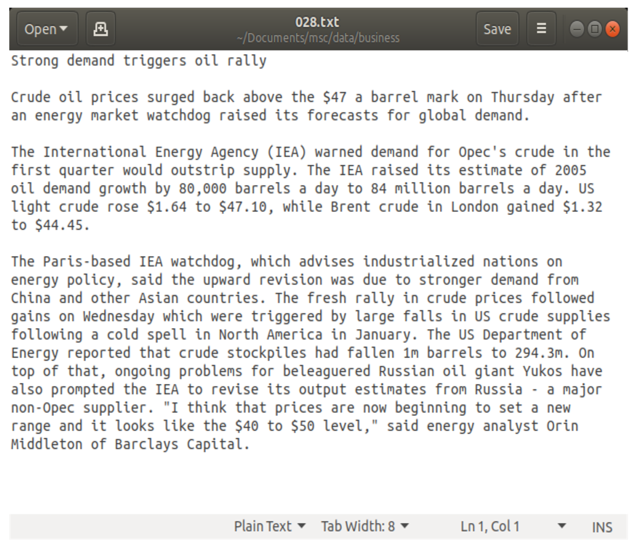
The entire calculation was performed on a dataset derived from a news database on the BBC website of the five most popular news categories from 2004 to 2005 [15]. This collection contains 2225 documents, each of which was assigned to one of the categories: “business”, “entertainment”, “politics”, “sports”, or “tech”. Each document is a separate (*.txt) text file assigned to a directory structure that defines the category membership. Pre-processing of these documents allowed us to extract 12,162 texts forming the basis for the calculations. All of the extracted texts were used in the comparison. These data are much more than the text documents due to the fact that a single document contained several unrelated messages separated by multiple newline characters. One example text document is shown in Figure 1.
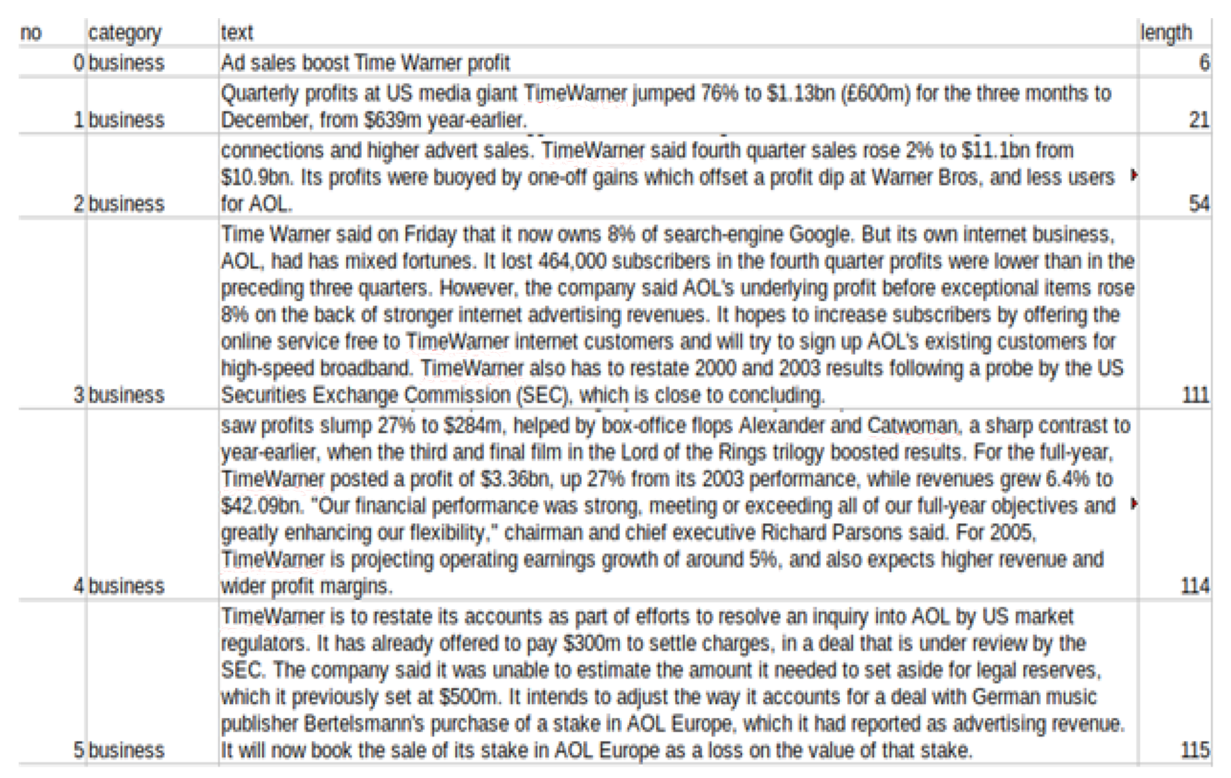
Data from all of the text files were compiled into a single *.csv file containing the following columns (Figure 2):
- no—ordinal number, allowing the unique identity of the text,
- category—single category to which the text belongs,
- text—basic data,
- length—the length of the text (it was helpful in the collection of further statistics on the texts, and also allowed the detection of initial errors in the script for dividing text documents into individual texts).
In order to better describe the structure of the texts for each category and for all texts, the following measurements were made: number of texts, mean text length (in words), median text length (in words), maximum text length (in words), and minimum text length (in words).
3.1. Aggregate Data Analysis
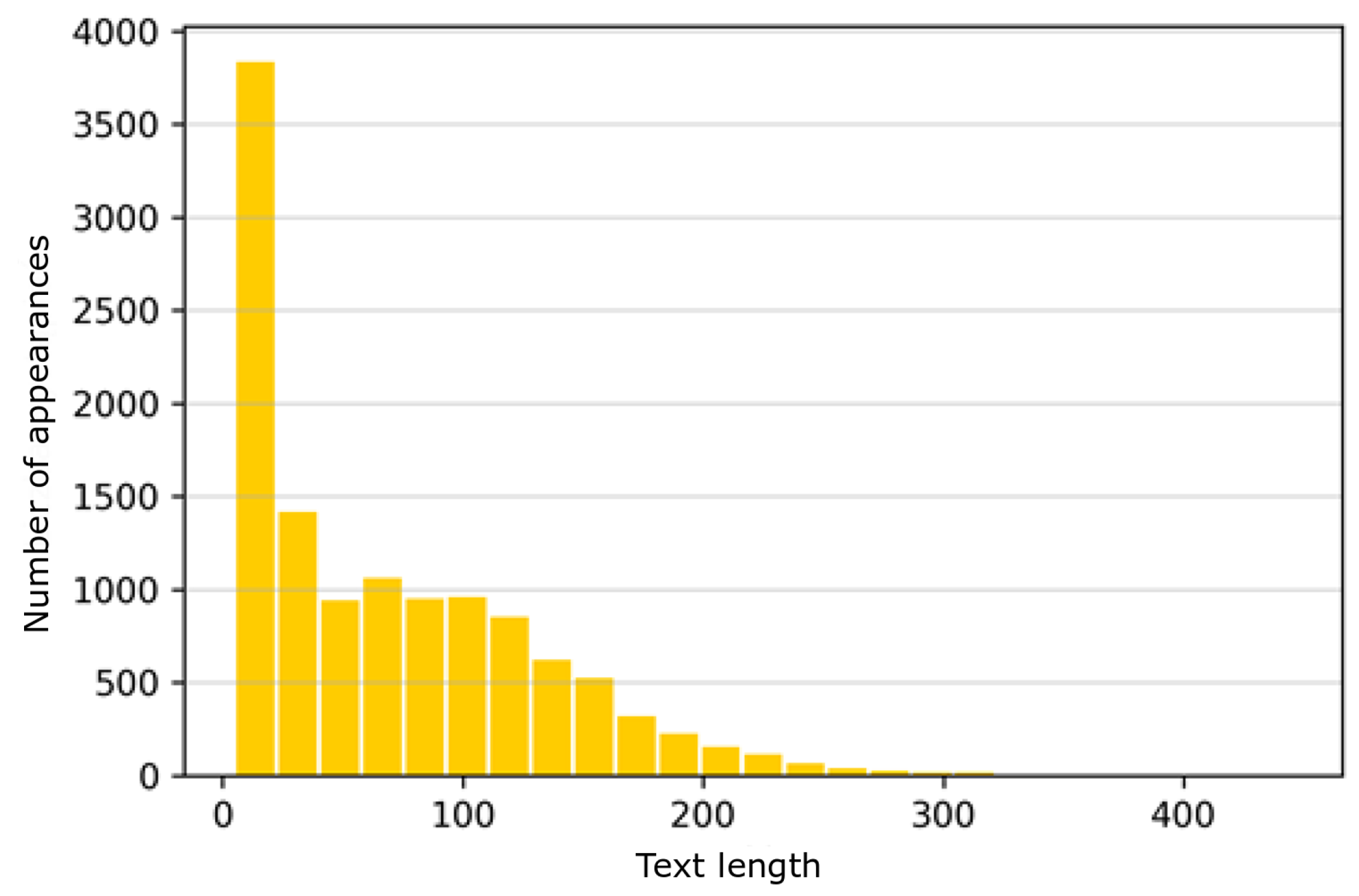
As can be seen on the histogram, the structure of text length is not homogeneous. Short texts (up to 50 words) predominate, while there are very few texts longer than 200 words. The consequence of this structure of all texts is the faster processing of data in the learning process. However, it may result in the shortest texts between categories to be hardly distinguishable.
3.2. Data Analysis for Single Categories
The data from each category were then analyzed against each other. The basic statistics by category are presented in Table 1. It shows that all categories have a similar number of texts, about 2500 texts. The dataset for the “entertainment” category is the least numerous. While the most numerous was for the “business” category. The average text length between categories varies between 62 for the “entertainment” category and 81 for the “tech” category, while the median is lower, ranging between 39 for the “sports” category and 65 for the “politics” category. The longest of the texts belongs to the “sports” category, while the shortest text for all categories is only 5 words.
All collections of texts by category have a similar structure. Most are short texts, under 50 words, while very few are second texts, over 200 words. For each category, the length distribution is similar to the summary distribution, and also the distributions are similar between categories. This makes it possible to simply conclude that the length of the texts does not affect the results because it is not a characteristic of any category of the texts. It would be different if the training set took a category with only long texts and another with only short texts. In that case, it could have a negative impact on the results and the subsequent classification of the texts, thus undermining the reliability of the research conducted.
3.3. Text Preparation
Performing the learning process on text data requires the appropriate prior preparation. Each document is transformed in the same way so that it can be represented in vector form, then placed in the appropriate analysis space. We refer to the basic operations that a text document can undergo shallow text analysis and the following transformations, performed in the following order:
- Removal of special characters—most electronic texts contain characters related to text formatting, whose removal is important for optimal processing.
- Uniform size of letters—since all text processing algorithms are case-sensitive, it is necessary to force all letters to be the same size.
- Remove punctuation and quotation marks—punctuation and quotation marks in sentences play a communicative role. In automatic natural language analysis, it is necessary to decide whether the value added by punctuation is large enough. Leaving punctuation unmodified increases the dataset size to be processed and further complicates the computation. In the case of classifying the topic of an utterance, it is not so important. It is different when we analyze the emotional coloring of an utterance (whether it is positive or negative). Then, the punctuation, especially emotional signs (exclamation marks, question marks, ellipsis), may prove crucial for the interpretation of the text.
- Remove possessive pronouns—they indicate belonging to someone or something. In the framework of automatic text analysis, especially the classification of the subject of the text, the information about affiliation is not necessary, but as in the case of punctuation marks, each case of automatic text analysis should be considered individually in terms of the usefulness of this information.
- Lemmatization—is the process by which we replace words with their base form or lemma. The use of lemmatization is important because the same word can take different forms, each of which carries the same information, and unfortunately, the machine treats them as completely different words. In the case of English, we lemmatize only the verbs. In order to determine what part of speech a given word is and what its lemma is, dictionary methods are most often used. They consist in storing in memory the entire dictionary for a given language. In practice, dictionary methods are often imperfect and may not contain a complete dictionary due to the high dynamics of language change; this may be especially important when analyzing informal or youth texts.
- Removal of “stop words"—stop words are words that occur relatively often in the studied set of documents and, at the same time, are irrelevant because they do not carry information. For each language, there are commonly available sets of such words. Removing them from the text allows the statistical models needed for classification to work correctly but may completely change the meaning of the text.
The step of removing the “stop words” in preprocessing the text can be as follows:
- stop_words = list(stopwords.words(’english’))
- df[’text_6’] = df[’text_5’]
- for stop_word in stop_words:
- regex_stopword = r"\b" + stop_word + r"\b"
- df[’text_6’] = df[’text_6’].str.replace(regex_stopword, ’’)
The last step is to re-save the result of all performed operations to *.csv files—the first file contains the texts together with all data preprocessing steps, while the second contains only category information, original text, and the result of all processing.
3.4. Vectorization
The implementation of vectorization methods to compare classification results used the gensim library of Python, which provides ready-made Word2Vec and Doc2Vec models. In order to create a CBOW model, the Word2Vec method is used as follows:
- model = Word2Vec(documents, vector_size=100, window=5,
- min_count=2, workers=8, sg=0)
The parameters successively accepted by the method that creates the model are:
- document, which is the object containing the tagged texts,
- vector_size, which is the size of the resulting vectors, in this case, as in the other methods, it is 100,
- window, which is the maximum distance between the current word and the predicted word in the sentence, in this case, 5,
- min_count, a number deciding which words will be ignored when creating vectors—if a given word occurs less than the given number, it will not be taken into account during vectorization,
- workers, or the number of auxiliary threads used in training the model, this value should be adjusted to the number of processors on which the learning process is performed.
The unique parameter for the Word2Vec method is the sg parameter—it is the parameter that determines whether the CBOW or Skip-gram method will be used. When it is 0, it is CBOW, and when it is 1, it is Skip-gram.
The vectors created in this way for words should be converted into features of texts allowing their fundamental classification. The simplest way is to average the word vectors for all words in the text. For this purpose, we built a transformer initialized with a word:
- class MeanEmbeddingVectorizer(object):
- def __init__(self, word2vec):
- self.word2vec = word2vec
- # if a text is empty we should return a vector
- of zeros
- # with the same dimensionality as all the other
- vectors
- self.dim = len(word2vec.itervalues().next())
- def fit(self, X, y):
- return self
- def transform(self, X):
- return np.array([
- np.mean([self.word2vec[w] for w in words if w in
- self.word2vec]
- or [np.zeros(self.dim)], axis=0)
- for words in X
- ])
A whole-text-based method, DM-PV, or Doc2Vec, was used for comparison. The process of creating this model is analogous to the process of creating the Word2Vec model as follows:
- model = Doc2Vec(documents, vector_size=100, window=5,
- min_count=2, workers=8)
Each model was learned in exactly the same way, for a predefined number of epochs max_epochs equal to 200.
3.5. Data Split
For adequate validation, it was necessary to split the dataset according to cross-validation recommendations. A 10-fold cross validation was used. The script to split the dataset into training and testing looks as follows:
- k = 10
- cv = model_selection.StratifiedKFold(n_splits=k)
- fold = 0
- for train, test in cv.split(documents):
- print "Fold %i (%i w TS, %i w VS)" % (fold, len(train),
- len(test))
- fold += 1
Initially, a constant k for k-fold cross-validation was declared, which is the target number of splits. Then the cv split object is initialized with this parameter. Finally, the loop iterates over the cv object and displays the sizes of the split sets: train and test.
3.6. Classification Task
Two methods, the k-nearest neighbors and Naive Bayesian Classifier, were used for the classification task. Both of these methods are very simple. This is very important because classification has been chosen as the determinant of the overall performance of a text mining method. More than one method was chosen to see if the trends for the selected vectorization methods were the same for different text classification methods.
The methods used for classification are from the sklearn library. The k-nearest neighbour method, where n is equal to 5, is as follows:
- #Import knearest neighbors Classifier model
- from sklearn.neighbors import KNeighborsClassifier
- #Create KNN Classifier
- knn = KNeighborsClassifier(n_neighbors=5)
The Naive Bayesian Classifier (NBC) method is as follows:
- #Import Naive Bayes Classifier
- from sklearn.naive_bayes import GaussianNB
- #Create KNN Classifier
- nbc = GaussianNB()
4. Results of Experiments and Their Analysis
The realized experiments contained 10 tests. Each of them used one of five implemented text vectorization methods in combination with one of the two text classification methods. This yielded the following test cases:
- vectorization by the CBOW method with word vector averaging for texts, classification by the k-nearest neighbors method, denoted in the results as CBOW k-NN,
- Skip-gram vectorization with word vector averaging for texts, classification by the k-nearest neighbors method, denoted in the results as Skip-gram k-NN,
- CBOW vectorization with the tf-idf method, k-nearest neighbors classification, denoted in the results as CBOW tf-idf k-NN,
- Skip-gram vectorization using the tf-idf method, k-nearest neighbors classification, denoted in the results as Skip-gram tf-idf k-NN,
- DM-PV vectorization, k-nearest neighbor classification, doc2vec k-NN,
- CBOW vectorization with word vector averaging for texts, Naive Bayesian Classifier classification, denoted as CBOW NBC in the results,
- Skip-gram vectorization with word vector averaging for texts, Naive Bayesian Classifier classification, denoted as Skip-gram NBC in the results,
- CBOW vectorization with tf-idf, Naive Bayesian Classifier, denoted as CBOW tf-idf NBC in the results,
- Skip-gram vectorization using the tf-idf method, Naive Bayesian Classifier, denoted in the results as Skip-gram tf-idf NBC,
- vectorization with the DM-PV method, Naïve Bayesian Classifier, denoted as doc2vec NBC in the results.
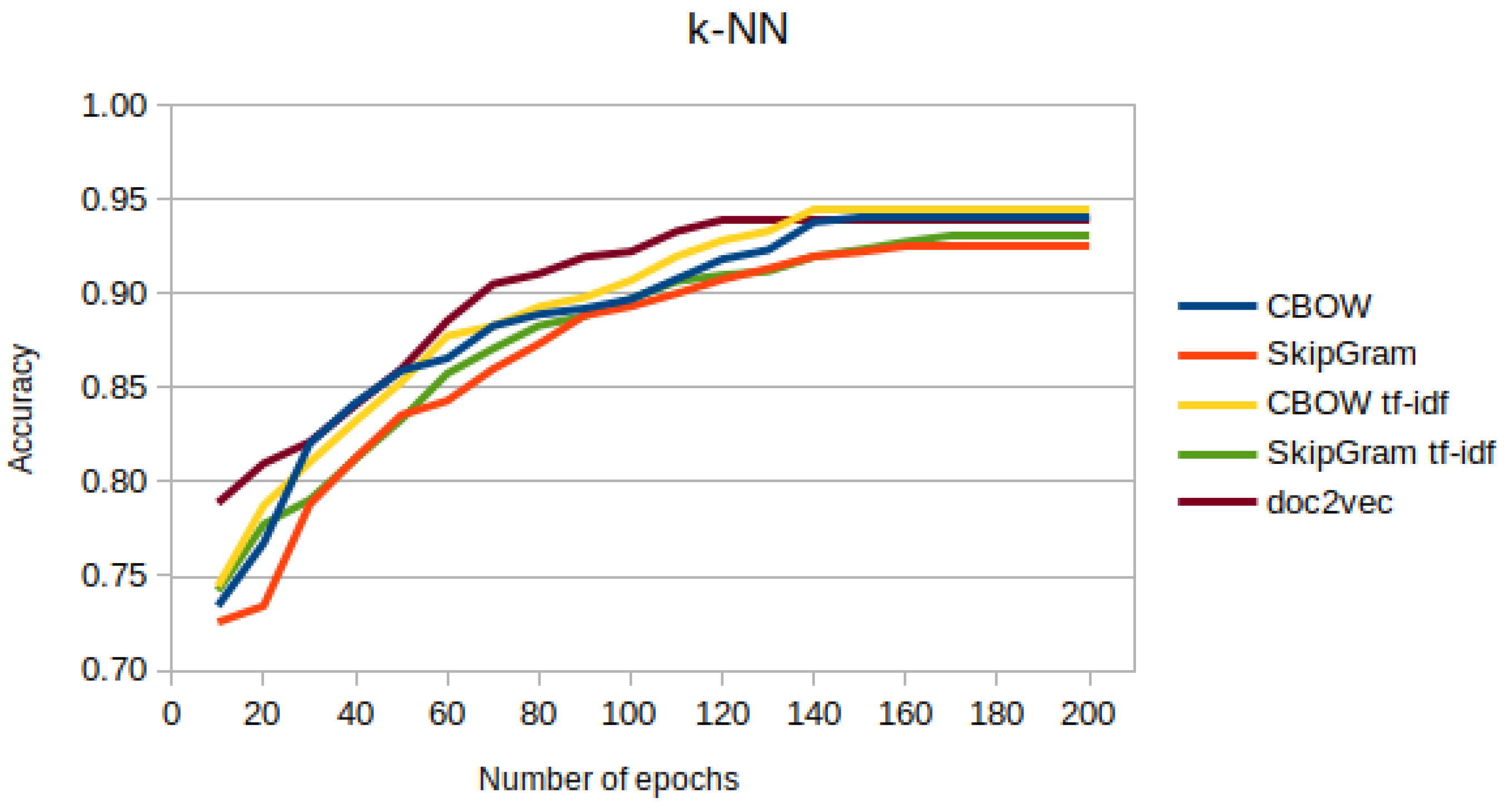
The results for the tests performed were compared under the classification method. The test results for the k-nearest neighbor method are shown in Table 2 and Table 3 and Figure 4.
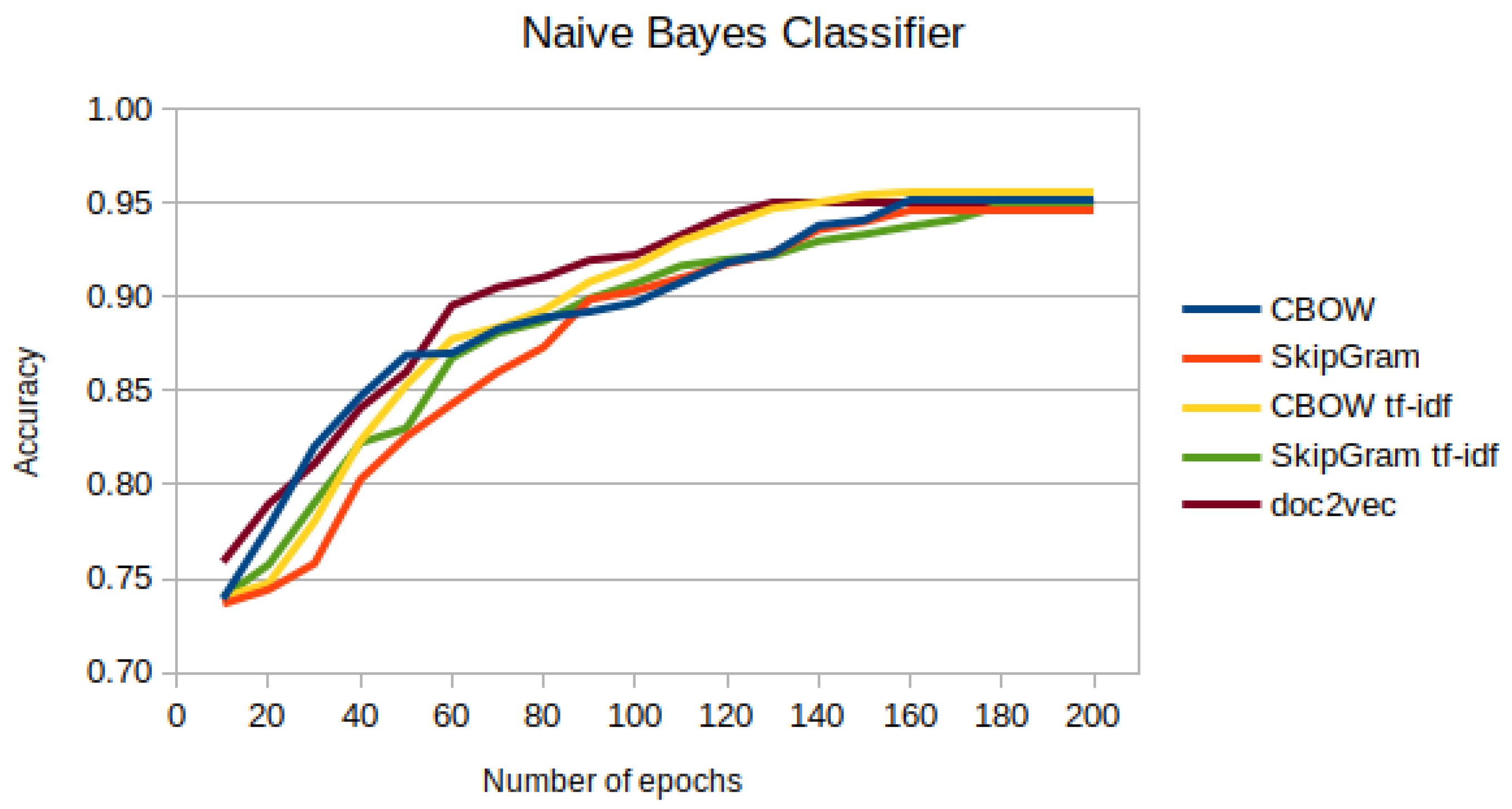
As can be seen from the data obtained, none of the methods stood out in terms of efficiency in the case studied. For the k-nearest neighbor method, the final results are in the range of [0.92; 0.95], while for the Naive Bayesian Classifier, they are in the range of [0.94; 0.96]. The results obtained using NBC show much smaller differences than the k-NN method. At the same time, it should be noted that the classification performance of this method is better than the classification via the much simpler k-NN method.
Regardless of the classification method chosen, the Continuous Bag of Words method with feature extraction using Term Frequency—Inverse Document Frequency performed best. In the case of classification with the k-NN method, an accuracy score of 0.945 was obtained, while using the Naïve Bayesian Classifier, it was 0.955.
However, for the studied case of document topic classification, the lowest performance results were obtained using the Skip-gram method when averaging the word vectors. The classification of previously vectorized text with this method using k-NN yielded a score of 0.926 while using NBC yielded a score of 0.947.
The method that took the longest time for the obtained performance result to be invariant across subsequent iterations was the Skip-gram method using tf-idf feature extraction. For the k-NN method, it was 166 epochs, while for the Bayesian classifier, it was as long as 179. This long time may be due to the complexity of the vectors obtained from this method. Despite the fact that the model is actually a mirror image of the CBOW method, it ultimately creates many more dependencies between words. These dependencies, which are often not obvious, can have a major impact on the time required to obtain invariant performance.
On the other hand, the method that needed the least number of epochs to obtain an invariant efficiency result is the Distributed Memory—Paragraphs Vectors method. It takes only 112 epochs for the k-NN method and 125 epochs for the Naive Bayesian Classifier. This short time, compared to the Skip-gram tf-idf method mentioned earlier, may be due to directly creating vectors based on whole texts rather than first creating vectors of words and then creating vectors of texts based on those vectors. This approach allows the machine to detect relationships within whole texts earlier, which are not as obvious for word-based methods. In addition, this method obtained performance results significantly higher than the other tested methods from the very beginning. Hence the relative value of the obtained performance was lower with a similar absolute result.
Another aspect worth noting is the course of effectiveness values depending on the epoch. Irrespective of the method of text classification, the course of these functions was similar. In the early epochs, the accuracy values increase faster, while already around the 100th epoch, the effectiveness differences in subsequent epochs are not so large. Interestingly, the method with the worst performance also starts with the lowest score. However, what the initial classification score is is in no way an indicator of whether the method will work. This can be seen in the CBOW method. In the initial epochs, the accuracy score using this method is second-worst, while after getting its best accuracy score, it is the second-best. Consequently, this means that it is impossible to unambiguously decide whether the method will work in the case under study (cannot decide on the effectiveness of the method by analyzing the initial results).
It is also worth emphasizing the fact that all methods of text vectorization gave a similar course of the accuracy function in subsequent epochs regardless of the chosen method of classification.
5. Comparison with Results of Studies Available in the Literature
Exactly the same results are not available in the literature for all the methods addressed in this paper. Therefore, the comparison made was focused on the works described in [16,17,18].
The obtained results of classification accuracy are consistent with those available in the literature. The effectiveness of the methods tested in [16] ranges from 0.8 to 0.95. A comparison of the obtained effectiveness for the analysis of news texts from the [16] and our work is given in Table 6.
As can be seen, the efficiency value is practically the same. The number of epochs needed to train the CBOW method is also similar. In the case of the Skip-gram method, the number of epochs is even higher than the research conducted in this paper. This is an additional confirmation that the Skip-gram method, due to the creation of complex vectors, needs more time to achieve satisfactory performance.
In addition, the authors of [16] have included graphs showing the variation of accuracy depending on the epoch. These results are similar to those obtained in our work, except that in [16], as early as around epoch 50, the effectiveness is close to the final effectiveness, while in the case of our work, only for epoch 130, the results were close. This behavior may be due to the choice of the test set for the methods. The more difficult it is, the more time will be needed to train the same effective method.
In contrast, the results in [17] are different. The summary includes a comparison of a class of texts represented by many documents and by few documents. A comparison of these data with the present work is shown in Table 7.
The largest discrepancy is seen here for the doc2vec method. The authors of [17] point out that the behavior of this method in the tests they performed is different from those available in [13]. This result may be influenced by the authors’ use of Chinese language texts in the context of public financial documents for classification.
The same methods in many publications have been tested on different datasets, and it is the selection of the dataset that determines their effectiveness. For comparison, in [19], CBOW was compared for several datasets and the respective effectiveness was 61.8% for MR [19], 77.9% for SST [20], and 87.1% for IMDB [21]. For the same datasets, tests were also conducted for the Skip-gram method; the corresponding MR was 63.5%, SST was 77.3%, and IMDB was 89.1%. Which clearly allows us to conclude that it is the complexity of the data to be created and then classified that determines the effectiveness of the method. Hence, different methods for the same datasets have similar effectiveness in terms of values. It is also worth noting that the effectiveness of the Skip-gram method within the study [18] is higher than CBOW, contrary to what came out in this study.
6. Discussion and Conclusions
The result of our work is a summary of text vectorization methods in the context of the obtained classification performance for two word-based methods (Continuous Bag of Words, Skip-gram) in two variants of feature extraction (by averaging and by the tf-idf method) and for one method based on the whole document (Distributed Memory Paragraph Vectors). This summary has been prepared for two very simple classification methods (k-nearest neighbor method and Naive Bayesian Classifier). These results give grounds to consider the choice of the text vectorization method as a factor influencing the classification performance.
The obtained results can easily be considered reliable. All experiments were performed on a relatively large dataset (more than 12 thousand texts with an average length of about 70 words). This means that the size of the training set had no negative impact on the performance of the vectorization methods. In addition, the variety of categories for which it was possible to perform classification within a single text type (web news content) allowed for a good description of the relationship between the vectorization methods and classification performance.
It is also worth emphasizing the fact that the course of the effectiveness function in successive epochs is independent of the classification method. As was already mentioned, this independence allows the choice of the method of text vectorization to be considered as an important factor determining the accuracy of the classification. Going further, it allows us to hypothesize that the creation of a text vectorization method combining the advantages of currently known methods or types of methods could further increase the classification efficiency. Which, as a consequence, would mean an increase in the efficiency and accuracy of the processing or understanding of texts by machines. The combination of these issues, together with methods that analyze speech and create their transcriptions, offers great opportunities for the development of AI.
Worth noting is the relationship between learning speed and the type of text vectorization method. Word-based methods are slower than those based on vectorization of the entire text. At the same time, both types of vectorization methods produce similar classification performance results. It is worth considering a combination of word-based methods with simultaneous global context (relative to all words in the language) and whole-text-based methods with local context (only the texts on which the vectorization methods have been trained). This combination could allow for even better results while optimizing the number of learning epochs. Research is already underway on how text vectors should be created to best allow them to be represented. One example of a new approach to text vectorization is the use of an attention mechanism in the learning process [22].
Regarding some limitations of this study, among the most important are:
- comparison of only word and sentence embeddings methods, future research should also focus on other methods, such as those based on transformers architecture,
- the use of classification as a determinant of the effectiveness of the methods—there are many other methods to test the effectiveness of the methods, for example, by comparing word vectors or similarity between words, but in this study, classification was deliberately chosen,
- using the classification of only the topics of texts—instead, it is worth considering options more difficult than topic recognition, such as the classification of sentiment or emotion in texts,
- only one dataset was used to test the methods—within topic recognition, it is possible to conduct tests on many other datasets, including those whose structure is more difficult of texts are much longer,
- testing only for English—in English the research on NLP issues is the most advanced. Therefore, the results of the methods may be the best in this language, it is worth analyzing the vectorization methods in comparison with other languages in the future, also from other language groups, such as Arabic or Chinese.
To conclude, it can be emphasized that the current implementations of text vectorization methods achieve similar efficiency results regardless of the method chosen. All methods achieved efficiencies above 90%, which, for the current natural language processing applications, such as spam filtering or detecting offensive comments on the Internet, is more than sufficient. Hence, further research and the optimization of methods used within NLP should focus on the development of artificial intelligence and human imitation in the understanding of written and spoken text.
The conducted research allows for further development of issues related to the creation of vector spaces in natural language processing:
- Classification of texts not only in terms of the topic of speech but also other factors, such as emotional color. Each type of classification poses new challenges for vectorization methods, such as finding other characteristics of the same texts classified first in terms of topic and then in terms of emotional color.
- Analysis of texts other than Internet news. Statements from colloquial, official, and scientific language are characterized by different phrases, often also by a different structure of the utterance. At present, we do not know a method that would allow for the simultaneous classification of texts of different types. Hence, it is worth verifying whether the use of existing methods to classify different types of texts at the same time will be effective. Another option is to try to create a method that can cope with the classification of these kinds of texts.
Author Contributions
Conceptualization, U.K. and J.O.-M.; methodology, U.K. and J.O.-M.; validation, A.P.-M. and J.O.-M.; formal analysis, U.K., A.P.-M., and J.O.-M.; investigation, U.K.; resources, U.K.; data curation, U.K.; writing—original draft preparation, U.K., A.P.-M., and J.O.-M.; writing—review and editing, A.P.-M.; visualization, A.P.-M. All authors have read and agreed to the published version of the manuscript.
Funding
This research received no external funding.
Institutional Review Board Statement
Not applicable.
Informed Consent Statement
Not applicable.
Conflicts of Interest
The authors declare no conflict of interest.
References
- Tixier, A.J.-P.; Hallowell, M.R.; Rajagopalan, B.; Bowman, D. Automated content analysis for construction safety: A natural language processing system to extract precursors and outcomes from unstructured injury reports. Autom. Constr. 2016, 62, 45–56. [Google Scholar] [CrossRef] [Green Version]
- Zou, Y.; Kiviniemi, A.; Jones, S.W. Retrieving similar cases for construction project risk management using Natural Language Processing techniques. Autom. Constr. 2017, 80, 66–76. [Google Scholar] [CrossRef]
- Jain, A.; Kulkarni, G.; Shah, V. Natural Language Processing. Int. J. Comput. Sci. Eng. 2018, 6, 161–167. [Google Scholar] [CrossRef] [Green Version]
- Khurana, D.; Koli, A.; Khatter, K.; Singh, S. Natural Language Processing: State of The Art. Current Trends and Challenges. arXiv 2017, arXiv:1708.05148. [Google Scholar]
- Mikolov, T.; Sutskever, I.; Chen, K.; Corrado, G.S.; Dean, J. Distributed Representations of Words and Phrases and their Compositionality. In Proceedings of the 26th International Conference on Neural Information Processing Systems, Lake Tahoe, NV, USA, 5–10 December 2013; Volume 2, pp. 3111–3119. [Google Scholar]
- Mikolov, T.; Chen, K.; Corrado, G.; Dean, J. Efficient Estimation of Word Representations in Vector Space. arXiv 2013, arXiv:1301.3781. [Google Scholar]
- Qun, L.; Weiran, X.; Jun, G. A Study on the CBOW Model’s Overfitting and Stability. In Proceedings of the International Conference on Information and Knowledge Management, Shanghai, China, 3 November 2014; pp. 9–12. [Google Scholar] [CrossRef]
- Yan, S.; Shuming, S.; Jing, L.; Haisong, Z. Directional Skip-Gram: Explicitly Distinguishing Left and Right Context for Word Embeddings. In Proceedings of the 2018 Conference of the North American Chapter of the Association for Computational Linguistics: Human Language Technologies, Volume 2 (Short Papers); Association for Computational Linguistics: New Orleans, LA, USA, 2018; pp. 175–180. [Google Scholar] [CrossRef]
- Salton, G.; Wong, A.; Yang, C.S. A vector space model for automatic indexing. Commun. ACM 1975, 18, 613–620. [Google Scholar] [CrossRef] [Green Version]
- Shahzad, Q.; Ramsha, A. Text Mining: Use of TF-IDF to Examine the Relevance of Words to Documents. Int. J. Comput. Appl. 2018, 181. [Google Scholar] [CrossRef]
- Stephen, R. Understanding Inverse Document Frequency: On Theoretical Arguments for IDF. J. Doc. 2004, 60, 503–520. [Google Scholar] [CrossRef] [Green Version]
- Havrlanta, L.; Kreinovich, V. A Simple Probabilistic Explanation of Term Frequency-InverseDocument Frequency (tf-idf ) Heuristic (and Variations Motivatedby This Explanation). Int. J. Gen. Syst. 2015, 46, 27–36. [Google Scholar] [CrossRef] [Green Version]
- Le, Q.V.; Mikolov, T. Distributed Representations of Sentences and Documents. arXiv 2014, arXiv:1405.4053. [Google Scholar]
- Douzi, S.; Amar, M.; El Ouahidi, B.; Laanaya, H. Towards A new Spam Filter Based on PV-DM (Paragraph Vector-Distributed Memory Approach). Procedia Comput. Sci. 2017, 110, 486–491. [Google Scholar] [CrossRef]
- Green, D.; Cunningham, P. Practical Solutions to the Problem of Diagonal Dominance in Kernel Document Clustering. In Proceedings of the ICML 2006, Pittsburgh, PA, USA, 25–29 June 2006. [Google Scholar]
- Jang, B.; Kim, I.; Kim, J. Word2vec convolutional neural networks for classification of news articles and tweets. PLoS ONE 2019, 14, e0220976. [Google Scholar] [CrossRef] [Green Version]
- Wang, Y.; Zhou, Z.; Jin, S.; Liu, D.; Lu, M. Comparisons and Selections of Features and Classifiers for Short Text Classification. Iop Conf. Ser. Mater. Sci. Eng. 2017, 261, 012018. [Google Scholar] [CrossRef] [Green Version]
- Lei, X.; Cai, Y.; Xu, J.; Ren, D.; Li, Q.; Leung, H.-F. Incorporating Task-Oriented Representation in Text Classification. Available online: https://openreview.net/forum?id=LYknk8R-Bht (accessed on 2 October 2021).
- Database for Sentiment Analysis. Available online: https://0-www-cs-jhu-edu.brum.beds.ac.uk/mdredze/datasets/sentiment/unprocessed.tar.gz (accessed on 2 November 2021).
- Movie review data for Sentiment Analysis. Available online: https://www.cs.cornell.edu/people/pabo/movie-review-data/ (accessed on 3 November 2021).
- Deeply Moving: Deep Learning for Sentiment Analysis. Available online: http://nlp.stanford.edu/sentiment (accessed on 2 November 2021).
- Linden, J.; Forsstrom, S.; Zhang, T. Evaluating Combinations of Classification Algorithms and Paragraph Vectors for News Article Classification. In Proceedings of the 2018 Federated Conference on Computer Science and Information Systems, Poznań, Poland, 9–12 September 2018; pp. 489–495. [Google Scholar] [CrossRef] [Green Version]
Figure 1.
Example of the initial text file used for the calculation.

Figure 2.
Extract of *.csv file obtained from individual text files used for the calculation.

Figure 3.
Summary statistics of data in studied texts—length of texts for all categories.

Figure 4.
Accuracy of k-NN classification for selected text vectorization methods by epoch.

Figure 5.
Accuracy of Naive Bayesian Classifier classification for selected text vectorization methods by epoch.
Figure 5.
Accuracy of Naive Bayesian Classifier classification for selected text vectorization methods by epoch.


Table 1.
Summary statistics of the data in all of the studied texts by category.
| All | Business | Entertainment | Politics | Sport | Tech | |
|---|---|---|---|---|---|---|
| Number of texts | 12,162 | 2624 | 2053 | 2538 | 2459 | 2488 |
| Average length | 70 | 64 | 62 | 73 | 69 | 81 |
| Quarterly deviation | 45.5 | 42 | 39 | 45.5 | 49.5 | 54 |
| Median length | 56 | 54 | 53 | 65 | 39 | 60 |
| Maximum length | 445 | 283 | 273 | 292 | 445 | 423 |
| Minimum length | 5 | 5 | 5 | 5 | 5 | 5 |
Table 2.
Accuracy of k-NN classification for different vectorization methods.
| Accuracy | Epoch | |
|---|---|---|
| CBOW k-NN | 0.941 | 144 |
| Skip-gram k-NN | 0.926 | 152 |
| CBOW tf-idf k-NN | 0.945 | 137 |
| Skip-gram tf-idf k-NN | 0.931 | 166 |
| Dov2vec k-NN | 0.939 | 112 |
Table 3.
Precision, recall, and F1 scores for all vectorization methods with k-NN classification by specific topics.
Table 3.
Precision, recall, and F1 scores for all vectorization methods with k-NN classification by specific topics.
| CBOW | SkipGram | CBOW TF-TDF | SkipGram TF-TDF | Doc2vec | |
|---|---|---|---|---|---|
| Business precision | 0.96 | 1 | 0.95 | 0.92 | 0.95 |
| Business recall | 0.94 | 0.93 | 0.95 | 0.93 | 0.94 |
| Business F1 | 0.95 | 0.96 | 0.95 | 0.93 | 0.94 |
| Entertainment precision | 0.86 | 0.87 | 0.93 | 0.9 | 0.91 |
| Entertainment recall | 0.94 | 0.93 | 0.94 | 0.93 | 0.94 |
| Entertainment F1 | 0.9 | 0.9 | 0.94 | 0.91 | 0.92 |
| Politics precision | 0.96 | 0.92 | 0.96 | 0.97 | 0.96 |
| Politics recall | 0.94 | 0.93 | 0.94 | 0.93 | 0.94 |
| Politics F1 | 0.95 | 0.92 | 0.95 | 0.95 | 0.95 |
| Sport precision | 0.96 | 0.92 | 0.94 | 0.94 | 0.94 |
| Sport recall | 0.94 | 0.93 | 0.94 | 0.93 | 0.94 |
| Sport F1 | 0.95 | 0.92 | 0.94 | 0.93 | 0.94 |
| Tech precision | 0.96 | 0.92 | 0.95 | 0.92 | 0.94 |
| Tech recall | 0.94 | 0.93 | 0.94 | 0.93 | 0.94 |
| Tech F1 | 0.95 | 0.92 | 0.95 | 0.93 | 0.94 |
Table 4.
Accuracy of Naive Bayesian Classifier classification for different vectorization methods.
| Accuracy | Epoch | |
|---|---|---|
| CBOW NBC | 0.951 | 153 |
| Skip-gram NBC | 0.947 | 157 |
| CBOW tf-idf NBC | 0.955 | 146 |
| Skip-gram tf-idf k-NN | 0.949 | 179 |
| Dov2vec k-NN | 0.950 | 125 |
Table 5.
Precision, recall, and F1 scores for all vectorization methods with Naive Bayesian Classifier classification by specific topics.
Table 5.
Precision, recall, and F1 scores for all vectorization methods with Naive Bayesian Classifier classification by specific topics.
| CBOW | SkipGram | CBOW TF-TDF | SkipGram TF-TDF | Doc2vec | |
|---|---|---|---|---|---|
| Business precision | 0.95 | 0.98 | 0.9 | 0.97 | 0.91 |
| Business recall | 0.97 | 0.91 | 0.9 | 0.9 | 0.9 |
| Business F1 | 0.96 | 0.94 | 0.9 | 0.94 | 0.91 |
| Entertainment precision | 0.99 | 0.91 | 0.93 | 0.93 | 0.95 |
| Entertainment recall | 0.97 | 0.97 | 0.95 | 0.96 | 0.99 |
| Entertainment F1 | 0.98 | 0.94 | 0.94 | 0.95 | 0.97 |
| Politics precision | 0.93 | 0.96 | 0.99 | 0.93 | 0.97 |
| Politics recall | 0.84 | 0.97 | 0.97 | 0.96 | 0.96 |
| Politics F1 | 0.89 | 0.96 | 0.98 | 0.94 | 0.97 |
| Sport precision | 0.97 | 0.94 | 0.97 | 0.97 | 0.96 |
| Sport recall | 0.99 | 0.95 | 0.98 | 0.96 | 0.96 |
| Sport F1 | 0.98 | 0.95 | 0.97 | 0.96 | 0.96 |
| Tech precision | 0.93 | 0.94 | 0.98 | 0.95 | 0.95 |
| Tech recall | 0.99 | 0.95 | 0.98 | 0.97 | 0.95 |
| Tech F1 | 0.96 | 0.94 | 0.98 | 0.96 | 0.95 |
Table 6.
Comparison of classification performance results for CBOW and Skip-gram methods with the work [16].
Table 6.
Comparison of classification performance results for CBOW and Skip-gram methods with the work [16].
| Effectiveness [16] | Epoch [16] | Effectiveness | Epoch | |
|---|---|---|---|---|
| CBOW | 0.9341 | 137 | 0.941 | 144 |
| Skip-gram | 0.9147 | 197 | 0.926 | 152 |
Table 7.
Comparison of classification performance results for CBOW, doc2vec and tf-idf methods with the work [17].
Publisher’s Note: MDPI stays neutral with regard to jurisdictional claims in published maps and institutional affiliations. |
© 2022 by the authors. Licensee MDPI, Basel, Switzerland. This article is an open access article distributed under the terms and conditions of the Creative Commons Attribution (CC BY) license (https://creativecommons.org/licenses/by/4.0/).
Share and Cite
MDPI and ACS Style
Krzeszewska, U.; Poniszewska-Marańda, A.; Ochelska-Mierzejewska, J. Systematic Comparison of Vectorization Methods in Classification Context. Appl. Sci. 2022, 12, 5119. https://0-doi-org.brum.beds.ac.uk/10.3390/app12105119
AMA Style
Krzeszewska U, Poniszewska-Marańda A, Ochelska-Mierzejewska J. Systematic Comparison of Vectorization Methods in Classification Context. Applied Sciences. 2022; 12(10):5119. https://0-doi-org.brum.beds.ac.uk/10.3390/app12105119
Chicago/Turabian StyleKrzeszewska, Urszula, Aneta Poniszewska-Marańda, and Joanna Ochelska-Mierzejewska. 2022. "Systematic Comparison of Vectorization Methods in Classification Context" Applied Sciences 12, no. 10: 5119. https://0-doi-org.brum.beds.ac.uk/10.3390/app12105119
Note that from the first issue of 2016, this journal uses article numbers instead of page numbers. See further details here.