
Wind Field Characteristics of Complex Terrain Based on Experimental and Numerical Investigation


1
School of Civil Engineering, Central South University, Changsha 410075, China
2
Hunan Provincial Key Laboratory for Disaster Prevention and Mitigation of Rail Transit Engineering Structures, Changsha 410075, China
3
State Key Laboratory of Mechanical Behavior and System Safety of Traffic Engineering Structures, Shijiazhuang Tiedao University, Shijiazhuang 050043, China
*
Author to whom correspondence should be addressed.
Appl. Sci. 2022, 12(10), 5124; https://0-doi-org.brum.beds.ac.uk/10.3390/app12105124
Submission received: 25 April 2022
/
Revised: 16 May 2022
/
Accepted: 17 May 2022
/
Published: 19 May 2022
(This article belongs to the Special Issue Advances in Computational Fluid Dynamics: Methods and Applications)
Abstract
:Featured Application
This article analyzes the wind characteristics of different terrain regions by numerical simulation and wind tunnel test, and the relevant research results can provide reference for wind farm site selection.
Abstract
With the intensification of energy consumption, how to make rational and efficient use of wind energy has been studied all over the world. The construction of facilities to obtain wind energy requires an accurate assessment of the wind characteristics of the local terrain. In order to study the wind characteristics on an island in Southeast China, a 1:1300 terrain model is established, and the characteristics of mean wind and fluctuating wind are studied by numerical simulation and wind tunnel test. The results show that wind speed is affected by the incoming wind direction and local terrain. Wind speed on windward slopes and flat areas with no obstructions is higher, and wind speed on leeward slopes and valleys is lower. Then, the wind attack angle of each measuring point is mainly in the range of −10°~10°, which is much higher than that in flat areas. The positive and negative wind attack angles are controlled by the incoming wind direction, and the size is closely related to the local terrain. As for pulsation characteristics, the disturbance of the inflow determines the turbulence intensity. The incoming wind direction mainly affects the turbulence intensity on the hillside, while the turbulence intensity in the valley and flat area is controlled by the local terrain. In addition, the fluctuating wind speed power spectra on the island is more consistent with the von Karman spectrum, which is quite different from the Kaimal spectrum. The bandwidth on hillsides and valleys will not change with the change in inflow, but for flat areas, the bandwidth is greatly affected by the inflow direction.
1. Introduction
In recent years, renewable energy has played an important role in environmental and climate governance by relying on its environmental protection characteristics, and the proportion of wind energy as a member of renewable energy has gradually increased [1]. Wind energy has great potential in coastal islands, which can provide energy supply for local production and life. In order to obtain wind energy, it is necessary to build specific wind energy equipment, such as windmills or wind farms. In general, wind farms will be built in areas where there is a great deal of wind energy. However, these landforms often have the characteristics of high wind attack angle and increased turbulence [2]. The atmospheric boundary layer will become more complex due to the non-uniformity of the terrain. The interaction with the wind turbine will lead to more complex flow field characteristics, and even shorten the service life of the equipment [3,4]. In addition, the complex terrain has a major impact on the wind characteristics, and the load on the independent wind turbine or the wind turbine in the wind farm is determined by the terrain [5]. Considering the safety of wind turbines and other equipment, accurate prediction of wind fields is the main work.
In the early stage of wind field research, a large number of theoretical analysis models were verified by two-dimensional and three-dimensional simple Hill models [6,7]. Many scholars focused on predicting the position and size of the maximum acceleration factor [8], and later researchers developed a series of models considering roughness or other factors on the basis of the original model [9,10,11]. However, these theoretical models are often not applicable on mountains with large slopes, which will produce significant errors [12]. In this case, researchers often use numerical simulation and wind tunnel tests to explore the wind field on simple or real complex terrain.
Studying the wind field of a simple hill can better reveal the mechanism and easily verify its accuracy. Some good results can be obtained by using the Reynolds-Averaged Navier–Stokes (RANS) turbulence model to study two-dimensional or three-dimensional simple hills [13,14]. However, the simulation results of fluid separation areas such as a leeward slope will be quite different, and the results obtained by different RANS models are also very different [15,16,17]. The results obtained by the large eddy simulation (LES) model are more accurate. Iizuka, Kondo and Wan [18,19] used the LES method to simulate the air flow on a two-dimensional steep slope, and the numerical simulation results with the wind tunnel test results were compared. The comparison results show that the LES model can accurately simulate the average wind speed distribution on the two-dimensional steep slope. It is worth noting that the wake behind the mountain can be accurately simulated by LES, and the mountain flow separation areas with different smooth and rough surfaces can be given [20,21]. Liu [22] studied the average velocity distribution and turbulence characteristics of airflow passing through smooth two-dimensional mountains and three-dimensional mountains through a large eddy simulation. The results show that LES can well predict the separation point and reattachment point, which is in good agreement with the experimental results. Then they carried out the research on the flow field on the rough three-dimensional hill. Different from other studies, the research gave the three-dimensional characteristics of the wind field, and the results showed that the three-dimensional characteristics of LES were in good agreement with the wind tunnel test [23]. It was found that when the air flow passes through the two-dimensional slope, the turbulence characteristics on the leeward side of the mountain change significantly using the wind tunnel tests [24,25]. The acceleration factor of the mountain with a rough surface is greater than that of the mountain with a smooth surface at the top. In addition, it was found that the acceleration effect of the mountain is related not only to the roughness of the mountain surface, but also to the roughness near the ground in the incoming direction [26,27]. At present, most studies pay more attention to the acceleration effect of the average wind speed caused by the terrain and less attention to the torsional effect (change in wind direction angle), but the torsional effect is also of great significance to the wind load of the structure [28,29,30,31]. The average wind speed at each position of multiple continuous hills is lower than that of a single hill, and the acceleration effect of continuous hills is less than that of a single hill [32,33]. For the real terrain environment, this difference is often greater, so further research is needed on the basis of simple mountain research. Uchida and Ohya [34,35,36] used the LES method and Bert used the modified RANS model to simulate the real terrain with good accuracy. Mcauliffe and Larose [37] studied the effects of four different Reynolds numbers on the results of the wind tunnel topographic test by means of a wind tunnel test. Lange [38] found that the average wind speed, wind shear and turbulence level are very sensitive to the terrain. A small modification of the terrain will lead to changes in the results, and the characteristics of the wind field are affected by the incoming wind direction. Jubayer and Hangan [39] used the combination of numerical simulation and a wind tunnel test to simulate the wind field within 1000 km2 by the CFD method, and selected the three most unfavorable wind directions from 12 directions. Taking the obtained results as the entrance conditions of the wind tunnel test, they studied the wind field characteristics of a mountain range in Columbia, Canada.
The terrain studied in this paper is an island in Guangdong, China, which is rich in wind energy resources. Many wind farms have been built on the island, with many still being planned. As we all know, the location of a wind farm is directly related to the power generation of the wind farm. The influence of artificial cliffs at the edge of the model does not need to be considered due to the seawater around the island, which greatly improves the accuracy of the wind tunnel test and numerical simulation [40,41,42,43]. The island belongs to class A landform, but the topographic characteristics of different areas on the island are also different, so it is slightly inappropriate to summarize it with the same type. Therefore, numerical simulation and a wind tunnel test are used to study the wind characteristics of the typical location of the island. The characteristics of the wind field are analyzed and discussed, which may provide a reference for the siting of wind farms and wind field research.
2. Numerical Method
2.1. Turbulence Model
LES is a turbulence model developed rapidly in recent years. After averaging the Navier–Stokes equations (N–S equation) in a small space domain, it filters out the small-scale vortices and derives the equation satisfied by the large-scale vortices, then simulates the influence of small vortices through the sub grid scale model.
The N–S equation of instantaneous quantity in each direction after filtering can be expressed as follows [22]
where is the filtered velocity; is the pressure; is the density of air; and are time and Cartesian coordinates, respectively; is the subgrid scale stress.
The above equation is an open equation. In order to solve it, the Smagorinsky eddy viscosity model is adopted in this paper. By assuming that the generation and consumption of energy are balanced, the relationship between subgrid stress and eddy viscosity is
where ; is the equilibrium component; ; is subgrid eddy viscosity coefficient and can be expressed as
where is the Smagorinsky constant; is the filtering scale; .
2.2. Basic Information of the Terrain
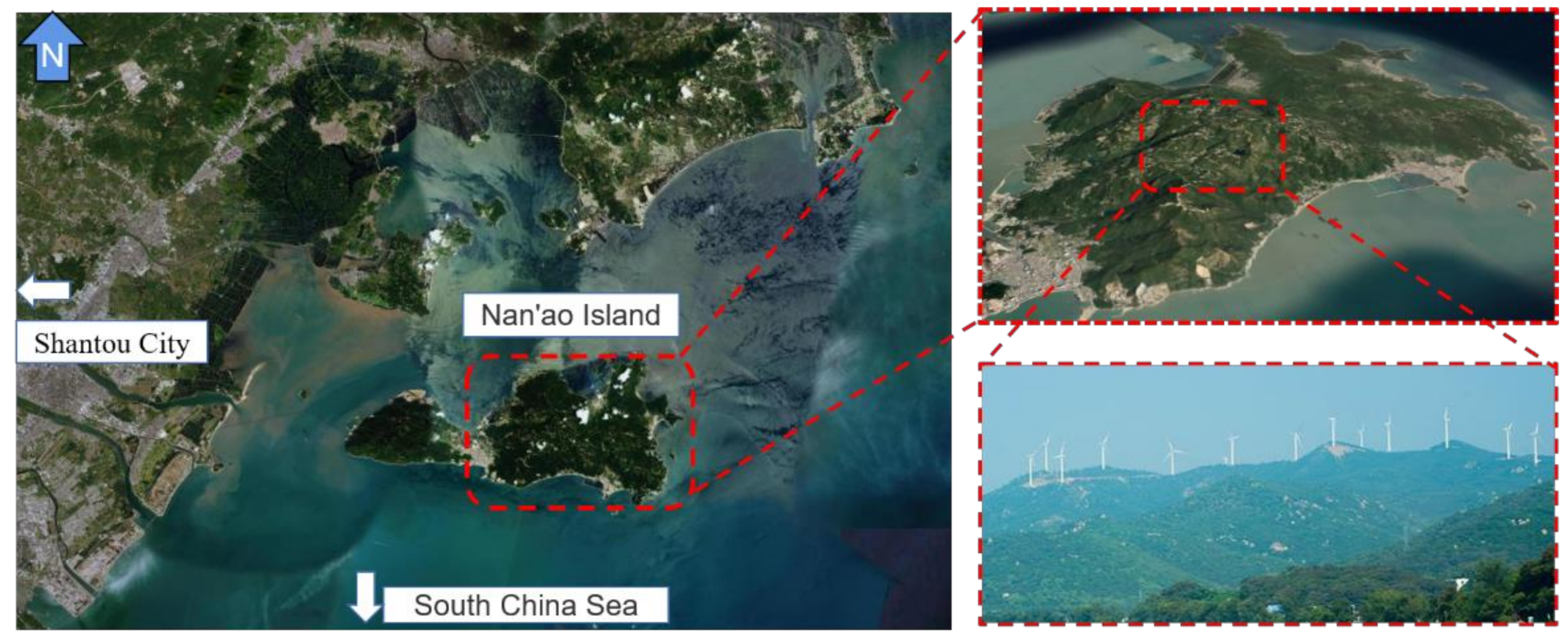
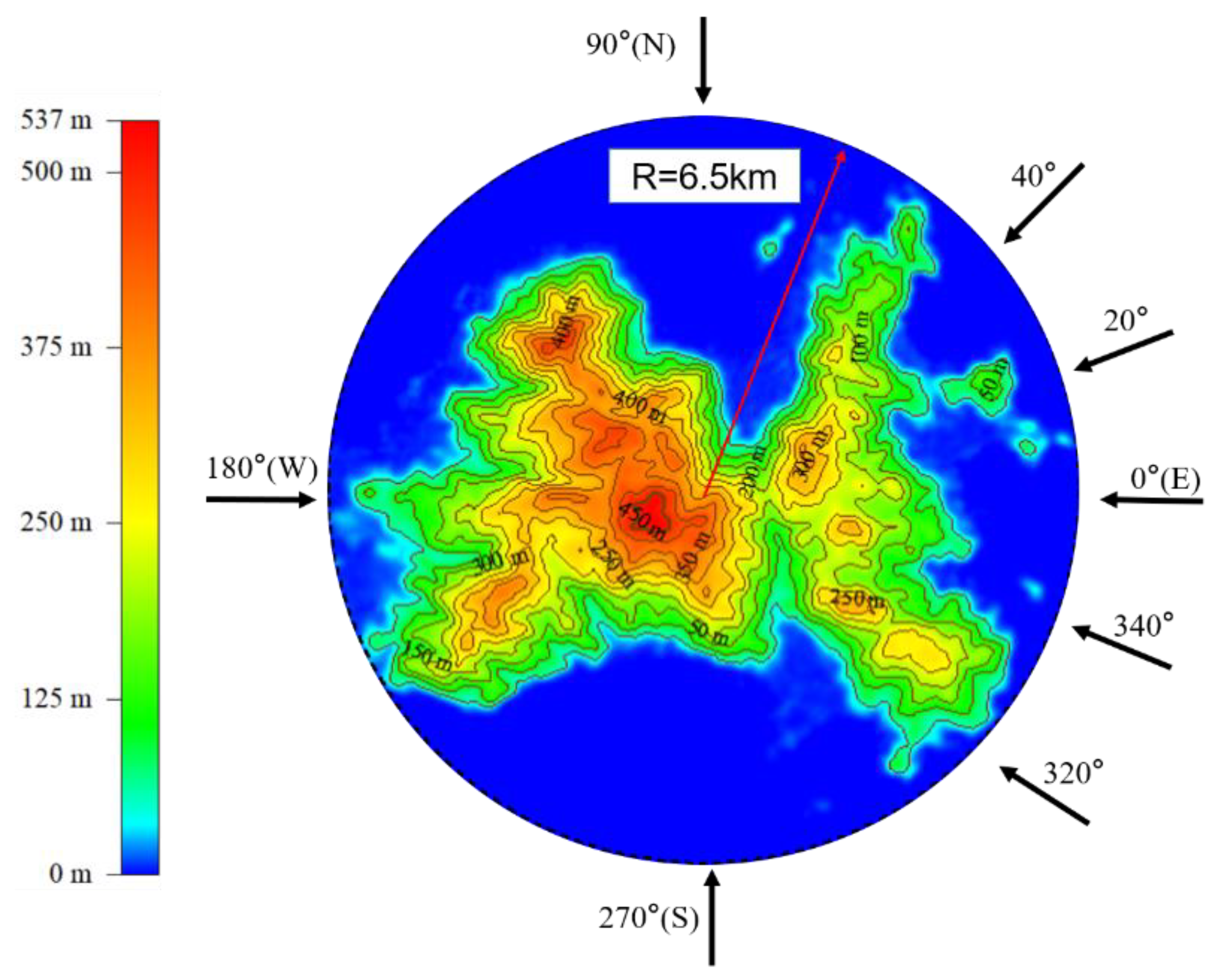
The terrain of the study is the main island of Nan’ao Island, located off the southeast coast of China. The overall terrain of the island gradually decreases from west to East, with steep mountains and sparse vegetation. The landform is dominated by high and low hills, accounting for 90% of the area of the whole island. The wind condition in Nan’ao Island is among the best in the world, with an annual average wind speed of 8.54 m/s and an effective wind speed of more than 7000 h. According to incomplete statistics, 218 wind turbines have been installed on Nan’ao Island at present, and more wind farms will be built in the future. Figure 1 shows a satellite view of the geographical location of the area.
2.3. Numerical Model
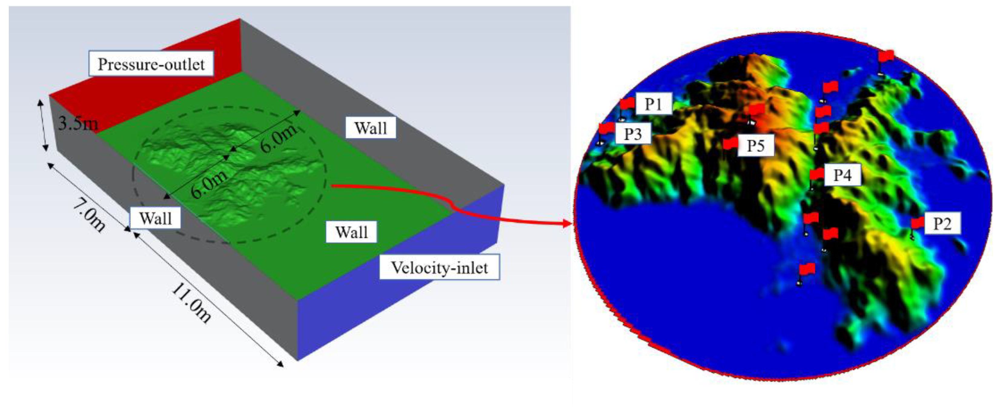
The terrain area with a diameter of 13 km is selected to establish the island terrain model. The scale of the model is 1:1300 due to the low altitude of the island. At this scale, the diameter of the island model is 10 m, and the calculation domain is consistent with the size of the low-speed wind tunnel of Central South University: 18 m long, 12 m wide and 3.5 m high. The bottom of the terrain model is sea level (0 m), so there is no need to add transition segments at the terrain boundary. The inlet boundary condition adopts velocity inlet, and the outlet boundary condition adopts pressure outlet. The top surface, bottom surface and side surfaces of the computational domain adopt non-slip wall boundary. The distance from the center of the island terrain model to both sides is 6.0 m, and the distances from the entrance and exit are 7.0 m and 11.0 m, respectively. The wind speed was set to 8 m/s with a uniform profile.
The research purpose of this paper focuses on the comparison of wind characteristics in different regions. Because the trees on the island are low, the roughness is simplified here, and only the differences caused by topographic relief are considered. In order to comprehensively evaluate the wind resources at different locations and provide reference for wind tunnel test, monitoring points are arranged on flat land, hillside, valley and mountaintop to monitor the specific value of wind characteristics. The location of wind speed monitoring points is shown in Figure 2.
2.4. Mesh of the Computational Domain
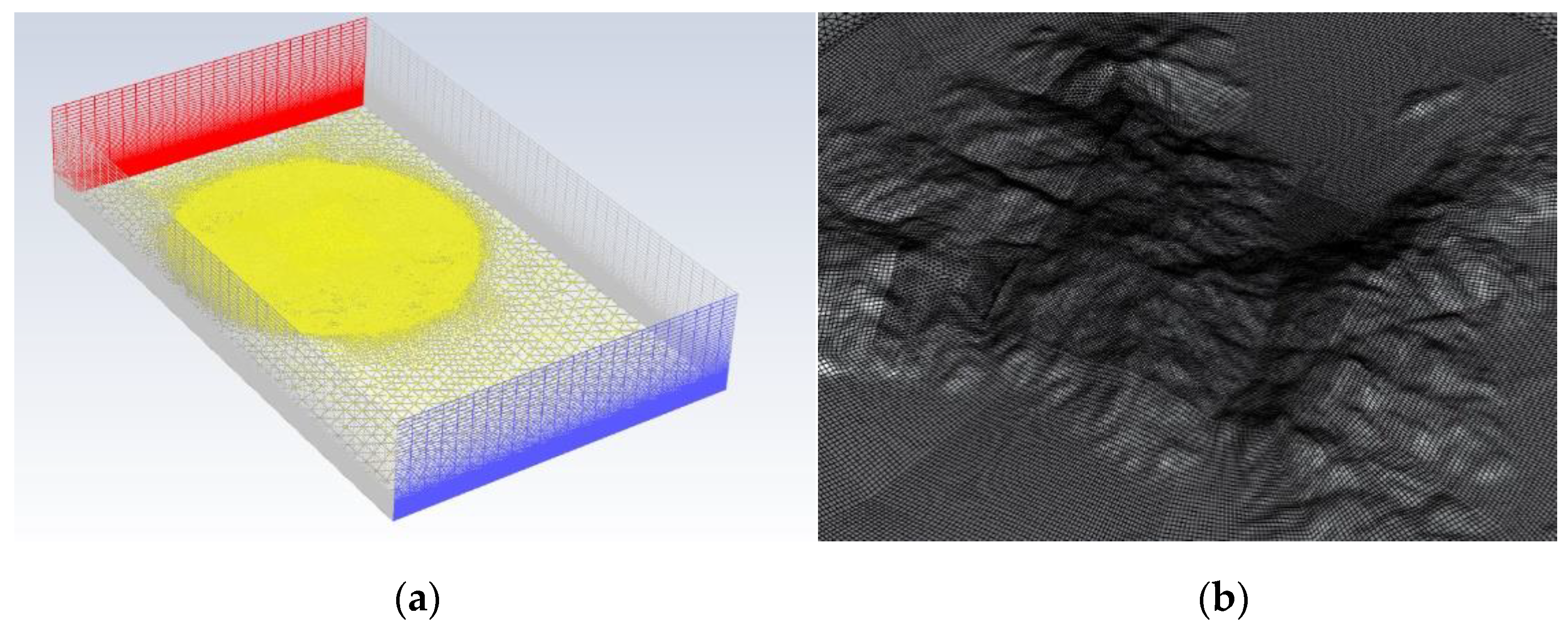
The whole model adopts the combination of structured grid and unstructured grid for grid generation. When analyzing the wind field with obvious viscous effect near the ground, it is necessary to strictly control the y+ value of the calculation grid. However, for the numerical simulation of wind field in a large area, the value of y+ has little influence on the calculation results. In order to ensure the calculation accuracy and calculation resources, the height of the first layer of grid is set to 0.0038 m and the growth rate is 1.05. It can be seen that the grid in the center of the island is small and gradually sparse outward. In order to accurately simulate the wind field on the island, some areas are encrypted. Figure 3 shows the relevant meshing. After grid independence verification, the total number of grids is 5.3 million.
In the simulation, the N–S equation is solved by simple algorithm, the pressure adopts the second-order interpolation scheme, and the momentum adopts the second-order upwind scheme. In order to meet the conditions of CFL, the time step is set to 0.0005 s and the total number of time steps is 30,000.
3. Setup of Wind Tunnel Test
3.1. Wind Tunnel Description
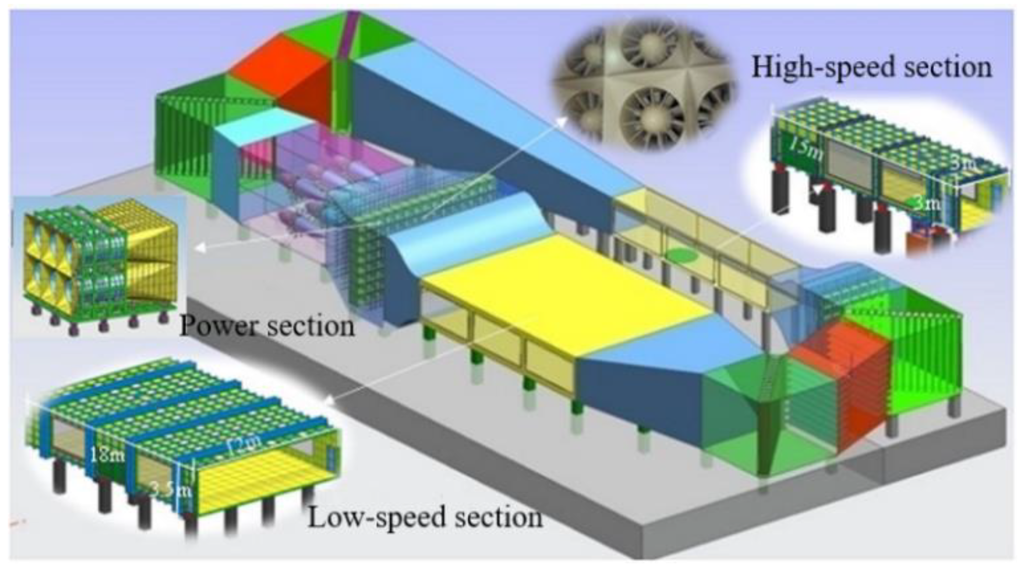
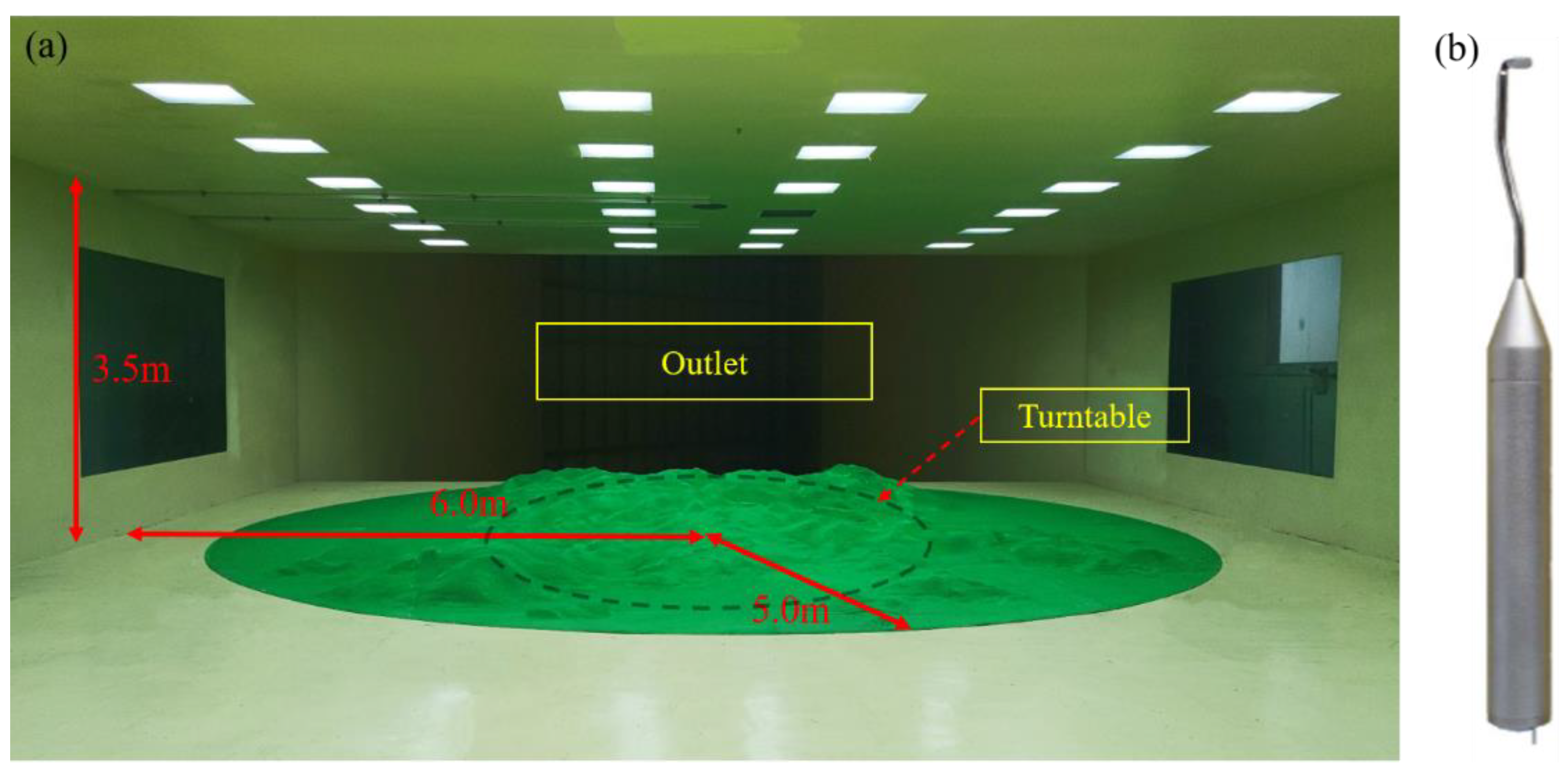
The wind tunnel test was conducted in the low-speed section of the wind tunnel laboratory of Central South University (Figure 4) in Changsha, Hunan Province, which is an important part of the “National Engineering Laboratory for High-speed Railway Construction Technology”, completed in June 2012. The wind tunnel is a large reflux low-speed boundary layer wind tunnel with two test sections in parallel. The power system is composed of six axial flow fans (rated power 335 kw) driven by DC motor, which are divided into 3 (row) × 2 (column) arrangement. The wind tunnel has two test sections. The low-speed test section has a width of 12 m, a height of 3.5 m and a length of 18 m. The wind speed range is 0–20 m/s and the turbulence is less than 1%. The high-speed test section has a width of 3 m, a height of 3 m and a length of 15 m. The maximum wind speed is 0–94 m/s and the turbulence is less than 0.5%.
3.2. Experimental Model
Considering the size of the low-speed wind tunnel, an island terrain model with a geometric scale of 1:1300 is designed and made to simulate the terrain range with a diameter of 13 km. As shown in Figure 5, the terrain model of polyethylene foam 1:1300 ratio is used for stratification and overlap according to contour lines. The diameter of the model is 10 m, the maximum is no more than 0.5 m, and the blocking ratio is about 3.27%, which is lower than the recommended value of 5%.
The value of Reynolds number in this study is in the range of 1.7 × 10⁵–4.6 × 10⁵ studied by Kilpatrick et al. [44]. Their research shows that flow behavior is generally less affected by Reynolds number. For other dimensionless numbers that determine the flow similarity between the wind tunnel test and the real situation, it meets the similarity of Richardson number and Eckert number due to the consideration of the neutral layered boundary layer, and the air working fluid meets the similarity of Prandtl number.
In the test, in order to fully study the characteristics of island wind, wind tunnel tests were carried out in multiple inflows. The measuring instrument is Cobra probe (Figure 5). The high frequency of Cobra probe of turbulence meter is up to 10 kHz, and the measurement accuracy is within ±0.5 m/s. It can be used to measure the velocity at different positions on the terrain model. The test data are sampled at a frequency of 2 kHz. The distance above the ground is measured with a micro laser rangefinder with a measurement accuracy within ±1 mm. On the basis of numerical simulation, five measuring points in three regions are selected, as shown in Figure 2.
4. Numerical Simulation Results
4.1. Determination of Control Wind Direction
In order to deeply explore the wind field of the model by the wind tunnel test, a variety of inflow directions are used in the numerical simulation. Due to the geographical location of the island, the sea breeze often comes from the east of the island. In view of the above characteristics, the simulated working conditions focus on the incoming flow from the east, as shown in Figure 6.
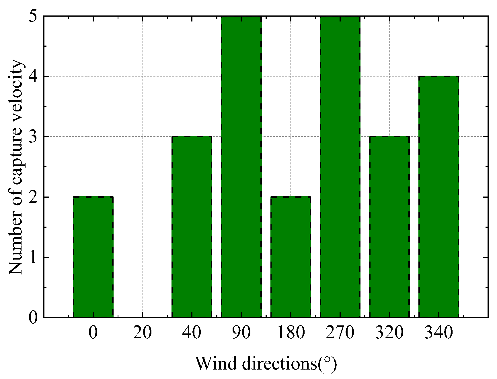
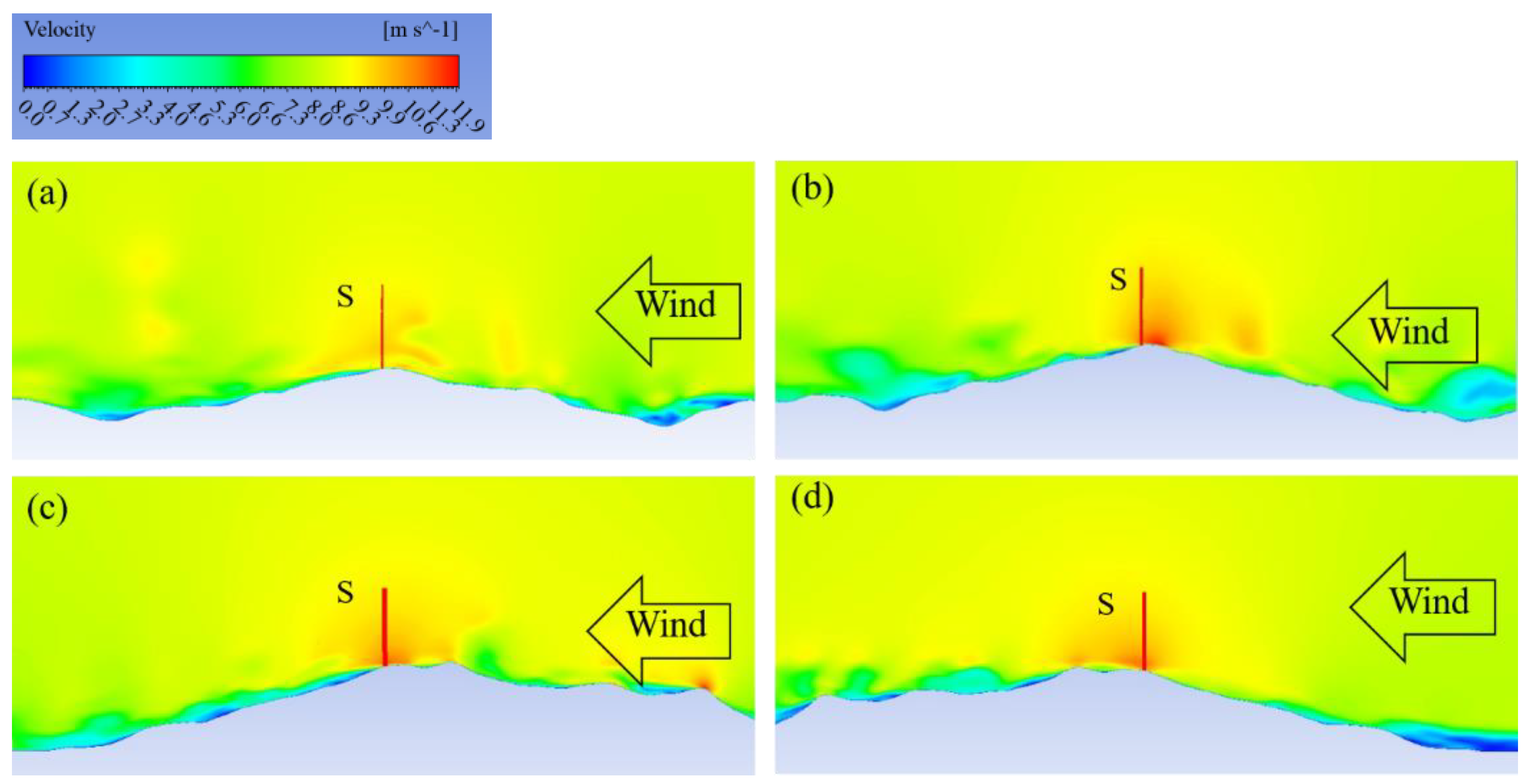
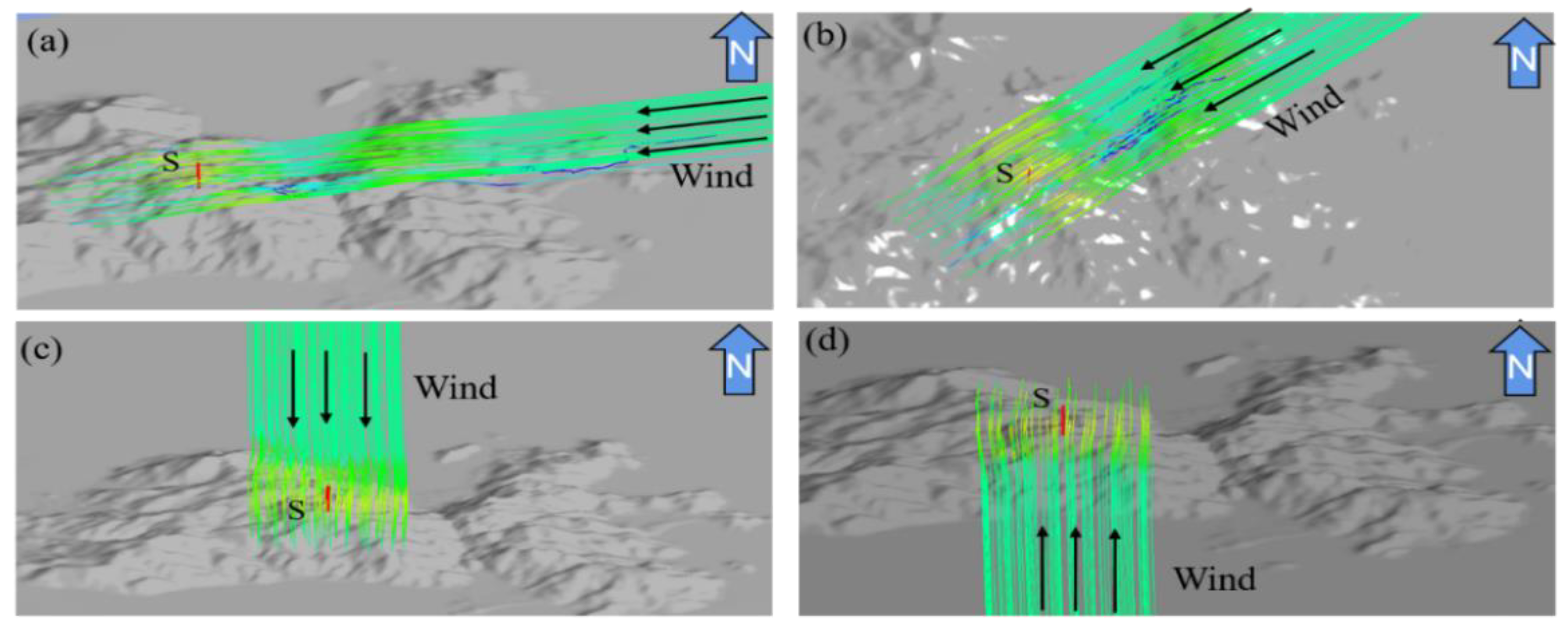
The hub height of most wind turbines is 104 m, so the wind speed at 104 m of each measuring point in the simulation results is statistically analyzed. Specifically, the dimensionless wind speed of each measuring point at a specific height under different wind directions is sorted. The two highest wind speeds are selected as the control wind speed, and the results of each incoming flow are shown in Figure 7. It can be seen from Figure 6 that the number of control wind speeds under 90° and 270° inflow is the largest, while there is no control wind speed at each measuring point under 20° inflow. The wind speed is closely related to the location of the measuring point. The incoming flow entering from different directions will be disturbed by the different terrain. Therefore, the wind speed at the same measuring point under different incoming flows will also change greatly. The most common wind direction of the island is 40°, so this paper selects 40°, 90° and 270° as the control wind direction for further research. The highest point was chosen as an example to illustrate this result. Figure 8 shows the vertical velocity cloud map of a mountain top measuring point (S, Red line) under the inflow of 20°, 40°, 90° and 270°. The normal of each section is perpendicular to the inflow. The streamline diagram of each incoming flow is shown in Figure 9.
As shown in Figure 8, the acceleration effect occurs at vertex s under four wind directions, but the speed of S is different. The velocity of s measuring point is the smallest under 20° inflow, and the acceleration along the height direction is not as obvious as other incoming flows. It can be seen from Figure 8a that the incoming flow will pass through a valley before reaching points, where it turns around with low wind speed, and then continues to advance along the hillside to points. Compared with the 40° inflow in Figure 8b, the acceleration distance of 20° is shorter, so the wind speed is smaller. When the inflow enters the island from 90° and 270°, the forward process is relatively flat and not greatly affected, so the wind speed is large.
From the above analysis, it can be seen that when the incoming flow enters the island from 90° and 270°, the forward process is relatively flat and not greatly affected, so the wind speed is large. The only large valley on the island strikes from north to south, which is consistent with the two incoming flow directions. On the whole, other inflow directions are greatly affected, and even spiral airflow appears. Therefore, from the wind speed analysis, the control wind direction is 90° and 270°. In addition, considering that the most common wind direction in reality is 40°. The incoming flow of subsequent wind tunnel tests adopts the above three wind directions.
4.2. Comparison between Wind Tunnel Test and Numerical Simulation
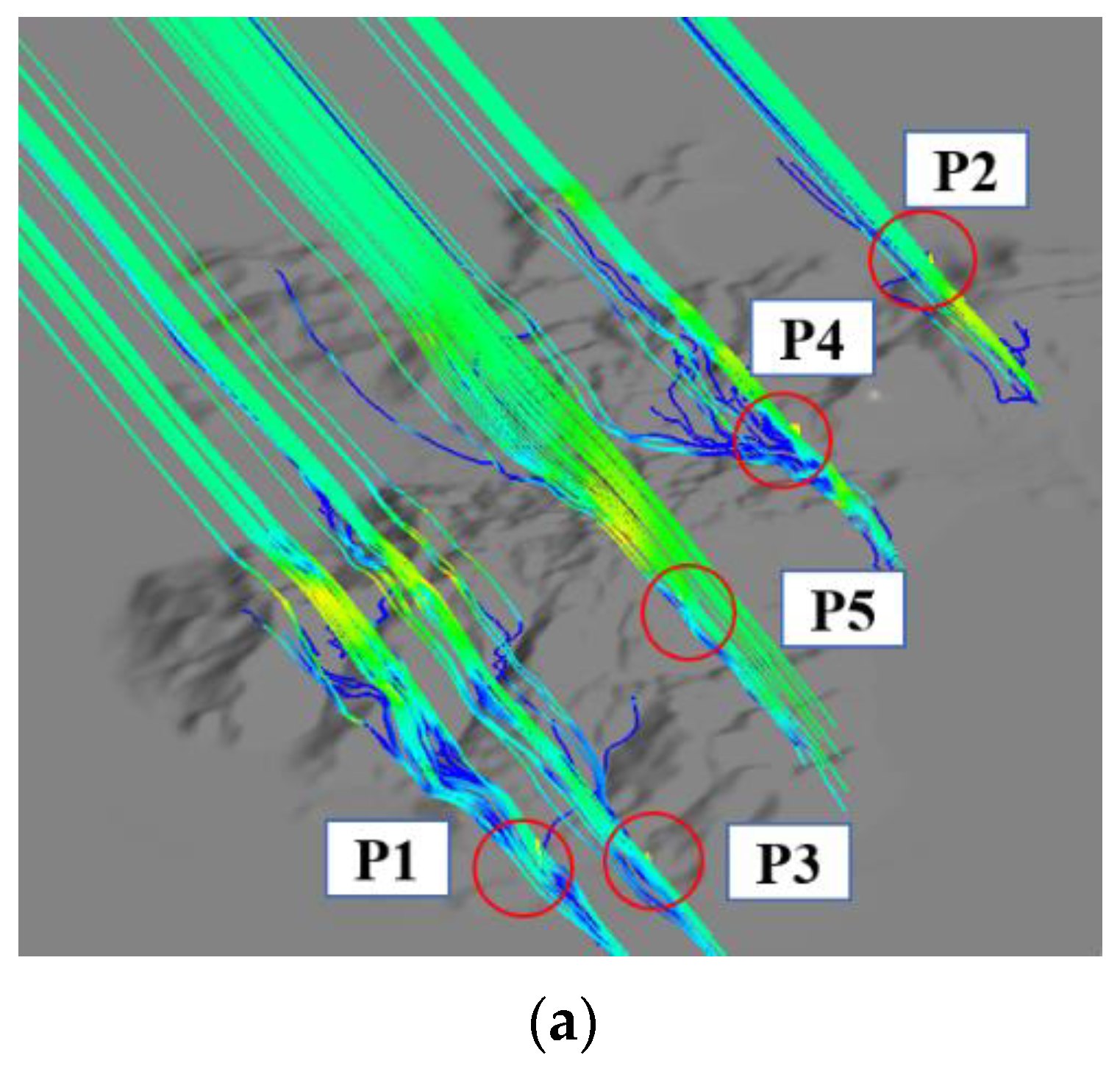
Based on the numerical simulation, the flow conditions in three control directions were carried out in the wind tunnel test, and the wind speeds of five measuring points were monitored. The positions of the measuring points are as shown in Figure 2. These measuring points are distributed in areas with different topographic characteristics on the island. P1 and P3 are located in a relatively flat area of the model, and the distance is relatively close. P2 and P5 are located on the hillside, P4 is located in the internal valley. Among them, the elevation of P5 is the largest and the elevation of measuring point P1 is the smallest.
Figure 10 is the streamline diagram of each measuring point under three control wind directions. It can be seen from the figure that the state of air flow under different inflows is quite different. Compared with 90° and 270°, the air flow fluctuates the most after entering at 40°. At the same time, there are also great differences in the air flow at the measuring points in different areas.
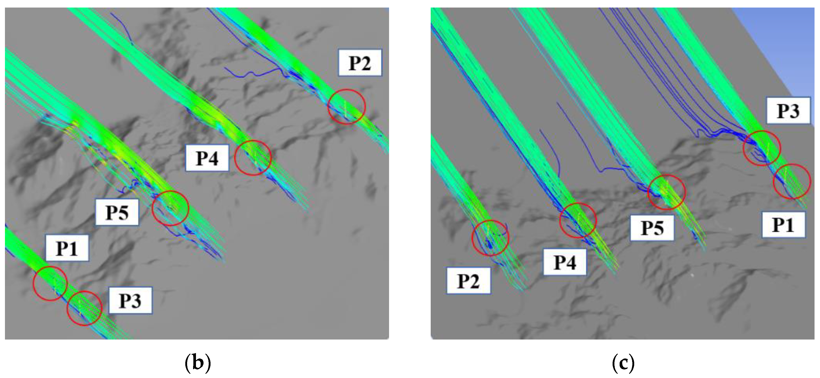
The profile of flow velocity U is normalized by the average velocity Ur of the inflow to reduce the influence of simulation and test errors: U/Ur. Figure 11 shows the velocity results of the numerical simulation and wind tunnel test at the height of 104 m at each measuring point. It can be seen from the figure that the errors of the two results are different, but the values are mainly within 20%. Under this error, it is feasible to use numerical simulation for comprehensive qualitative analysis. The accurate analysis depends on the wind tunnel test, which greatly improves the accuracy of the research [45].
5. Wind Tunnel Test Results
As a result of the above research, the control wind direction of the island was determined, and the accuracy of the numerical simulation was checked. Then, wind characteristics in different regions were studied in depth through wind tunnel tests.
5.1. Mean Velocity
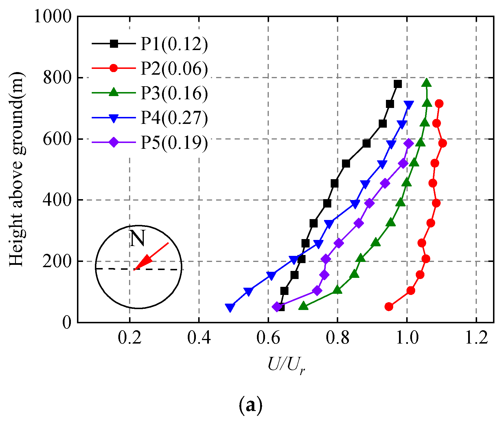
The profile of the flow velocity U is normalized by the average velocity Ur of the inflow. Figure 12 shows the normalized wind speed profile of each measuring point under different inflows and gives the corresponding wind profile coefficients. It can be seen from the figure that the wind profile coefficient shows great discreteness, which is quite different from the recommended value of 0.12 in the specification. It shows that the shape of the wind profile in different areas is different. Among them, the wind profile coefficient of each measuring point under 90 ° inflow is the closest to the standard value. As shown in Figure 12a, the wind speed at P2 under 40° inflow is the largest, which is mainly because there are no mountains or small islands in front of P2. In the process of climbing along the hillside where P2 is located, the wind speed increases and the wind profile develops well. In contrast, other measuring points have low wind speed due to the shielding of mountains of different sizes. Although P5 is situated on the leeward slope, the wind speed is low only at the lowest point of the ground due to the high altitude. For flat areas, the inflow reaches P1 after passing through the whole terrain, so the wind speed at P1 is generally low. The inflow develops well after the recovery over lower terrain before reaching P3, so the wind speed is different from P1. P4 in the valley is located at the lowest part of the downhill of the air flow, where the air flow is greatly disturbed, resulting in a low wind speed below 200 m. But after 200 m, the speed also increases gradually.
As shown in Figure 12b, each measuring point forms a better wind profile under the 90° inflow. The wind speeds of P2 and P3 are the highest, which have a great connection with the clear space ahead of them. The wind profiles of P1, P4 and P5 are relatively close, and the inflow is disturbed before reaching the three measuring points from 90°. It is worth noting that the wind speed of P4 is large at 400 m, but the wind speed changes little after that. This may be due to the acceleration effect of the valley; the wind speed near the ground increases more than that at high altitude.
The wind profile of P3 in Figure 12c is irregular. This is mainly because P3 is in the nearest place to be covered by mountains under the inflow. There is also a barrier in front of P2 but the wind speed is high. The reason is that the change in terrain elevation is relatively stable after crossing the barrier. Moreover, it can be seen that the wind speed of P2 below 200 m also changes greatly, which is affected by blocking. The wind speed of P5 is the largest among all the measuring points. From the terrain analysis, P5 is on the windward slope with large elevation, and the air flow has been fully accelerated. The wind profiles of P1 and P4 are close, and the wind speed is at a medium level.
For the wind speed, the local topographic characteristics and the incoming wind direction play a joint role. The wind speed at the same measuring point varies greatly under different inflows, and the wind speed at different measuring points is also greatly different under the same inflow. This needs to be deeply analyzed in combination with the terrain. Combined with the above analysis, the wind speed on the windward slope is often large. For valleys or relatively flat areas, it is necessary to deeply explore the change in wind speed according to the surrounding terrain.
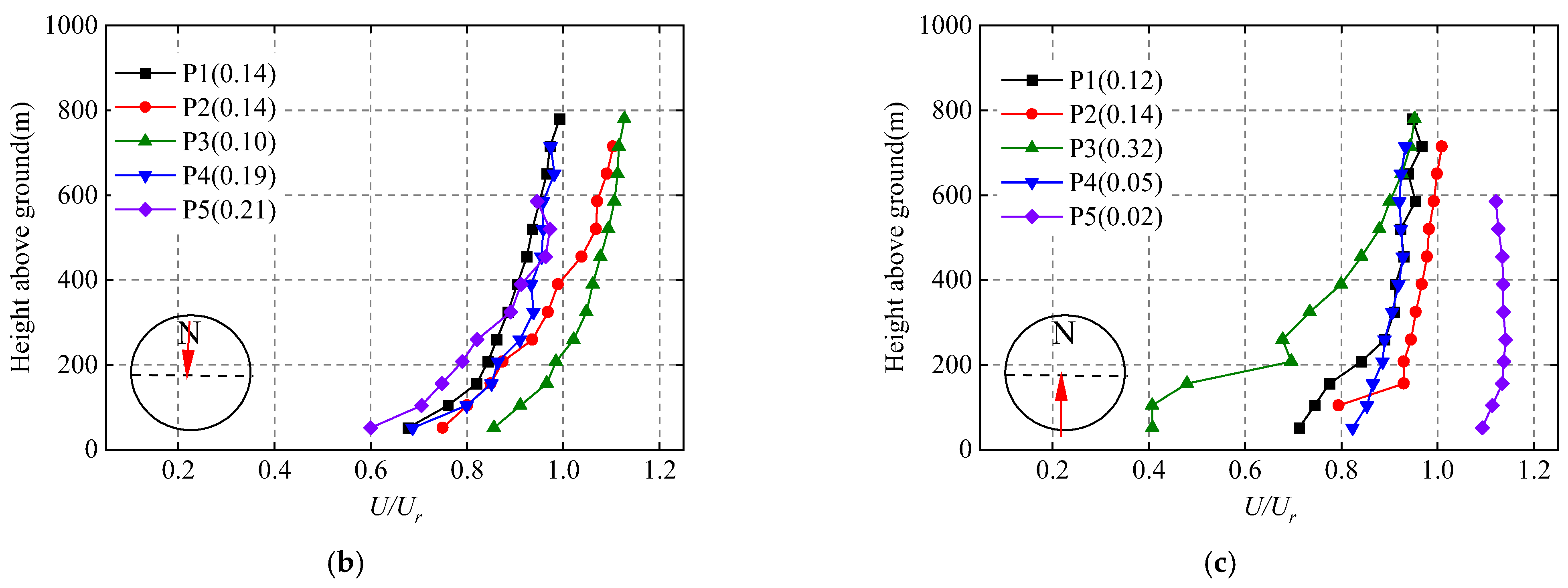
5.2. Wind Attack Angle
The wind attack angle is a wind parameter that describes the degree of airflow fluctuation and represents the magnitude of the vertical wind speed relative to horizontal wind speed. Generally speaking, the value of the wind attack angle on flat terrain is often small, while the wind attack angle often becomes complex due to the irregular change in air flow in hillsides and valleys. Figure 12 shows the variation in the wind attack angle of each measuring point with the height under different inflows. The wind attack angle is mainly in the range of −10°~10°, and the value of the wind attack angle tends to decrease with the increase in height.
As shown in Figure 13a, the values of the wind attack angle at each height of P2 are positive. The reason is because the airflow is climbing at 40° and the direction of the wind speed is upward. Other measuring points (P3, P4 and P5) are located in the leeward area where the air flow often jumps or subducts downward, resulting in negative wind attack angles. The test results at 90° are similar to those at 40°, but there are some differences at the same time. The values of the wind attack angle at P2 are reduced to within 5°, and the wind attack angle of P5 is increased to −10°. The main reason is because compared with 40°, the upward slope at P2 becomes smaller and the downward slope at P5 increases when the inflow enters from 90°. The wind attack angles of other measuring points are also negative. Different from the first two inflows, the wind attack angle of each measuring point changes greatly under the 270° inflow. Due to the conversion of the windward and leeward area where the measuring point is located, the positive and negative wind attack angles change. Most of the wind attack angles of P2 are negative, and the wind attack angles of other measuring points are mainly positive.
Therefore, the positive and negative wind angle of attack is mainly controlled by the incoming wind direction, and the local terrain affects the value of the attack.
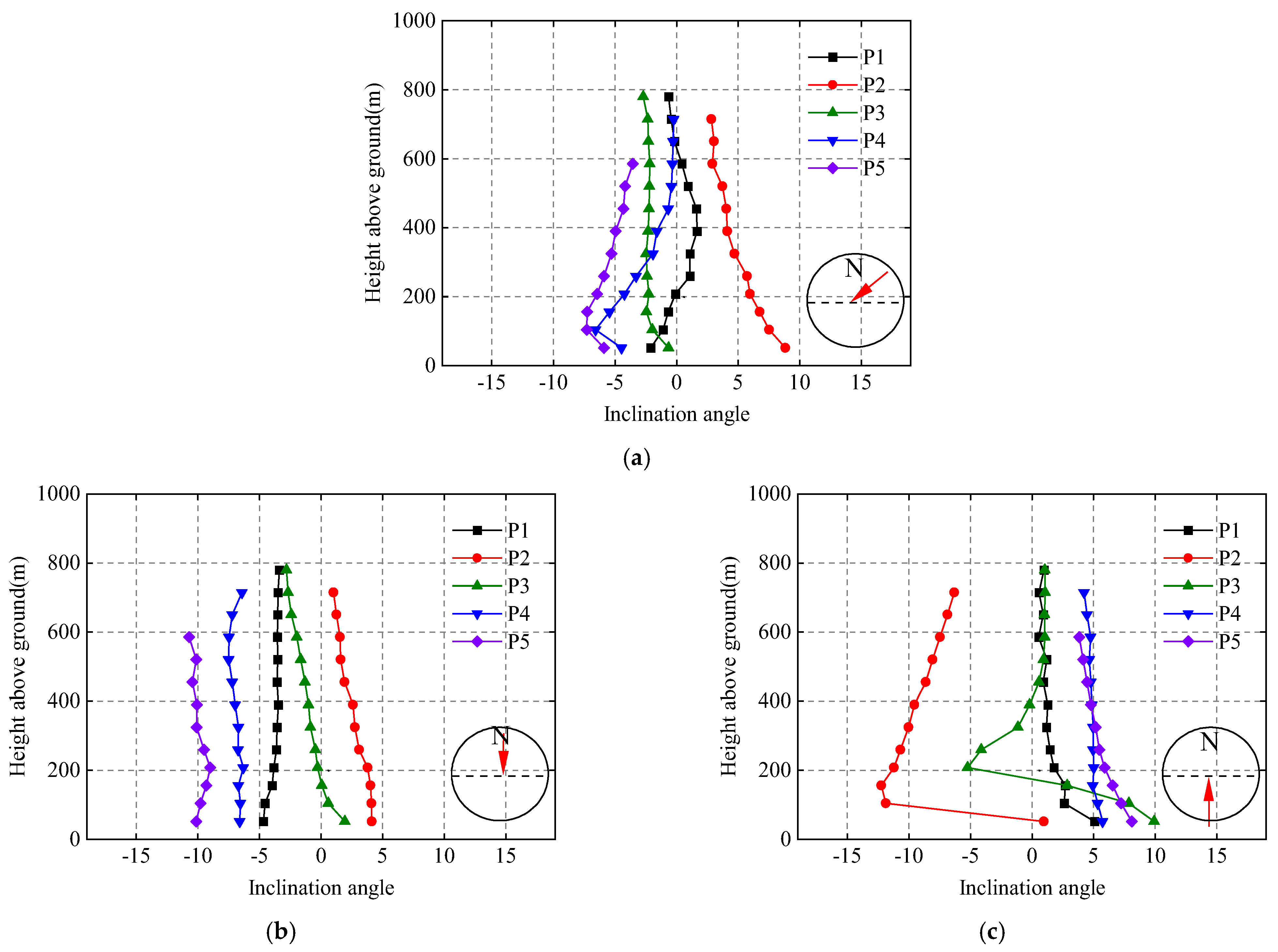
5.3. Turbulence Intensity
Turbulence intensity can quantify the severity of velocity fluctuations. As shown in Figure 14, the turbulence intensity gradually decreases with the increase in height. Compared with the turbulence intensity 0.12 at 10 m height recommended by the specification, the turbulence intensity at most measuring points is large. The turbulence intensity of P2 is the smallest of all measuring points at 40°, while the turbulence intensity of P5 on the hillside is larger. This is related to the windward slope and leeward slope of the two points. The turbulence intensity of P1 and P3 in a flat area is also different due to the different disturbance degree of the incoming flow. In addition, the turbulence intensity of the measurement points presents the stratification phenomenon. Below 200 m, the turbulence intensity is the largest at P4 in the valley; at 200 m or more, the turbulence intensity at P1, where the inflow is last to reach, is the largest.
It can be seen from Figure 14b that the turbulence intensity profiles of each measuring point are relatively close. The turbulence intensity of P2 is high due to the existence of a small mound in front of P2. P5 is located on the leeward slope, so the turbulence intensity near the ground is relatively large. The turbulence intensity of P3 is small because the incoming flow has developed over a certain distance. At the same time, the turbulence intensity of P1 in the flat area is slightly higher. In addition, the turbulence intensity in the valley is at a medium level.
In Figure 14c, the turbulence intensity of P3 in the flat area is larger, which is due to the large fluctuation in wind speed here due to the bulge in front of P3. The turbulence intensity of P1 is smaller than that of P3. It can be observed that the turbulence intensity at the lowest point of P2 reaches 0.4. This may be because there is also a height dividing point for the air separation at the top of the mountain in front of P2. At this height, the air flow is chaotic and the turbulence intensity increases. Above this height, the turbulence intensity of P2 decreases because the air flow separation has ended. The turbulence intensity of P5 is the lowest because it is close to the top of the mountain. Although the air flow is climbing, it has stabilized. Similarly, the turbulence intensity in the valley is at a medium level.
It can be seen from the above test results that the turbulence intensity is controlled by the incoming wind direction and local terrain. If the inflow develops stably, the turbulence intensity is small, and if it is in a disturbed state, the turbulence intensity is large.
5.4. Wind Power Spectra
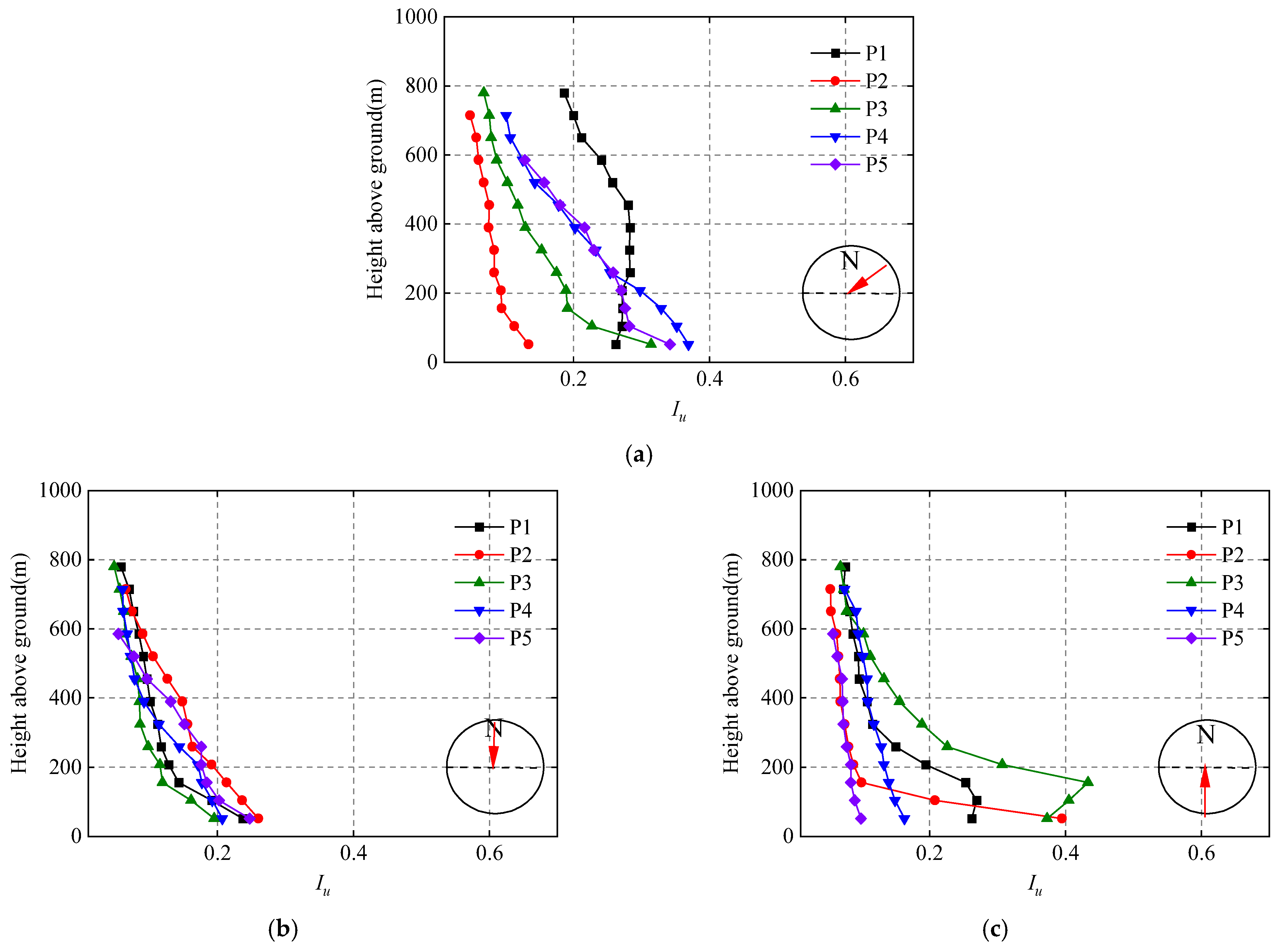
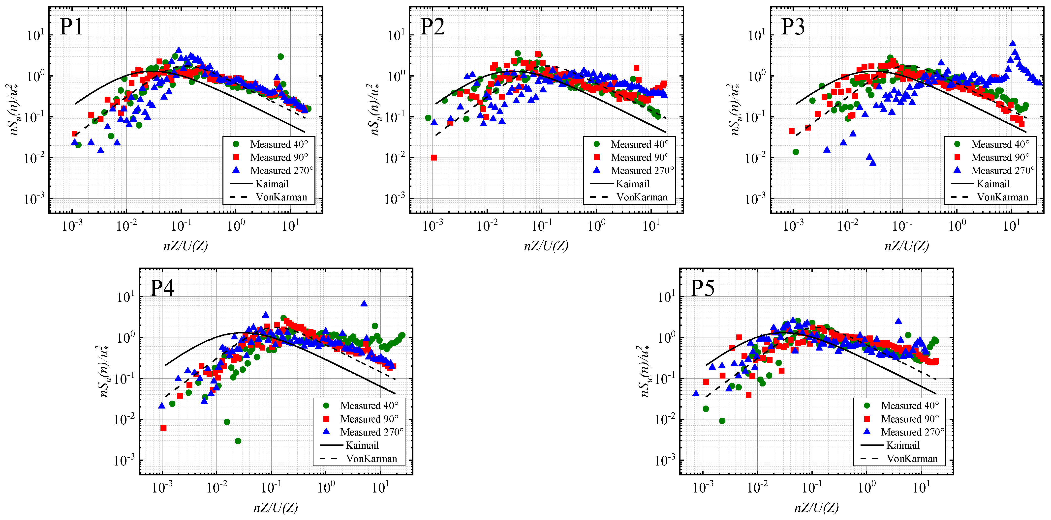
Due to the different undulation degree of different terrains, the energy distribution of fluctuating wind speed power spectra on different terrains may change greatly. Most of the empirical spectra used in the project are based on flat areas, so it is necessary to explore the difference between the empirical spectra and the actual spectra. Two empirical spectra are proposed by Kaimal [46] and von Karman [47]. The comparison between the measured wind spectra and empirical spectra of the measuring points under different inflows is shown in Figure 15. From the results, the fluctuating wind speed power spectra of each measuring point are more consistent with the von Karman spectrum. The Kaimal spectrum overestimates low-frequency energy and underestimates high-frequency energy. Therefore, the von Karman spectrum is more suitable for this terrain. For each measuring point, the measured spectrum is also different under different inflow conditions. This is because the energy value at different frequencies of the wind changes obviously with different terrain, while the energy change of the downflow in flat areas is basically the same no matter which direction it enters from. Therefore, the study of the fluctuating wind speed power spectrum on complex terrain still needs to consider the incoming wind direction.
Compared with other inflows, the low-frequency energy of P1 and P3 in the flat position are lower at 270°, and the high-frequency energy of P3 increases significantly. This is because the front flow of P3 is blocked by the mountain, and the vortex scale of the air flow is significantly reduced, resulting in the increase in high-frequency energy and the decrease in low-frequency energy. The difference is that the 270° inflow will develop smoothly for a period of time before reaching P1, so its high-frequency energy changes little. The power spectra of P2 on the hillside is the same as the above two points, while the situation of P5 and P2 is just the opposite. P4 in the valley is not blocked under the 270° inflow, but is greatly blocked by mountains under the 40° inflow. Therefore, the low-frequency energies of the measured spectra are lower and the high-frequency energies are higher under the 40° inflow.
In order to quantify the movement of the power spectrum energy along the frequency, three standardized frequencies fl, fm and fu are solved, which represent the cutoff frequencies of different energy intervals. This frequency is derived from the following equation
where ln is the natural logarithm. n is the frequency, and nSu(n)/σ2 is nonnegative and integrates to one in (−∞, +∞), and c = l, m, u. The value of ac varies with c, and al = 0.05, am = 0.5 and au = 0.95. Hence, the bandwidth between fl and fu, which means 90% energy interval bandwidth, is calculated from Equation (7)
Figure 16 shows the standardized frequency and 90% energy interval bandwidth of different measuring points under each inflow. As shown in Figure 16a, the median value of the P2 standardization frequency is the smallest, and the median values of the P4 and P5 standardization frequency are the largest. This shows that the power spectra of P4 moves to the higher frequency to the greatest extent, while the power spectra energies of P2 are concentrated in the middle and lower sections. The bandwidths of P2 and P3 are the largest, and the bandwidth of P4 is the smallest. This means that the difference between P2 and P3 is more widely distributed along the standardized frequency and narrower at P4 and P5. The results at 90° inflow are mostly similar to those at 40°, and the median normalized frequencies of P4 and P5 are the largest. The difference is that the median value of the P3 standardized frequency is close to P2 at this time, indicating that the P3 power spectrum energy moves to the low-frequency part again due to the disappearance of the shelter. As shown in Figure 15b, the bandwidth of P2 is largest and P4 is smallest. These results changed at 270°. The median value of the normalized frequency is the smallest at P5 and the largest at P3. It has the largest bandwidth at P2 and P5 and the smallest bandwidth at P1 and P3. To sum up, it can be seen that the bandwidth on the hillside generally maintains a large value, which does not change greatly due to the change in incoming flow direction. In addition, the relevant results of the valley are the opposite. For flat areas, the bandwidth is greatly affected by the direction of the inflow. The change in the median value of the standardized frequency is consistent with the analysis of the above power spectrum. It is larger when it is blocked and smaller when it disappears.
6. Conclusions
By means of numerical simulation and a wind tunnel test, a terrain model of an island within 13 km of 1:1300 is established, and the wind characteristics of the terrain are discussed. Once the control wind directions are determined by numerical simulation, the wind tunnel test is conducted in conjunction with the most common wind direction in practice. A series of studies makes it possible to draw the following conclusions:
(1) The wind profile coefficient is discrete, which is quite different from the recommended value of 0.12. Due to the influence of topography, the wind profile coefficients of different topographic characteristic areas under the same flow are different, and even the wind profile coefficients of the same measuring point under different flows are also different. For the hillside area, the wind speed on the windward slope is larger and the wind speed on the leeward slope is smaller, which is related to the elevation. The wind speed in flat areas is related to the incoming wind direction. When the incoming flow is not blocked, the wind speed is larger, and when blocked, the wind speed decreases. The wind speed in the valley is often low, and as the incoming current enters along the valley, it will have some acceleration effect in the low-level area.
(2) The wind attack angles of each measuring point under different inflows are mainly in the range of −10°~10°. As the height increases, the value of the wind attack angle tends to decrease progressively, but it is much higher than in plain areas. The wind attack angles of the windward slope are positive and those of the leeward slope are negative, both of which are often large. In addition, the wind attack angles in the valley are relatively large, and most of the wind attack angles in flat areas are small. It can be seen that the positive and negative wind attack angles are controlled by the incoming wind direction and the size is closely related to the local terrain.
(3) The turbulence intensity on the windward slope is related to the elevation, which is larger near the foot of the mountain and smaller near the top of the mountain. The turbulence intensity of the leeward slope is larger near the ground. The turbulence intensity in the valley is generally large, and the turbulence intensity in the flat area is controlled by the surrounding terrain. No matter where the measuring point is located, it is different from the specification value of 0.12. In general, it should be significantly greater than 0.12. The fluctuating wind speed power spectrum on the island is more consistent with the von Karman spectrum, which is quite different from the Kaimal spectrum. As the complexity of the local terrain increases, the energy distribution shifts to high frequency. In addition, the bandwidth on the hillside is always at a great value, whereas the valley is the opposite, and the bandwidth of flat areas is greatly affected by the direction of the inflow.
(4) This study shows that the wind characteristics of different areas on the island terrain are quite different, and they are more complex due to the variability in wind direction. The installation position of the turbine needs to consider the combined effects of wind speed, wind attack angle and pulsation characteristics. In addition, it is feasible to study the wind characteristics through the combination of a wind tunnel test and numerical simulation.
Author Contributions
Conceptualization, Y.Z. and Q.L.; methodology, X.H. and Y.Z.; software, P.Y.; validation, Y.Z., P.Y. and X.H.; formal analysis, P.Y.; investigation, Y.Z.; resources, Y.Z.; data curation, P.Y.; writing—original draft preparation, P.Y.; writing—review and editing, Q.L.; visualization, P.Y. and Z.W.; supervision, X.H.; project administration, Q.L.; funding acquisition, Z.W. All authors have read and agreed to the published version of the manuscript.
Funding
This research was funded by the National Natural Science Foundation of China, grant number 52078504, the Science and Technology Innovation Program of Hunan Province (Project No. 2021RC3016), the State Key Laboratory of Mechanical Behavior and System Safety of Traffic Engineering Structures (Project No. KF2021-05), and the Graduated Research Innovation Program of Central South University (Project No.1053320216522).
Institutional Review Board Statement
Not applicable.
Informed Consent Statement
Not applicable.
Data Availability Statement
Data are contained within this article.
Conflicts of Interest
The authors declare no conflict of interest.
Nomenclature
| RANS | Reynolds-Averaged Navier–Stokes |
| LES | Large Eddy Simulation |
| N–S equation | Navier–Stokes equations |
| U | Streamwise velocity |
| Ur | Mean velocity at the top height of each location |
| Iu | Turbulence intensity |
| Su | Streamwise velocity spectra |
| n | Frequency |
| σ | Standard deviation of velocity |
| f | Normalized frequency |
| Z | Height above ground |
| U(Z) | Mean velocity at height Z |
| fl | Cutoff frequency of 0.05 energy interval |
| fm | Cutoff frequency of 0.5 energy interval |
| fu | Cutoff frequency of 0.95 energy interval |
| Δf | 90% energy interval bandwidth |
References
- Arteaga-López, E.; Angeles-Camacho, C. Innovative Virtual Computational Domain Based on Wind Rose Diagrams for Micrositing Small Wind Turbines. Energy 2020, 220, 119701. [Google Scholar] [CrossRef]
- Rokenes, K.; Krogstad, P.A. Wind tunnel simulation of terrain effects on wind farm siting. Wind Energy 2009, 12, 391–410. [Google Scholar] [CrossRef]
- Ishihara, T.; Qi, Y. Numerical Study of Turbulent Flow Fields Over Steep Terrain by Using Modified Delayed Detached-Eddy Simulations. Bound. Lay. Meteorol. 2019, 170, 45–68. [Google Scholar] [CrossRef]
- Porté-Agel, F.; Bastankhah, M.; Shamsoddin, S. Wind-Turbine and Wind-Farm Flows: A Review. Bound. Lay. Meteorol. 2020, 174, 1–59. [Google Scholar] [CrossRef] [Green Version]
- Kozmar, H.; Bartoli, G.; Borri, C. The effect of parked wind turbines on wind flow and turbulence over a complex terrain. Wind Energy 2021, 24, 1337–1347. [Google Scholar] [CrossRef]
- Jackson, P.S.; Hunt, J.C.R. Turbulent Wind Flow Over a Low Hill. Q. J. R. Meteorol. Soc. 1975, 101, 929–955. [Google Scholar] [CrossRef]
- Britter, R.E.; Hunt, J.C.R.; Richards, K.J. Air Flow Over a Two-dimensional Hill: Studies of Velocity Speed-up, Roughness Effects and Turbulence. Q. J. R. Meteorol. Soc. 1981, 107, 91–110. [Google Scholar] [CrossRef]
- Nanni, S.C.; Tampieri, F. A Linear Investigation on Separation in Laminar and Turbulent Boundary Layers Over Low Hills and Valleys. Nuovo Cim. C 1985, 8, 579–601. [Google Scholar] [CrossRef]
- Wood, N. The Onset of Separation in Neutral, Turbulent Flow Over Hills. Bound. Lay. Meteorol. 1995, 76, 137–164. [Google Scholar] [CrossRef]
- Walmsley, J.L.; Taylor, P.A.; Keith, T. A simple model of neutrally stratified boundary-layer flow over complex terrain with surface roughness modulations (MS3DJH/3R). Bound. Lay. Meteorol. 1986, 36, 157–186. [Google Scholar] [CrossRef]
- Taylor, P.A.; Walmsley, J.L.; Salmon, J.R. A simple model of neutrally stratified boundary-layer flow over real terrain incorporating wavenumber-dependent scaling. Bound. Lay. Meteorol. 1983, 26, 169–189. [Google Scholar] [CrossRef]
- Hu, W.; Yang, Q.; Chen, H. Wind field characteristics over hilly and complex terrain in turbulent boundary layers. Energy 2021, 224, 120070. [Google Scholar] [CrossRef]
- Ying, R.; Canuto, V.M. Numerical Simulation of Flow Over Two-dimensional Hills Using a Second-order Turbulence Closure Model. Bound. Lay. Meteorol. 1997, 85, 447–474. [Google Scholar] [CrossRef]
- Kim, H.G.; Lee, C.M.; Lim, H.C. An Experimental and Numerical Study on the Flow Over Two-dimensional Hills. J. Wind Eng. Ind. Aerodyn. 1997, 66, 17–33. [Google Scholar] [CrossRef]
- Lun, Y.; Mochida, A.; Murakami, S. Numerical Simulation of Flow Over Topographic Features By Revised K-ϵ Models. J. Wind Eng. Ind. Aerodyn. 2003, 91, 231–245. [Google Scholar] [CrossRef]
- Abdi, D.S.; Bitsuamlak, G.T. Wind Flow Simulations on Idealized and Real Complex Terrain Using Various Turbulence Models. Adv. Eng. Softw. 2014, 75, 30–41. [Google Scholar] [CrossRef]
- Ross, A.N.; Arnold, S.; Vosper, S.B. A Comparison of Wind-tunnel Experiments and Numerical Simulations of Neutral and Stratified Flow Over a Hill. Bound. Lay. Meteorol. 2004, 113, 427–459. [Google Scholar] [CrossRef]
- Iizuka, S.; Kondo, H. Large-eddy Simulations of Turbulent Flow Over Complex Terrain Using Modified Static Eddy Viscosity Models. Atmos. Environ. 2006, 40, 925–935. [Google Scholar] [CrossRef]
- Wan, F.; Porte-Agel, F.; Stoll, R. Evaluation of Dynamic Subgrid-scale Models in Large-eddy Simulations of Neutral Turbulent Flow Over a Two-dimensional Sinusoidal Hill. Atmos. Environ. 2007, 41, 2719–2728. [Google Scholar] [CrossRef]
- Cao, S.; Tong, W.; Ge, Y. Numerical Study on Turbulent Boundary Layers Over Two-dimensional Hills—Effects of Surface Roughness and Slope. J. Wind Eng. Ind. Aerodyn. 2012, 104–106, 342–349. [Google Scholar] [CrossRef]
- Tamura, T.; Okuno, A.; Sugio, Y. Les Analysis of Turbulent Boundary Layer Over 3d Steep Hill Covered with Vegetation. J. Wind Eng. Ind. Aerodyn. 2007, 95, 1463–1475. [Google Scholar] [CrossRef]
- Liu, Z.; Ishihara, T.; Tanaka, T. Les Study of Turbulent Flow Fields Over a Smooth 3-d Hill and a Smooth 2-d Ridge. J. Wind Eng. Ind. Aerodyn. 2016, 153, 1–12. [Google Scholar] [CrossRef]
- Liu, Z.; Hu, Y.; Yan, Y. Turbulent Flow Fields Over a 3d Hill Covered By Vegetation Canopy Through Large Eddy Simulations. Energies 2019, 12, 3624. [Google Scholar] [CrossRef] [Green Version]
- Bowen, A.J.; Lindley, D. A Wind-tunnel Investigation of the Wind Speed and Turbulence Characteristics Close to the Ground Over Various Escarpment Shapes. Bound. Lay. Meteorol. 1977, 12, 259–271. [Google Scholar] [CrossRef]
- Pearse, J.R.; Lindley, D.; Stevenson, D.C. Wind Flow Over Ridges in Simulated Atmospheric Boundary Layers. Bound. Lay. Meteorol. 1981, 21, 77–92. [Google Scholar] [CrossRef]
- Cao, S.; Tamura, T. Experimental study on roughness effects on turbulent boundary layer flow over a two-dimensional steep hill. J. Wind Eng. Ind. Aerodyn. 2006, 94, 1–19. [Google Scholar] [CrossRef]
- Cao, S.; Tamura, T. Effects of roughness blocks on atmospheric boundary layer flow over a two-dimensional low hill with/without sudden roughness change. J. Wind Eng. Ind. Aerodyn. 2007, 95, 679–695. [Google Scholar] [CrossRef]
- Weerasuriya, A.U.; Hu, Z.; Li, S. Wind Direction Field Under the Influence of Topography, Part I: A Descriptive Model. Wind Struct. 2016, 22, 455–476. [Google Scholar] [CrossRef]
- Weerasuriya, A.U.; Tse, K.T.; Zhang, X. A wind tunnel study of effects of twisted wind flows on the pedestrian-level wind field in an urban environment. Build. Environ. 2018, 128, 225–235. [Google Scholar] [CrossRef]
- Tse, K.T.; Weerasuriya, A.U.; Hu, G. Integrating Topography-modified Wind Flows Into Structural and Environmental Wind Engineering Applications. J. Wind Eng. Ind. Aerodyn. 2020, 204, 104270. [Google Scholar] [CrossRef]
- Weerasuriya, A.U.; Tse, K.T.; Zhang, X. Equivalent Wind Incidence Angle Method: A New Technique to Integrate the Effects of Twisted Wind Flows to Ava. Build. Environ. 2018, 139, 46–57. [Google Scholar] [CrossRef]
- Carpenter, P.; Locke, N. Investigation of Wind Speeds Over Multiple Two-dimensional Hills. J. Wind Eng. Ind. Aerodyn. 1999, 83, 109–120. [Google Scholar] [CrossRef]
- Miller, C.A.; Davenport, A.G. Guidelines for the Calculation of Wind Speed-ups in Complex Terrain. J. Wind Eng. Ind. Aerodyn. 1998, 74–76, 189–197. [Google Scholar] [CrossRef]
- Uchida, T.; Ohya, Y. Micro-siting Technique for Wind Turbine Generators By Using Large-eddy Simulation. J. Wind Eng. Ind. Aerodyn. 2008, 96, 2121–2138. [Google Scholar] [CrossRef]
- Uchida, T.; Ohya, Y. Large-eddy Simulation of Turbulent Airflow Over Complex Terrain. J. Wind Eng. Ind. Aerodyn. 2003, 91, 219–229. [Google Scholar] [CrossRef]
- Blocken, B. CFD simulation of wind flow over natural complex terrain: Case study with validation by field measurements for Ria de Ferrol, Galicia, Spain. J. Wind Eng. Ind. Aerodyn. 2015, 147, 43–57. [Google Scholar] [CrossRef]
- Mcauliffe, B.R.; Larose, G.L. Reynolds-number and Surface-modeling Sensitivities for Experimental Simulation of Flow Over Complex Topography. J. Wind Eng. Ind. Aerodyn. 2012, 104, 603–613. [Google Scholar] [CrossRef]
- Lang, J.; Mann, J.; Berg, J. For wind turbines in complex terrain, the devil is in the detail. Environ. Res. Lett. 2017, 12, 094020. [Google Scholar] [CrossRef]
- Jubayer, C.M.; Hangan, H. A Hybrid Approach for Evaluating Wind Flow Over a Complex Terrain. J. Wind Eng. Ind. Aerodyn. 2018, 175, 65–76. [Google Scholar] [CrossRef]
- Maurizi, A.; Palma, J.; Castro, F.A. Numerical Simulation of the Atmospheric Flow in a Mountainous Region of the North of Portugal. J. Wind Eng. Ind. Aerodyn. 1998, 74–76, 219–228. [Google Scholar] [CrossRef]
- Hu, P.; Li, Y.; Huang, G. The Appropriate Shape of the Boundary Transition Section for a Mountain-gorge Terrain Model in a Wind Tunnel Test. Wind Struct. 2015, 20, 15–36. [Google Scholar] [CrossRef]
- Hu, P.; Han, Y.; Xu, G. Numerical Simulation of Wind Fields at the Bridge Site in Mountain-gorge Terrain Considering an Updated Curved Boundary Transition Section. J. Aerosp. Eng. 2018, 31, 04018008. [Google Scholar] [CrossRef]
- Cuerva-Tejero, A.; Avila-Sanchez, S.; Gallego-Castillo, C. Measurement of spectra over the Bolund hill in wind tunnel. Wind Energy 2018, 21, 87–99. [Google Scholar] [CrossRef]
- Kilpatrick, R.J.; Hangan, H.; Siddiqui, K.; Lange, J.; Mann, J. Turbulent Flow Characterization Near the Edge of a Steep Escarpment. J. Wind Eng. Ind. Aerodyn. 2021, 212, 104605. [Google Scholar] [CrossRef]
- Chen, X.; Liu, Z.; Wang, X. Experimental and Numerical Investigation of Wind Characteristics over Mountainous Valley Bridge Site Considering Improved Boundary Transition Sections. Appl. Sci. 2020, 10, 751. [Google Scholar] [CrossRef] [Green Version]
- Kaimal, J.C.; Wyngaard, J.C.; Izumi, Y.; Coté, O.R. Spectral characteristics of surface-layer turbulence. Q. J. R. Meteorol. Soc. 1972, 98, 563–589. [Google Scholar] [CrossRef]
- Karman, T.V. Progress in the statistical theory of turbulence. Proc. Natl. Acad. Sci. USA 1948, 34, 530–539. [Google Scholar] [CrossRef] [Green Version]
Figure 1.
Satellite topographic map of the island.

Figure 2.
Computational domain with boundary conditions and schematic diagram of measuring points.

Figure 3.
(a) Mesh of the terrain model; (b) local mesh.

Figure 4.
Schematic diagram of the wind tunnel.

Figure 5.
(a) The island terrain model in wind tunnel; (b) the Cobra probe.

Figure 6.
Different inflow conditions of numerical simulation.

Figure 7.
Quantity of capture wind speed under each incoming flow.

Figure 8.
Velocity nephogram (a) 20° (b) 40° (c) 90° (d) 270°.

Figure 9.
Streamline diagram (a) 20° (b) 40° (c) 90° (d) 270°.

Figure 10.
Streamline diagram at measurement locations. (a) 40° (b) 90° (c) 270°.


Figure 11.
Velocity results of numerical simulation and wind tunnel test. (a) 40° (b) 90° (c) 270°.

Figure 12.
Profiles of mean velocity at measurement locations. (a) 40° (b) 90° (c) 270°.


Figure 13.
Profiles of wind attack angle at measurement locations. (a) 40° (b) 90° (c) 270°.

Figure 14.
Profiles of turbulence intensity at measurement locations. (a) 40° (b) 90° (c) 270°.

Figure 15.
Normalized wind speed spectra for measurement locations at the height of 104 m.

Figure 16.
Metrics on spectra shifts at measurement locations. (a) 40° (b) 90° (c) 270°.

Publisher’s Note: MDPI stays neutral with regard to jurisdictional claims in published maps and institutional affiliations. |
© 2022 by the authors. Licensee MDPI, Basel, Switzerland. This article is an open access article distributed under the terms and conditions of the Creative Commons Attribution (CC BY) license (https://creativecommons.org/licenses/by/4.0/).
Share and Cite
MDPI and ACS Style
Zou, Y.; Yue, P.; Liu, Q.; He, X.; Wang, Z. Wind Field Characteristics of Complex Terrain Based on Experimental and Numerical Investigation. Appl. Sci. 2022, 12, 5124. https://0-doi-org.brum.beds.ac.uk/10.3390/app12105124
AMA Style
Zou Y, Yue P, Liu Q, He X, Wang Z. Wind Field Characteristics of Complex Terrain Based on Experimental and Numerical Investigation. Applied Sciences. 2022; 12(10):5124. https://0-doi-org.brum.beds.ac.uk/10.3390/app12105124
Chicago/Turabian StyleZou, Yunfeng, Peng Yue, Qingkuan Liu, Xuhui He, and Zhen Wang. 2022. "Wind Field Characteristics of Complex Terrain Based on Experimental and Numerical Investigation" Applied Sciences 12, no. 10: 5124. https://0-doi-org.brum.beds.ac.uk/10.3390/app12105124
Note that from the first issue of 2016, this journal uses article numbers instead of page numbers. See further details here.