Numerical Computation of Sloshing-Induced Force in Complex Ship Tanks under the Excitation of Ship Rolling Motion Based on the MPS Method

Abstract

Liquid sloshing in ship tanks would have a direct effect on ship dynamic stability, and thus is of great importance for navigation safety. To calculate the sloshing-induced force on real ship tanks, this paper presents an approach to numerically simulate the liquid-sloshing in complex tanks using the moving particle semi-implicit (MPS) method. The sloshing-induced force is numerically calculated and used to investigate the effect of different excitation conditions in which the realistic ship motions under different loading conditions have been taken into account. Simulation results show that the maximum sloshing-induced force is much bigger than the corresponding static one. Meanwhile, both the rolling angle and period have significant effects on liquid sloshing.

1. Introduction

Under the external excitation of the ship’s motion, the phenomena of liquid sloshing will inevitably take place in partially filled liquid tanks of moving ships. In these cases, the traditional quasi-static method assuming the free surface is parallel to the sea level is not suitable for estimating the effect of free surface on ship stability. The sloshing-induced force would have a direct effect on ship dynamic stability [1,2]. Therefore, it is of great importance to determine the sloshing-induced force for navigation safety.

In recent decades, many researchers shifted their attention to the computational fluid dynamics (CFD) technique to solve the liquid sloshing problem, though the computing time may be intimidating [3]. In early years, due to the limitation of computing ability, mesh based numerical methods were mostly employed to investigate the liquid sloshing issues, such as the finite differential method (FDM) [4,5,6,7,8], the finite element method (FEM) [9,10,11,12], the finite volume method (FVM) [13,14,15], the volume of fluid method (VOF) [16,17], and the level-set method (L-S) [18].

Resulting from the use of mesh, however, the mesh based numerical methods suffer from difficulties in dealing with the nonlinear free surface flows. Recently, with the improvement of computing ability, meshfree methods have been widely used to simulate the violent free surface flow with large deformation and nonlinear fragmentation [19]. The key idea of the meshfree methods is to provide accurate and stable numerical solutions for integral equations or partial differential equations (PDEs) with all kinds of possible boundary conditions using a set of arbitrarily distributed nodes or particles [20]. In this way, the meshfree methods overcome the inherent difficulty of the mesh methods, i.e., the mesh distortion caused by large deformation.

A smoothed particle hydrodynamics (SPH) method is one of the popular meshfree methods. SPH was firstly introduced in 1977 [21,22]. The SPH method was firstly applied to address the free surface flow problem in 1994 [23]. After that, SPH methods including weakly-compressible SPH (WCSPH) and incompressible SPH (ISPH) were used to simulate the phenomena of liquid sloshing in partially filled tanks [24,25,26,27,28,29,30,31,32,33,34]. However, the kernel in the SPH method is considered as a mass distribution of each particle. The superposition of the kernels represents the physical superposition of mass. Thus, the particle is like a spherical cloud [35]. This concept may be more fitted to compressible fluids.

Another popular meshfree method is the moving particle semi-implicit (MPS) method. The original MPS method was proposed by Koshizuka and Oka [36] to simulate the incompressible flow. In the original MPS method, there were several defects including non-optimal source term, gradient and collision models, and search of free-surface particles, which led to less accurate fluid motions and non-physical pressure fluctuations [37]. To overcome these defects, many researchers have put forward a series of improvements on the MPS method, including the improvement of the kernel function [38,39], the Laplacian model [40], the collision model [41], the pressure Poisson equation (PPE) [37,42,43,44,45], the pressure gradient model [46,47], and the boundary condition [48,49]. The MPS method has also been widely used to solve the problem of liquid sloshing [50,51,52,53,54,55].

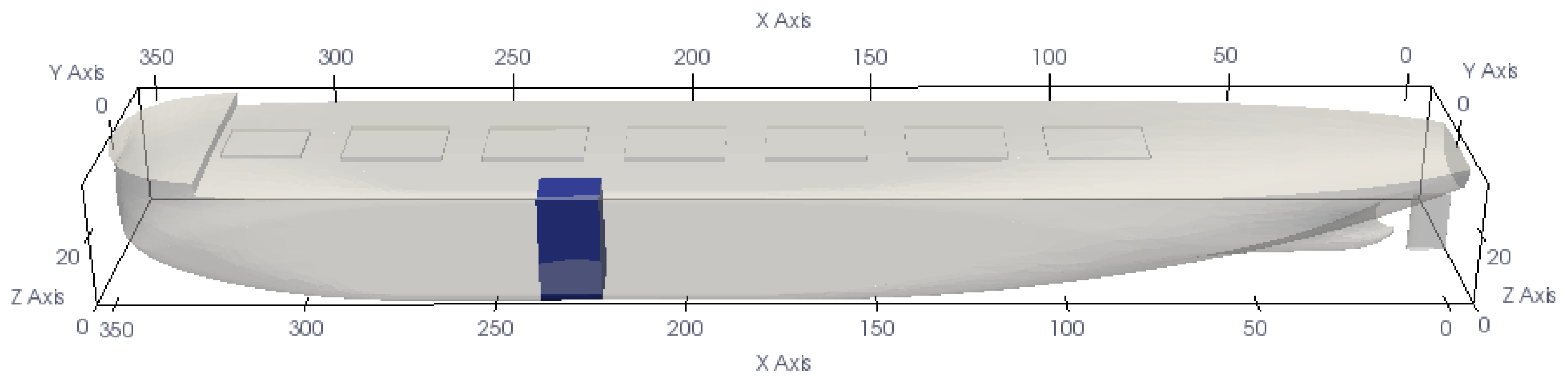
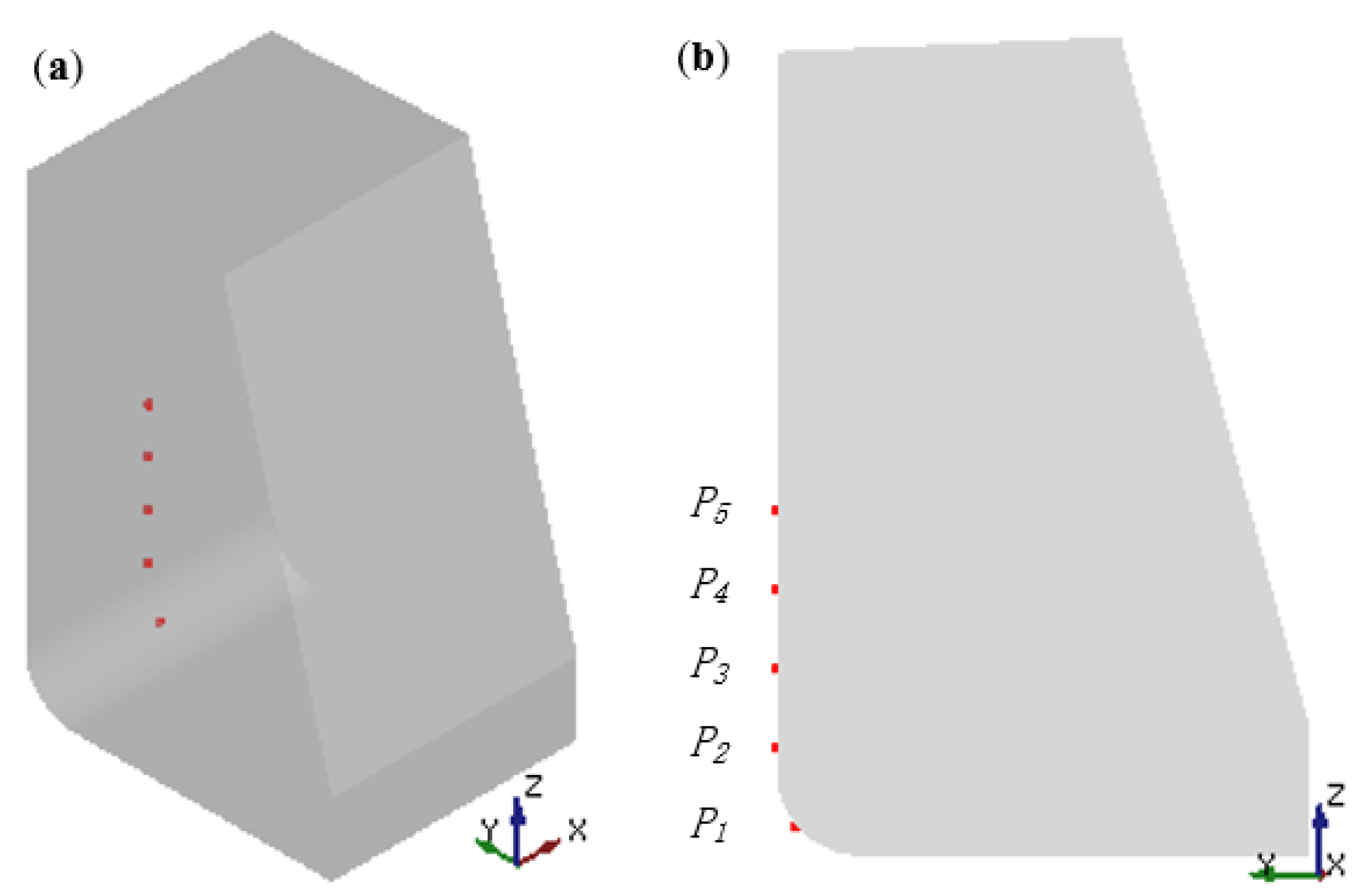
Liquid sloshing in ship tanks has a significant effect on ship dynamic stability. However, the main weaknesses of the current research on liquid sloshing are that most researchers used simplified ship tanks instead of the real ship tanks to simulate liquid sloshing, and do not consider the effect of real ship motion under actual loading conditions. For complicated surface shapes, like structure of arc and slope, equally spaced particle distribution with nearly constant thickness is not readily found [35]. Thus, the initialization of boundary particles in complex tanks is more cumbersome than that in simplified tanks. Furthermore, the solid boundary shape is represented by a finite number of particles, and the representation of the complete details of the geometric information will be more complicated. Although sloshing simulations in real ships are complex, it is necessary for a realistic investigation of sloshing-inducing force. Meanwhile, the excitation period adopted in previous works came from the natural frequencies of gravity waves in an upright resting cylindrical tank [56]. However, this period is different from the rolling period of real ships in most cases. Therefore, the sloshing-induced force in ship tanks under more realistic conditions needs to be further investigated.

This paper aims to compute the dynamic force acting on the bulkhead caused by more realistic excitation in real ship tanks. The efficiency of MPS is generally better than that of WCSPH, but similar to ISPH [57]. From the discrepancies of the kernel function between SPH and MPS methods, the MPS method is more suitable for simulating incompressible fluids than the SPH method. Thus, this paper uses the MPS method to calculate the sloshing-induced force in ship tanks. First, the MPS method used in this paper is verified via numerical simulations of liquid sloshing in a rectangular tank. After that, numerical simulations of liquid sloshing in a real ship tank are carried out. Finally, the sloshing-induced force is computed and analyzed.

The rest of this paper is organized as follows: Section 2 introduces the basic theories of the MPS method. Section 3 verifies the MPS method used in this paper via liquid sloshing simulations. Section 4 gives the numerical results of the liquid sloshing in a real ship tank under different ship rolling motions. Section 5 draws conclusions.

2. MPS Method

The MPS method is based on a fully Lagrangian description. It uses a semi-implicit algorithm to simulate the incompressible viscous flows. In MPS, derivatives in the governing equations are transformed to interactions among the neighboring particles [58]. The MPS method used in this paper is presented as follows.

2.1. Mathematical Formulation

2.1.1. Governing Equations

For an incompressible fluid flow, the governing equations which contain a continuity equation and Navier–Stokes (N–S) equation can be written as follows:

$$\nabla ·\mathit{u}=0$$

(1)

$$\frac{D\mathit{u}}{Dt}=-\frac{1}{\rho }\nabla P+\nu {\nabla }^2\mathit{u}+\mathbf{g}$$

(2)

where $\mathit{u}$, P, $\rho$, $\nu$, t, and $\mathbf{g}$ denote velocity vector of the particle, pressure, fluid density, kinematic viscosity, time, and gravity vector, respectively.

2.1.2. Particle Interaction Model

In the MPS method, functions are approximated by a weighted average approach. In order to avoid non-physical pressure oscillation in an original kernel function, a modified kernel function which was proposed by [50] is employed in this paper, that is:

$$W\left(r\right)=\left\{\begin{array}{cc}\frac{r_e}{0.85r+0.15r_e}-1\hfill & 0\le r<r_e\hfill \\ 0\hfill & r_e\le r\hfill \end{array}\right.$$

(3)

where $r_e$ is the radius of particle interaction, and r is the distance between two particles.

Summation of the weight function is called particle number density, which is used to keep the incompressibility of fluid:

$${\langle n\rangle }_i=\sum _{j\ne i}W\left(|{\mathbf{r}}_j-{\mathbf{r}}_i|\right)$$

(4)

The gradient model is the weighted average of a physical quantity $\varphi$ between particle i and its neighboring particles. It is mainly used to discretize the term of pressure gradient. The model proposed by [35] is adopted here, that is:

$${\langle \nabla \varphi \rangle }_i=\frac{d}{n^0}\sum _{j\ne i}\frac{{\varphi }_j-\widehat{{\varphi }_i}}{{|{\mathit{r}}_j-{\mathit{r}}_i|}^2}({\mathit{r}}_j-{\mathit{r}}_i)W\left(|{\mathit{r}}_j-{\mathit{r}}_i|\right)$$

(5)

$$\widehat{{\varphi }_i}=min({\varphi }_j,{\varphi }_i),\{j:W\left(|{\mathit{r}}_j-{\mathit{r}}_i|\right)\ne 0\}$$

(6)

where d is number of dimension, $n^0$ is initial particle number density, and $\mathit{r}$ is position vector.

The divergence model is used to discrete the velocity divergence in PPE and is similar to the gradient model. It is described as follows:

$${\langle \nabla ·\mathit{u}\rangle }_i=\frac{d}{n^0}\sum _{j\ne i}\frac{({\mathit{r}}_j-{\mathit{r}}_i)·({\mathit{u}}_j-{\mathit{u}}_i)}{{|{\mathit{r}}_j-{\mathit{r}}_i|}^2}W\left(|{\mathit{r}}_j-{\mathit{r}}_i|\right)$$

(7)

The Laplacian model is the weighted average of the distribution of a physical quantity $\varphi$ from particle i to its neighboring particles. This model is used to discretize the viscosity term of PPE and is described as follows:

$${\langle {\nabla }^2\varphi \rangle }_i=\frac{2d}{n^0\lambda }\sum _{j\ne i}({\varphi }_j-{\varphi }_i)W\left(|{\mathit{r}}_j-{\mathit{r}}_i|\right)$$

(8)

where $\lambda$ is a parameter which is used to compensate for a finite range of kernel function, and can be obtained by:

$$\lambda =\frac{\sum _{j\ne i}{|{\mathit{r}}_j-{\mathit{r}}_i|}^{2}W\left(|{\mathit{r}}_j-{\mathit{r}}_i|\right)}{\sum _{j\ne i}W\left(|{\mathit{r}}_j-{\mathit{r}}_i|\right)}$$

(9)

2.1.3. Pressure Poisson Equation

In the MPS method, the pressure is calculated by solving the PPE, which is proposed by [37] as follows:

$${\langle {\nabla }^2{P}^{k+1}\rangle }_i=(\gamma -1)\frac{\rho }{\Delta t}\nabla ·{\mathit{u}}_i^{\ast }-\gamma \frac{\rho }{\Delta t^2}\frac{{\langle n^{\ast }\rangle }_i-n^0}{n^0}$$

(10)

where $\gamma$ is a blending parameter whose range is between 0.01 to 0.05, $n^{\ast }$ is temporal particle density, and $\Delta t$ is time step.

The left-hand side of Equation (10) can be discretized by applying the Laplacian model, as shown in Equation (8). The right-hand side of Equation (10) is the mixed source term, which is given by the divergence-free condition and the deviation of the temporal particle number density from the constant. The term given by the divergence-free condition can be discretized by applying the divergence model, as shown in Equation (7).

2.1.4. Boundary Condition

The MPS method needs to decide on boundary conditions for solving the pressure Poisson equation. The free surface boundary and solid boundary conditions used in this paper are described as follows:

• Free surface boundary. Since no particle can exist outside the fluid domain, the particle number density will inevitably decrease on the free surfaces. Therefore, the particles nearing the free surface can be detected by the following condition:

  $${\langle n\rangle }_i^{\ast }<\beta n^0$$

  (11)

  where $\beta$ is a parameter, and is less than $1.0$.
  Furthermore, the pressure of free surface particles is set to zero.
• Solid boundary. For the moving boundary condition, two kinds of solid particles are adopted to prevent the fluid particles from penetrating the boundary. One is the wall particles, which are set along the solid boundary. The other one is the dummy particles, which are placed outside the solid wall. It should be noted that the position of all solid particles will not update velocity and position after they gained pressure, the pressure of dummy particles is obtained by extrapolation, and the pressure of wall particles are involved in solving the PPE.

2.2. Procedure of Numerical Simulation

To calculate the sloshing-induced force in ship tanks, liquid sloshing is numerically simulated by using the MPS method. As a CFD method, the procedure of MPS method can be divided into the following three stages which are described as follows:

• Pre-processing stage. Based on the 3D design data of ship tanks, the computational domain is firstly discretized into fluid particles. Meanwhile, two kinds of solid particles are arranged to satisfy the solid boundary condition. After that, the particle information, including position, velocity, acceleration and pressure, etc. and calculation parameters, including initial particle distance, operator support distance and time step, etc., are initialized. The flow of preprocessing is illustrated in Figure 1.
• Solving stage. First, the neighbor particle list is established by using the cell-linked-list (CLL) technique [59]. After that, the semi-implicit algorithm is used to obtain particle information. In this process, the key role is to solve the PPE, as shown in Equation (10). At each time step, PPE is firstly transformed into a large system of linear equations, whose coefficient matrix is a typical symmetric sparse matrix. Thus, the conjugate gradient (CG) method is employed to solve this linear system [19]. Then, the pressure of each particle is obtained and is used to calculate the pressure gradient, as shown in Equations (5) and (6). Finally, the pressure gradient is used to update particles’ velocity, displacement, and other information. These pieces of information will be recorded occasionally since the computational step is too small.
• Post-processing stage. In this stage, the output data are used for data analysis, e.g., visualization of the liquid sloshing, computation and analyzation of sloshing-induced force acting on bulkhead, etc.

The flow chart of MPS numerical simulation is illustrated in Figure 2.

3. Validation

To verify the effectiveness of the MPS method used in this paper, numerical simulations of liquid sloshing are carried out with a rectangular tank. Simulation results are then compared with the experimental results [60] and the numerical simulation results [52].

The simulation conditions are set according to [60]. The length, width, and height of this tank are $0.35$ m, $0.80$ m, and $0.50$ m, respectively, and the water depth is set to $0.15$ m. This tank sways harmonically under the external excitation $x=Asin\left(\omega t\right)$, where A is amplitude of sway ($A=0.02$ m) and $\omega$ is excitation frequency ($\omega =4.967$ rad/s). Meanwhile, a probe $P_0$ is arranged at the middle of the wall perpendicular to the excitation direction and is $0.115$ m away from the tank bottom. For computation parameters, the initial particle distance is set to $0.006$ m, the time step is $5\times {10}^{-4}$ s, and the density of fluid is 1000 kg/m${}^3$.

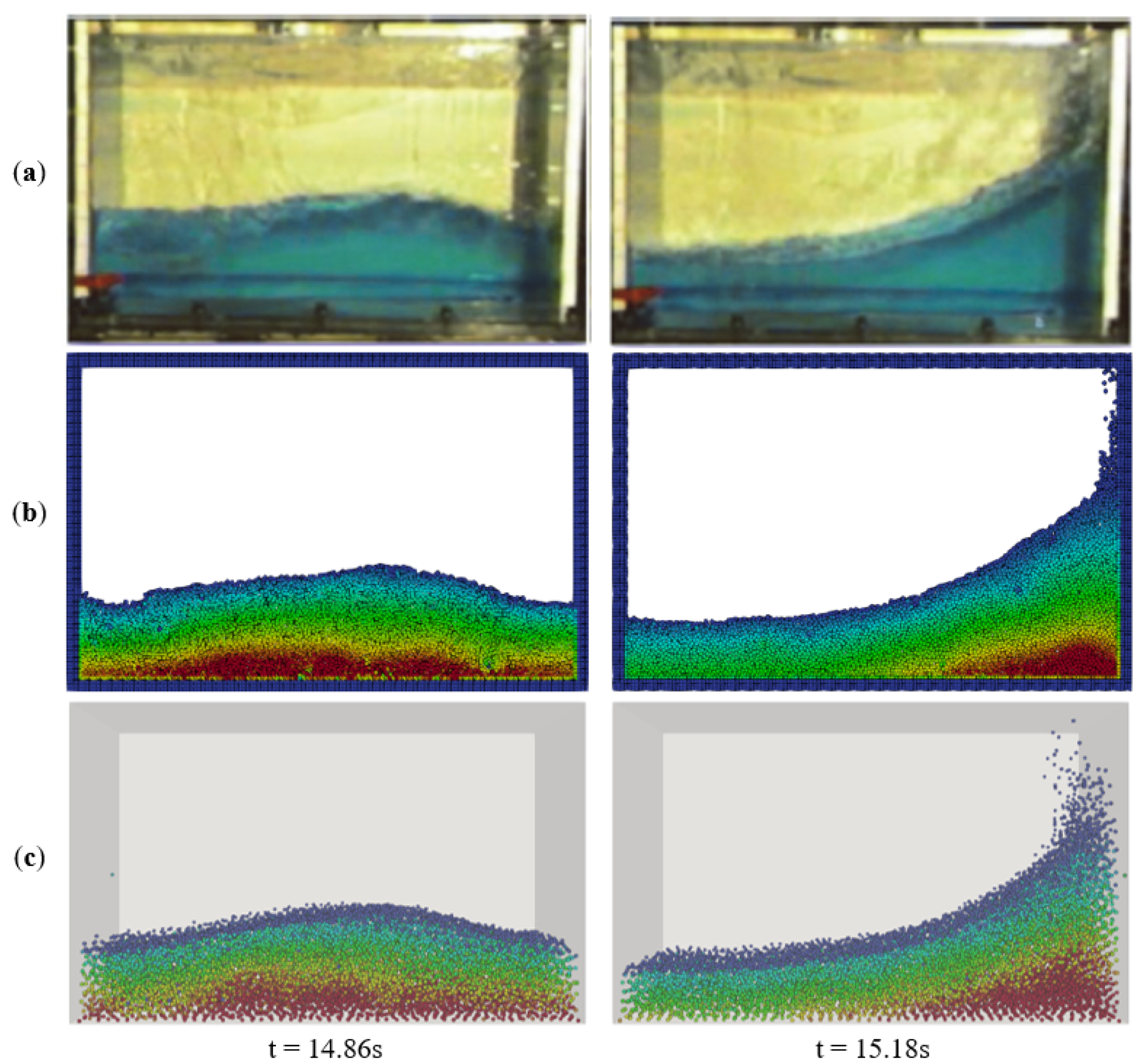
Comparisons of the numerical simulation results of the free surface profiles at time 14.86 s and 15.18 s with that of the experiments given by [60] are illustrated in Figure 3. From this figure, it can be seen that both the 2D and the 3D numerical simulation results make good agreement with the experimental results.

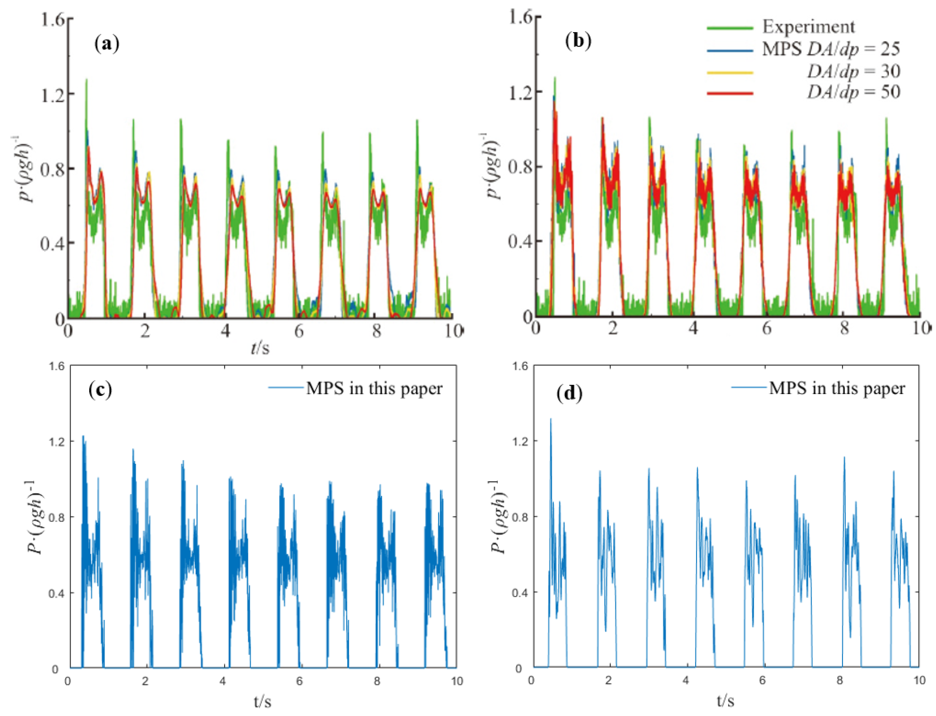
Meanwhile, comparisons of numerical simulation results of the pressure impact at the probe $P_0$ with that given by the experiments [60] and that given by another numerical simulation [52] are shown in Figure 4. From this figure, it can be seen that both 2D and 3D numerical simulation results obtained in this paper are in good agreement with that given by experimental results and numerical results. Despite few deviations in the 3D results, they all have almost the same maximum and minimum values and the same trend of the pressure.

The above numerical simulation results show that the MPS method used in this paper is effective in computing the dynamic pressure caused by the liquid sloshing in tanks swaying harmonically and thus can be used to numerically study the sloshing-induced force of ship tanks.

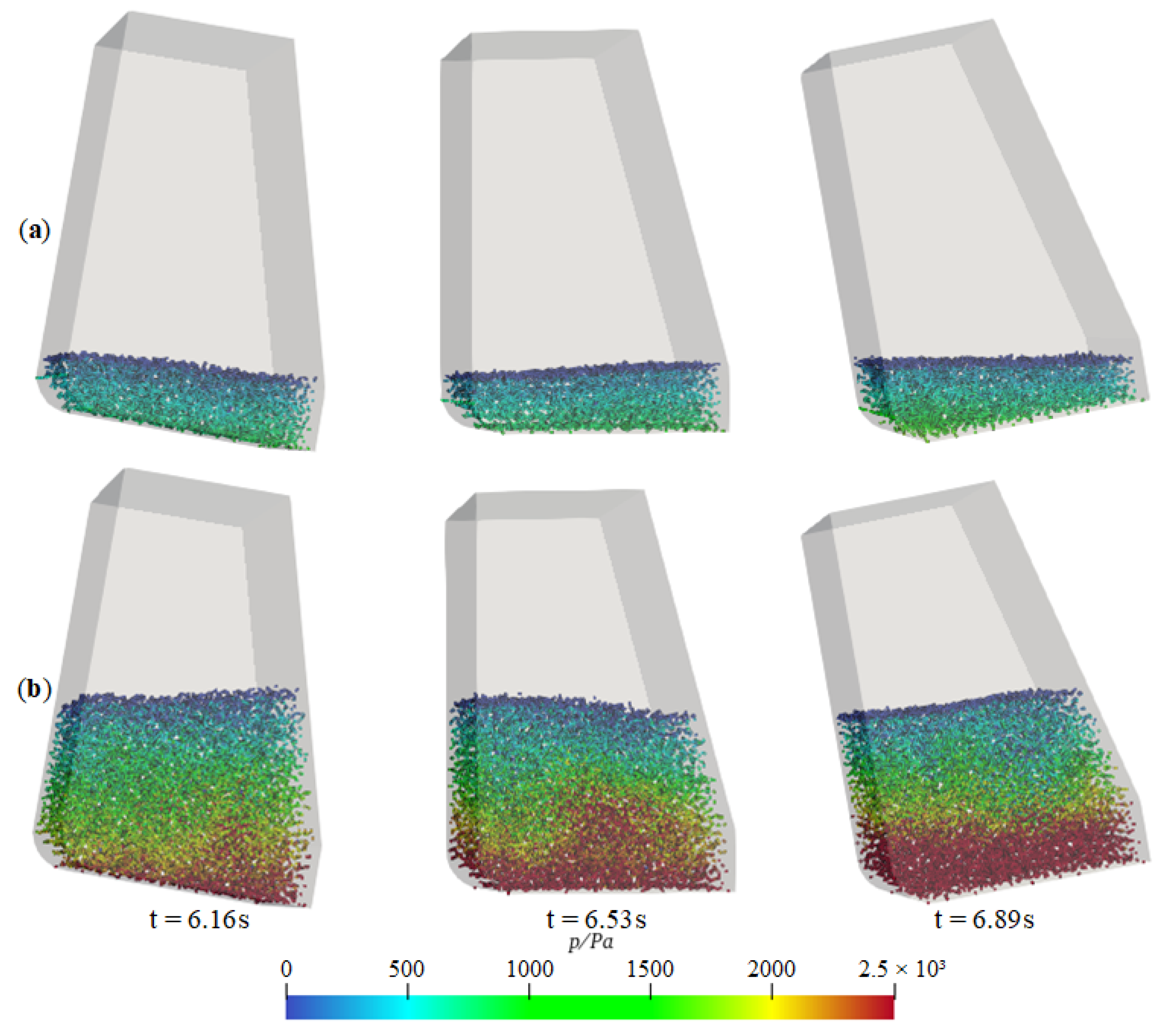
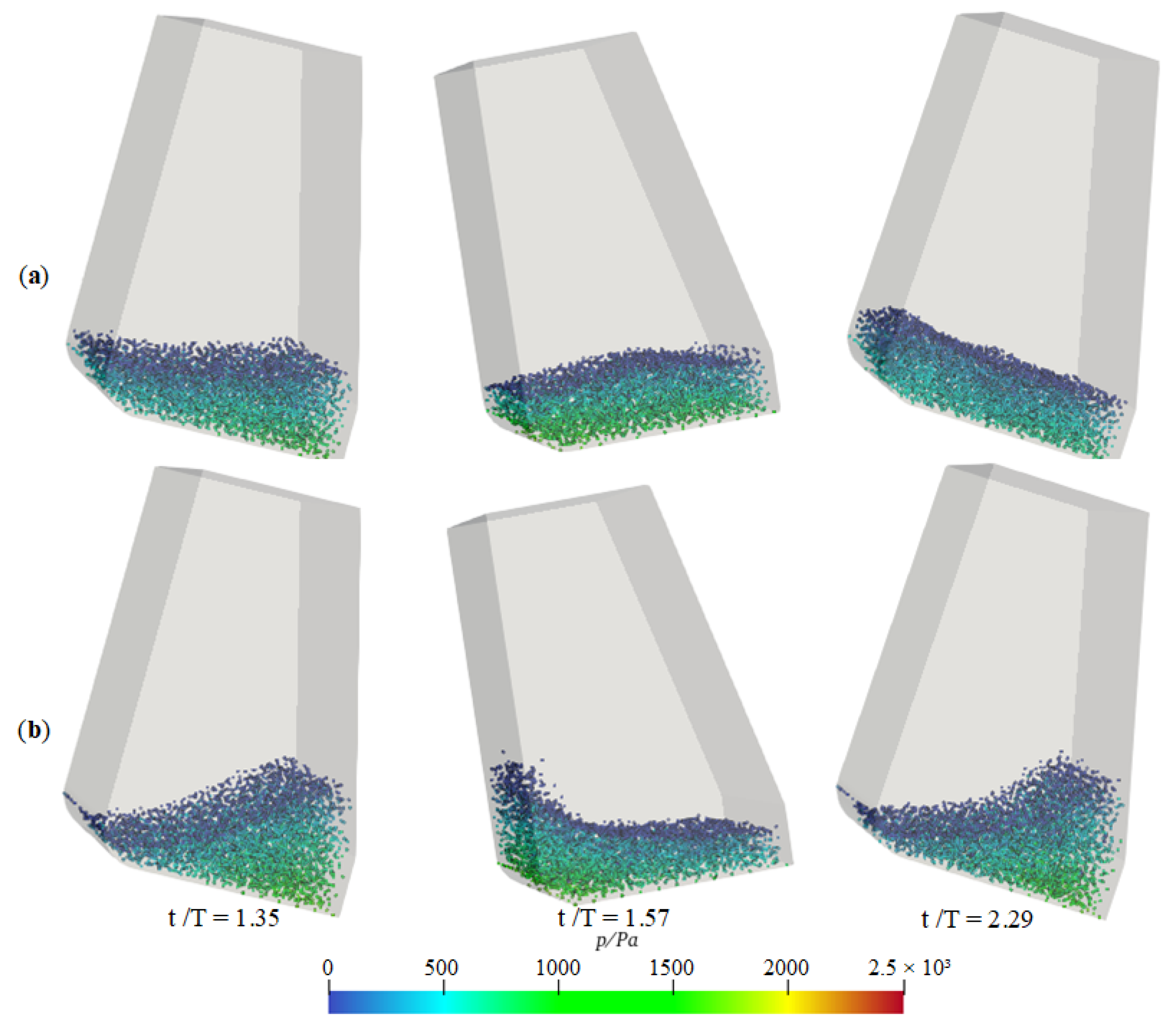
4. Numerical Results

4.1. Description of Test Cases

In this paper, numerical simulations of liquid sloshing are performed on a 400,000 DWT Very Large Ore Carrier (VLOC) “PACIFIC VISION”, which is designed by the Shanghai Merchant Ship Design and Research Institute (SDARI). Since liquid sloshing is mostly taking place in water ballast tanks, a ballast water tank of this VLOC, namely “R2.03AP”, is selected to carry out the numerical simulation of liquid sloshing in ship tanks under different rolling motions.

The principal particulars of “PACIFIC VISION” and the parameters of the water ballast tank “R2.03AP” are shown in

Table 1. Principal particulars of ‘PACIFIC VISION’, from [61].

Description	Value
Length overall	$361.90$ m
Length between perpendiculars (L.B.P.)	$355.00$ m
Breadth moulded	$65.00$ m
Depth moulded	$30.40$ m
Scantling draft moulded	$23.00$ m
Deadweight at scantling draft	$398,411.1$ t

and

Table 2. Parameters of the water ballast tank “R2.03AP”, from [61].

Description	Value
Compartment ident	R2.03AP
Volume	$8477.14$ m${}^3$
Aft end at frame	$117.00$ ($222.24$ m)
Fore end at frame	$123.00$ ($238.38$ m)
Lowest point	$0.00$ m above BL
Highest point	$30.97$ m above BL

, respectively [61]. The 3D design models of the hull and this water ballast tank are illustrated in Figure 5.

It is worth noting that a scaled model of “R2.03AP” is applied to carry out the simulation due to the limitation of computing ability. The scale ratio is set to 1:50. Meanwhile, five particular points on the port sidewall are selected to analyze the sloshing-induced pressure, as illustrated in Figure 6. It can be seen from the lateral view that, when the liquid level is low, the arc structure on the side away from the y-axis can effectively reduce the liquid impact. When the liquid level is high, the free surface area will decrease due to the slope of the bulkhead near the y-axis. The numerical simulation in the ship tanks can reflect the sloshing phenomena more realistically than the rectangular and other simplified tanks. The parameters of the scaled model and the particular points are shown in

Table 3. Parameters of the scale model of “R2.03AP” and the particular points.

Description	Value [mm]
Size of scale model in the x-direction	$322.80$
Size of scale model in the y-direction	$403.60$
Size of scale model in the z-direction	$619.48$
Height of Probe $P_1$ (above tank bottom)	$20.0$
Height of Probe $P_2$ (above tank bottom)	$80.0$
Height of Probe $P_3$ (above tank bottom)	$140.0$
Height of Probe $P_4$ (above tank bottom)	$200.0$
Height of Probe $P_5$ (above tank bottom)	$260.0$

.

One characteristic ballast load condition, LOADA02, is used to carry out numerical simulation. Parameters of “PACIFIC VISION” under this load condition are shown in

Table 4. Parameters of “PACIFIC VISION” under load condition LOADA02, from [61].

Draft	Trim	Displacement	T.C.G.	V.C.G.	GM
[m]	[m]	[t]	[m]	[m]	[m]
14.001	−0.149	260,089.5	0.059	15.342	17.27

, in which the terms “T.C.G.” and “V.C.G.” indicate the center of gravity of the ship of the breadth from the centerline and the height above the base line, respectively, and “GM” is ship’s metacentric height.

The undamped natural period of the ship $T_r$ can be determined by Equation [62], as follows:

$$T_r=\frac{2cB}{\sqrt{GM}}$$

(12)

where B is ship’s breadth moulded; and c is the coefficient describing ship’s transverse gyration radius, and is determined by:

$$c=0.373+0.023\frac{B}{T}-0.043\frac{L}{100}$$

(13)

where L and T is ship’s length between perpendiculars and mean ship draft, respectively.

In order to describe ship’s real motion, the dimensionless excitation period of the scaled tank and the real ship should be set to the same value. According to [63], the excitation period of the scaled tank $T_m$ can be determined by:

$$T_m·\sqrt{\frac{g}{H_m}}=T_r·\sqrt{\frac{g}{H_r}}$$

(14)

where g is the gravitational acceleration; and $H_m$:$H_r$ is the scaled ratio, which is set to 1:50 in this paper.

In this paper, the sloshing-induced dynamic force is numerically computed in four characteristic cases, which are the combinations of different filling ratio, maximum rolling angle, and rolling period, as described in

Table 5. Description of the numerically computation cases.

ID	Filling Height	Filling Ratio	Rolling Angle	Period
	[mm]	[%]	[${}^{\circ }$]	[s]
1	100	18.8	10	1.45 s
2	300	54.5	10	1.45 s
3	100	18.8	20	1.45 s
4	100	18.8	20	1.80 s

. It should also be noted that two different rolling periods are adopted to carry out numerical simulation. The first one, $1.45$ s, is obtained by Equations (12)–(14) and thus is the ship’s undamped natural period under the LOADA02 condition. The other one, $1.80$ s, is selected to simulate a more violent sloshing phenomenon. Meanwhile, the main calculation parameters used in the MPS method are described in

Table 6. Main calculation parameters used in the MPS method.

Parameters	Value
Initial particle spacing, $l_0$	$0.015$ m
Operating distance of Gradient model, $r_{Grad}$	$2.1$$l_0$
Operating distance of Laplacian model, $r_{Lap}$	$3.1$$l_0$
Time step size, $\Delta t$	$0.0005$ s
Density of fluid, $\rho$	1000 kg/m${}^3$
Free surface coefficient, $\beta$	$0.97$
Blending parameter, $\gamma$	$0.01$

.

All the cases have been performed in an Intel (R) Core (TM) i7-11700F 2.5 GHz single processor machine. The step size of the simulation is $5\times {10}^{-4}$ s. The relationship among the number of particles, computation time, and performed time steps for each case is shown in

Table 7. The relationship among the number of particles, computation time, and step size in all cases.

ID	Number of	Number of	Performed Time	Total Computational
	Fluid Particle	Boundary Particle	Step	Time
1	3696	22,013	15,000	4.2 h
2	10,290	23,289	15,000	13.3 h
3	3696	22,013	29,000	10.5 h
4	3696	22,013	36,000	13.0 h

.

4.2. Snapshots of Flow Field

The snapshots of flow field at several typical time steps under different filling ratio, maximum rolling angle, and rolling period are illustrated in Figure 7, Figure 8 and Figure 9.

Figure 7 gives the comparison of snapshots at several typical time steps under case 1 and case 2. Both of these cases have the same rolling period, 1.45 s, and maximum rolling angle, ${10}^{\circ }$, but different filling heights. The filling height in case 1 is 100 mm, while 300 mm in case 2. From this figure, it can be seen obviously that the profiles of free surface under these two cases are different, especially at time 6.53 s. This phenomenon is reasonable since the sloshing periods of the liquid in these two cases are different due to different filling height.

Figure 8 gives the comparison of snapshots at several typical time steps under case 1 and case 3. Both of these cases have the same rolling period, 1.45 s, and filling height is 100 mm, but different maximum rolling angles. The maximum rolling angle in case 1 is ${10}^{\circ }$, while ${20}^{\circ }$ in case 3. From this figure, it can be seen that the phenomenon of fluid accumulation, bending, and slamming on a free surface occurs in case 3, but not in case 1. Therefore, it can be concluded that a larger rolling angle would induce a more violent liquid sloshing in the ship tank.

Figure 9 gives the comparison of snapshots at several typical dimensionless time steps under case 3 and case 4. Both of these cases have same maximum rolling angle, ${20}^{\circ }$, and filling height, 100 mm, but different rolling periods. The rolling period in case 3 is $1.45$ s, while $1.8$ s in case 4. From this figure, it can be seen that, although the phenomenon of fluid accumulation, bending and slamming on free surface occurs in these two cases, the liquid sloshing in case 4 is more violent than that in case 3. This difference can be explained by the fact that the sloshing intensity of the liquid in sloshing tanks is not positively correlated with the ship’s undamped natural rolling frequency.

From Figure 7, Figure 8 and Figure 9, it can also be seen that the movement of the free surface, like the phenomena of fluid accumulation, bending and slamming, occurs in the sloshing tank. This proves that the traditional quasi-static method, assuming the free surface is parallel to the sea level, cannot reflect sloshing phenomena realistically.

4.3. Pressure and Force

Figure 10 gives the comparison of hydrostatic pressure with the dynamic pressure at three particular points, namely $P_2$, $P_3$, and $P_4$, in case 2. It should be noted that the method is adopted to determine the height of the liquid surface of the tank under different ships’ rolling angles to calculate the hydrostatic pressure [64]. From this figure, it can be seen that the maximum dynamic pressure is bigger than hydrostatic pressure in all three of these points, even 38% at $P_4$.

Figure 11 gives the comparison of dynamic pressure at two particular points in two cases, namely case 1 and case 3. From this figure, it can be seen that the curve of the dynamic pressure in case 3 (red curve) is higher than the curve in case 1 (green curve), which demonstrates that a larger rolling angle would induce a bigger dynamic pressure.

When setting the solid particles on a sidewall, the sidewall is actually discretized with a uniform grid. Thus, the sloshing-induced pressure at each cell could be obtained by the pressure of the corresponding particle. After that, the sloshing-induced force on the sidewall can be calculated by integration [65], as follows:

$$F=\sum _{t=1}^N{P}_i(\Delta z_i·W_i)$$

(15)

where $P_i$ is the sloshing-induced pressure at the i-th particle on the sidewall; $\Delta z_i$ and $W_i$ are the height and length of the i-th cell, respectively. In this paper, both $\Delta z_i$ and $W_i$ are equal to the initial space between solid particles.

Figure 12 gives the comparison of the sloshing-induced forces on the port sidewall of the tank in case 3 with that in case 4. In addition, the hydrostatic force is marked as a red dash line. From this figure, it can be seen that the peaks of sloshing-induced force in both cases are bigger than hydrostatic force, even 20% in case 4. Furthermore, the maximum sloshing-induced force in case 4 is larger than that in case 3. These results can also be seen by the fact that the high pressure area in case 4 is wider than that in case 3, as illustrated in Figure 9. Meanwhile, a bigger sloshing-induced force would be expected when liquid sloshing is more violent since the liquid sloshing in case 4 is more violent than in case 3. Therefore, it could claim that the sloshing-induced force is not positively correlated with the ships’ undamped natural rolling frequency.

5. Conclusions

This paper lays a solid foundation for further research on the effect of tank sloshing on the dynamic stability of ships. The phenomena of liquid sloshing in a ballast tank under realistic ship rolling motion are numerically simulated by using the MPS method. After that, sloshing-induced force on sidewall of the tank is obtained and analyzed.

Conclusions can be summarized as follows:

(1) The phenomena of large deformation and nonlinear fragmentation of free surface, e.g., accumulation, bending and slamming, etc., can be found in liquid sloshing, which proves that a traditional quasi-static method cannot reflect the influence of the violent free surface on ship dynamic stability. In this case, meshfree methods should be used to get more realistic results.

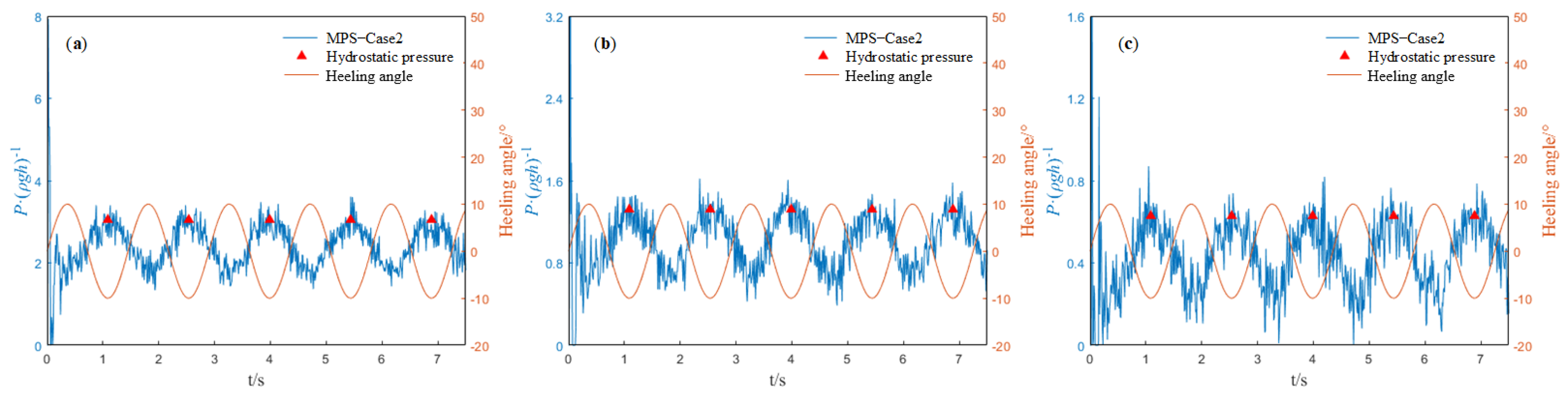
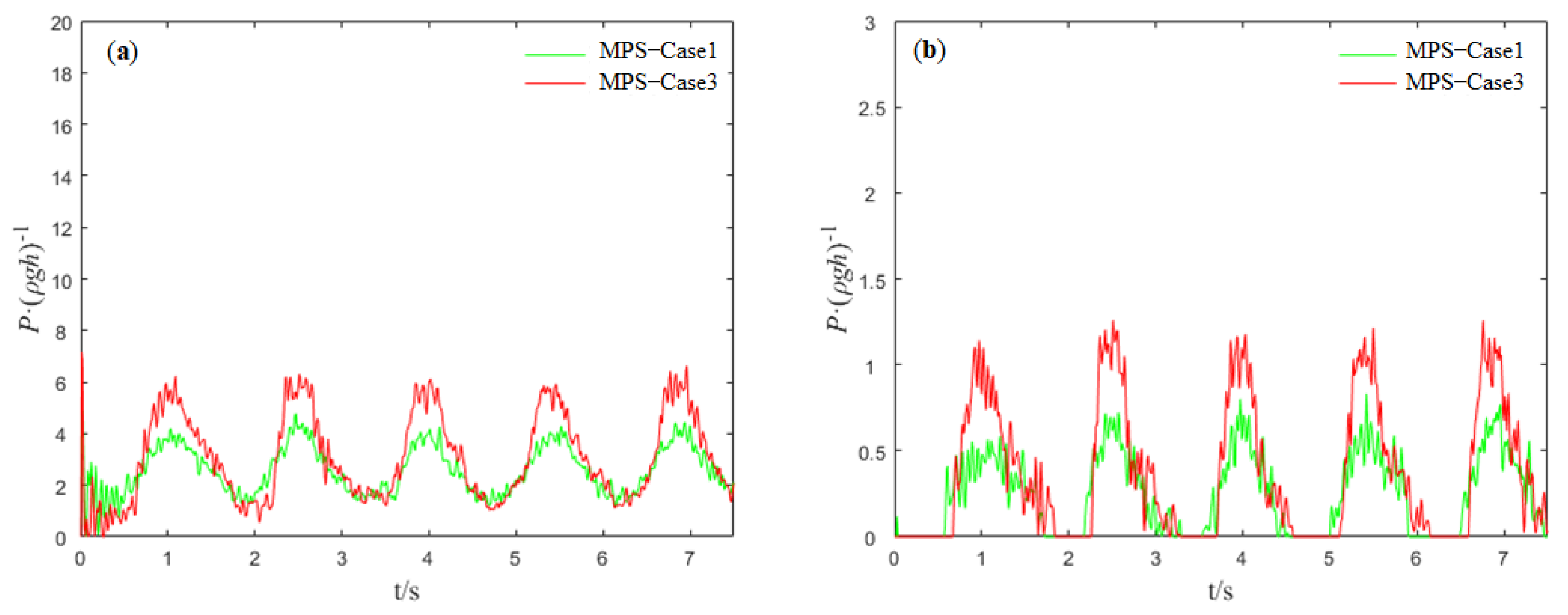
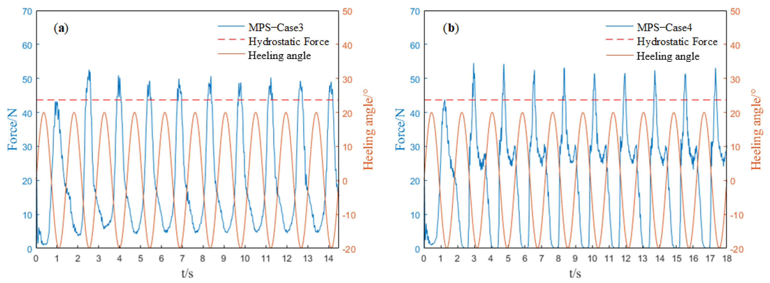
(2) The maximum sloshing-induced force is much bigger than the corresponding static one, e.g., 20% bigger in some cases. Meanwhile, both the rolling angle and period have significant effects on liquid sloshing. The sloshing intensity of the liquid in sloshing tanks is not positively correlated with the ship’s undamped natural rolling frequency.

(3) A large number of numerical simulations of liquid sloshing through a series of different ships’ undamped natural periods can be carried out. The relationship between the rolling periods and the liquid filling rates of the most violent liquid sloshing will be investigated. By establishing the database of this relationship, it can provide effective suggestions for ship operators, such as changing the ballast water to adjust the dynamic stability of the ship.

Although the MPS method has its own advantages, it also has the limitation of computing ability in dealing with large-scale violent free surface flow. This is the reason why this paper uses a scaled tank model to perform the simulation. Therefore, a more effective MPS method should be further investigated to simulate the liquid sloshing in all ship tanks of real size simultaneously.

References

1. Chen, B.F.; Wu, C.H. Effects of excitation angle and coupled heave–surge–sway motion on fluid sloshing in a three-dimensional tank. J. Mar. Sci. Technol. 2011, 16, 22–50. [Google Scholar] [CrossRef]
2. Wang, J.H.; Sun, S.L. Study on liquid sloshing characteristics of a swaying rectangular tank with a rolling baffle. J. Eng. Math. 2019, 119, 23–41. [Google Scholar] [CrossRef] [Green Version]
3. Du, Y.; Wang, C.X.; Zhang, N. Numerical simulation on coupled ship motions with nonlinear sloshing. Ocean Eng. 2019, 178, 493–500. [Google Scholar] [CrossRef]
4. Bredmose, H.; Brocchini, M.; Peregrine, D.H.; Thais, L. Experimental investigation and numerical modelling of steep forced water waves. J. Fluid Mech. 2003, 490, 217. [Google Scholar] [CrossRef]
5. Kim, Y.; Shin, Y.S.; Lee, K.H. Numerical study on slosh-induced impact pressures on three-dimensional prismatic tanks. Appl. Ocean Res. 2004, 26, 213–226. [Google Scholar] [CrossRef]
6. Kim, Y.; Nam, B.W.; Kim, D.W.; Kim, Y.S. Study on coupling effects of ship motion and sloshing. Ocean Eng. 2007, 34, 2176–2187. [Google Scholar] [CrossRef]
7. Buldakov, E. Lagrangian modelling of fluid sloshing in moving tanks. J. Fluids Struct. 2014, 45, 1–14. [Google Scholar] [CrossRef] [Green Version]
8. Saghi, H. A parametric study on wave–floating storage tank interaction using coupled VOF-FDM method. J. Mar. Sci. Technol. 2019, 24, 454–465. [Google Scholar] [CrossRef]
9. Sriram, V.; Sannasiraj, S.A.; Sundar, V. Numerical simulation of 2D sloshing waves due to horizontal and vertical random excitation. Appl. Ocean Res. 2006, 28, 19–32. [Google Scholar] [CrossRef]
10. Belakroum, R.; Kadja, M.; Mai, T.H.; Maalouf, C. An efficient passive technique for reducing sloshing in rectangular tanks partially filled with liquid. Mech. Res. Commun. 2010, 37, 341–346. [Google Scholar] [CrossRef]
11. Wang, W.Y.; Peng, Y.; Zhang, Q.; Ren, L.; Jiang, Y. Sloshing of liquid in partially liquid filled toroidal tank with various baffles under lateral excitation. Ocean Eng. 2017, 146, 434–456. [Google Scholar] [CrossRef]
12. Amano, Y.; Ishikawa, S.; Yoshitake, T.; Kondou, T. Modeling and design of a tuned liquid damper using triangular-bottom tank by a concentrated mass model. Nonlinear Dyn. 2021, 104, 1917–1935. [Google Scholar] [CrossRef]
13. Lee, D.H.; Kim, M.H.; Kwon, S.H.; Kim, J.W.; Lee, Y.B. A parametric sensitivity study on LNG tank sloshing loads by numerical simulations. Ocean Eng. 2007, 34, 3–9. [Google Scholar] [CrossRef]
14. Jiang, S.C.; Teng, B.; Bai, W.; Gou, Y. Numerical simulation of coupling effect between ship motion and liquid sloshing under wave action. Ocean Eng. 2015, 108, 140–154. [Google Scholar] [CrossRef]
15. Yang, C.; Niu, R.; Zhang, P. Numerical analyses of liquid slosh by Finite volume and Lattice Boltzmann methods. Aerosp. Sci. Technol. 2021, 113, 106681. [Google Scholar] [CrossRef]
16. Ding, S.F.; Wang, G.; Luo, Q.M. Study on sloshing simulation in the independent tank for an ice-breaking LNG carrier. Int. J. Nav. Archit. Ocean Eng. 2020, 12, 667–679. [Google Scholar] [CrossRef]
17. Kim, D. Potential solution for sloshing in a horizontally moving rectangular tank and design of tank velocity profile. J. Mech. Sci. Technol. 2021, 35, 2981–2988. [Google Scholar] [CrossRef]
18. He, T.; Feng, D.K.; Liu, L.W.; Wang, X.Z.; Jiang, H. CFD Simulation and Experimental Study on Coupled Motion Response of Ship with Tank in Beam Waves. J. Mar. Sci. Eng. 2022, 10, 113. [Google Scholar] [CrossRef]
19. Chen, X.; Wan, D.C. GPU accelerated MPS method for large-scale 3D violent free surface flows. Ocean Eng. 2019, 171, 677–694. [Google Scholar] [CrossRef]
20. Liu, M.B.; Liu, G.R. Smoothed particle hydrodynamics (SPH): An overview and recent developments. Arch. Comput. Methods Eng. 2010, 17, 25–76. [Google Scholar] [CrossRef] [Green Version]
21. Gingold, R.A.; Monaghan, J.J. Smoothed particle hydrodynamics: Theory and application to non-spherical stars. Mon. Not. R. Astron. Soc. 1977, 181, 375–389. [Google Scholar] [CrossRef]
22. Lucy, L.B. A numerical approach to the testing of the fission hypothesis. Astron. J. 1977, 82, 1013–1024. [Google Scholar] [CrossRef]
23. Monaghan, J.J. Simulating free surface flows with SPH. J. Comput. Phys. 1994, 110, 399–406. [Google Scholar] [CrossRef]
24. Iglesias, A.S.; Rojas, L.P.; Rodríguez, R.Z. Simulation of anti-roll tanks and sloshing type problems with smoothed particle hydrodynamics. Ocean Eng. 2004, 31, 1169–1192. [Google Scholar] [CrossRef]
25. Souto, I.A.; Delorme, L.; Pérez-Rojas, L.; Abril-Pérez, S. Liquid moment amplitude assessment in sloshing type problems with smooth particle hydrodynamics. Ocean Eng. 2006, 33, 1462–1484. [Google Scholar] [CrossRef]
26. Colagrossi, A.; Antuono, M.; Le Touzé, D. Theoretical considerations on the free-surface role in the smoothed-particle-hydrodynamics model. Phys. Rev. E 2009, 79, 056701. [Google Scholar] [CrossRef]
27. Gomez-Gesteira, M.; Rogers, B.D.; Dalrymple, R.A.; Crespo, A.J. State-of-the-art of classical SPH for free-surface flows. J. Hydraul. Res. 2010, 48, 6–27. [Google Scholar] [CrossRef]
28. Bouscasse, B.; Antuono, M.; Colagrossi, A.; Lugni, C. Numerical and experimental investigation of nonlinear shallow water sloshing. Int. J. Nonlinear Sci. Numer. Simul. 2013, 14, 123–138. [Google Scholar] [CrossRef]
29. Gotoh, H.; Khayyer, A.; Ikari, H.; Arikawa, T.; Shimosako, K. On enhancement of Incompressible SPH method for simulation of violent sloshing flows. Appl. Ocean Res. 2014, 46, 104–115. [Google Scholar] [CrossRef]
30. Green, M.D.; Peiró, J. Long duration SPH simulations of sloshing in tanks with a low fill ratio and high stretching. Comput. Fluids 2018, 174, 179–199. [Google Scholar] [CrossRef]
31. Hu, T.A.; Wang, S.Q.; Zhang, G.Y.; Sun, Z.; Zhou, B. Numerical simulations of sloshing flows with an elastic baffle using a SPH-SPIM coupled method. Appl. Ocean Res. 2019, 93, 101950. [Google Scholar] [CrossRef]
32. Li, J.P.; Cao, D.J.; Pan, K. Dry-friction-induced self-excitation of a rectangular liquid-filled tank. Nonlinear Dyn. 2020, 102, 1337–1359. [Google Scholar] [CrossRef]
33. Tao, K.D.; Zhou, X.Q.; Ren, H.L. A Novel Improved Coupled Dynamic Solid Boundary Treatment for 2D Fluid Sloshing Simulation. J. Mar. Sci. Eng. 2021, 9, 1395. [Google Scholar] [CrossRef]
34. Zhang, Z.L.; Khalid, M.; Long, T.; Liu, M.B.; Shu, C. Improved element-particle coupling strategy with δ-SPH and particle shifting for modeling sloshing with rigid or deformable structures. Appl. Ocean Res. 2021, 114, 102774. [Google Scholar] [CrossRef]
35. Koshizuka, S.; Shibata, K.; Kondo, M.; Matsunaga, T. Moving Particle Semi-Implicit Method: A Meshfree Particle Method for Fluid Dynamics, 1st ed.; Academic Press: London, UK, 2018; pp. 162–168. [Google Scholar]
36. Koshizuka, S.; Oka, Y. Moving-particle semi-implicit method for fragmentation of incompressible fluid. Nucl. Sci. Eng. 1996, 123, 421–434. [Google Scholar] [CrossRef]
37. Lee, B.H.; Park, J.C.; Kim, M.H.; Hwang, S.C. Step-by-step improvement of MPS method in simulating violent free-surface motions and impact-loads. Comput. Methods Appl. Mech. Eng. 2011, 200, 1113–1125. [Google Scholar] [CrossRef]
38. Kakuda, K.; Obara, S.; Toyotani, J.; Meguro, M.; Furuichi, M. Fluid flow simulation using particle method and its physics-based computer graphics. Comput. Model. Eng. Sci. 2012, 83, 57–72. [Google Scholar]
39. Zhang, Y.X.; Wan, D.C. Numerical simulation of liquid sloshing in low-filling tank by MPS. Chin. J. Hydrodyn. 2012, 27, 100–107. [Google Scholar]
40. Khayyer, A.; Gotoh, H. A higher order Laplacian model for enhancement and stabilization of pressure calculation by the MPS method. Appl. Ocean Res. 2010, 32, 124–131. [Google Scholar] [CrossRef]
41. Wu, Q.R.; Tan, M.Y.; Xing, J.T. An improved moving particle semi-implicit method for dam break simulation. J. Ship Mech. 2014, 18, 1044–1054. [Google Scholar]
42. Khayyer, A.; Gotoh, H. Enhancement of stability and accuracy of the moving particle semi-implicit method. J. Comput. Phys. 2011, 230, 3093–3118. [Google Scholar] [CrossRef]
43. Jena, D.; Biswal, K.C. A numerical study of violent sloshing problems with modified MPS method. J. Hydrodyn. 2017, 29, 659–667. [Google Scholar] [CrossRef]
44. Wang, L.Z.; Khayyer, A.; Gotoh, H.; Jiang, Q.; Zhang, C.K. Enhancement of pressure calculation in projection-based particle methods by incorporation of background mesh scheme. Appl. Ocean Res. 2019, 86, 320–339. [Google Scholar] [CrossRef]
45. Xiao, H.W.; Jin, Y.C. Development of explicit moving particle simulation method with applications. Comput. Fluids 2022, 235, 105270. [Google Scholar] [CrossRef]
46. Tanaka, M.; Masunaga, T. Stabilization and smoothing of pressure in MPS method by quasi-compressibility. J. Comput. Phys. 2010, 229, 4279–4290. [Google Scholar] [CrossRef]
47. Daneshvar, F.A.; Rakhshandehroo, G.R.; Talebbeydokhti, N. New modified gradient models for MPS method applied to free-surface flow simulations. Appl. Ocean Res. 2017, 66, 95–116. [Google Scholar] [CrossRef]
48. Wang, C.H.; Guo, C.Y.; Han, F.L. LNG Tank Sloshing Simulation of Multidegree Motions Based on Modified 3D MPS Method. Math. Probl. Eng. 2020, 2020, 4018925. [Google Scholar] [CrossRef]
49. Zhang, G.Y.; Zhao, W.W.; Wan, D.C. Numerical simulations of sloshing waves in vertically excited square tank by improved MPS method. J. Hydrodyn. 2022, 34, 76–84. [Google Scholar] [CrossRef]
50. Zhang, Y.X.; Wan, D.C.; Takanori, H. Comparative study of MPS method and level-set method for sloshing flows. J. Hydrodyn. Ser. B 2014, 26, 577–585. [Google Scholar] [CrossRef]
51. Chen, X.; Wan, D.C. Numerical simulation of three-dimensional violent free surface flows by GPU-based MPS method. Int. J. Comput. Methods 2019, 16, 1843012. [Google Scholar] [CrossRef]
52. Xie, F.Z.; Zhao, W.W.; Wan, D.C. CFD simulations of three-dimensional violent sloshing flows in tanks based on MPS and GPU. J. Hydrodyn. 2020, 32, 672–683. [Google Scholar] [CrossRef]
53. Jandaghian, M.; Krimi, A.; Zarrati, A.R.; Shakibaeinia, A. Enhanced weakly-compressible MPS method for violent free-surface flows: Role of particle regularization techniques. J. Comput. Phys. 2021, 434, 110202. [Google Scholar] [CrossRef]
54. Wang, L.Z.; Xu, M.; Zhang, Q. Numerical Investigation of Shallow Liquid Sloshing in a Baffled Tank and the Associated Damping Effect by BM-MPS Method. J. Mar. Sci. Eng. 2021, 9, 1110. [Google Scholar] [CrossRef]
55. Felix-Gonzalez, I.; Sanchez-Mondragon, J.; Cruces-Giron, A.R. Sloshing study on prismatic LNG tank for the vertical location of the rotational center. Comput. Part. Mech. 2022, 1, 1–20. [Google Scholar] [CrossRef]
56. aus der Wiesche, S. Sloshing dynamics of a viscous liquid in a spinning horizontal cylindrical tank. Aerosp. Sci. Technol. 2008, 12, 448–456. [Google Scholar] [CrossRef]
57. Zhang, G.Y.; Wu, J.X.; Sun, Z.; el Moctar, O.; Zong, Z. Numerically simulated flooding of a freely-floating two-dimensional damaged ship section using an improved MPS method. Appl. Ocean Res. 2020, 101, 102207. [Google Scholar] [CrossRef]
58. Koshizuka, S.; Oka, Y. Moving particle semi-implicit method: Fully lagrangian analysis of incompressible flows. In Proceedings of the European Congress on Computational Methods in Applied Sciences and Engineering (ECCOMAS), Barcelona, Spain, 11–14 September 2000. [Google Scholar]
59. Zhu, X.S.; Cheng, L.; Lu, L.; Teng, B. Implementation of the moving particle semi-implicit method on GPU. Sci. China Phys. Mech. Astron. 2011, 54, 523–532. [Google Scholar] [CrossRef]
60. Kang, D.H.; Lee, Y.B. Summary Report of Sloshing Model Test for Rectangular Model; Daewoo Shipbuilding & Marine Engineering Co., Ltd.: Gyeongnam, Korea, 2019. [Google Scholar]
61. SDARI. Final Loading Manual of 400,000 DWT Ore Carrier “PACIFIC VISION”; Shanghai Merchant Ship Design and Research Institute: Shanghai, China, 2019. [Google Scholar]
62. Wawrzyński, W.; Krata, P. Method for ship’s rolling period prediction with regard to nonlinearity of GZ curve. J. Theor. Appl. Mech. 2016, 54, 1329–1343. [Google Scholar] [CrossRef] [Green Version]
63. Tan, Q.M. Dimensional Analysis, 1st ed.; Springer: Berlin/Heidelberg, Germany, 2011; pp. 7–16. [Google Scholar]
64. Sun, X.F.; Ni, Y.G.; Liu, C.L.; Wang, Z.Z.; Yin, Y. A practical method for stability assessment of a damaged ship. Ocean Eng. 2021, 222, 108594. [Google Scholar] [CrossRef]
65. Chu, C.R.; Wu, Y.R.; Wu, T.R.; Wang, C.Y. Slosh-induced hydrodynamic force in a water tank with multiple baffles. Ocean Eng. 2018, 167, 282–292. [Google Scholar] [CrossRef]
Figure 1. Illustration of preprocessing.
Applsci 12 05130 g001
Figure 2. Flow chart of MPS numerical simulation.
Applsci 12 05130 g002
Figure 3. Comparisons of free surface profiles results. (a) experimental results given by [60]; (b) 2D numerical simulation results obtained in this paper; (c) 3D numerical simulation results obtained in this paper.
Applsci 12 05130 g003
Figure 4. Comparisons of numerical simulation results of the pressure impact at the probe P 0 . (a) 2D results given by [52,60]; (b) 3D results given by [52,60]; (c) 2D numerical simulation results of this paper; (d) 3D numerical simulation results of this paper.
Applsci 12 05130 g004
Figure 5. Illustration of the 3D design models of “PACIFIC VISION”.
Applsci 12 05130 g005
Figure 6. Illustration of the particular points on “R2.03AP”. (a) custom view; (b) lateral view.
Applsci 12 05130 g006
Figure 7. Snapshots of flow field in different filling ratios. (a) case 1; (b) case 2.
Applsci 12 05130 g007
Figure 8. Snapshots of flow field at different rolling angles. (a) case 1; (b) case 3.
Applsci 12 05130 g008
Figure 9. Snapshots of flow field in different rolling periods. (a) case 3; (b) case 4.
Applsci 12 05130 g009
Figure 10. Comparison between hydrostatic and dynamic pressure in case 2 at three probes. (a) P 2 ; (b) P 3 ; (c) P 4 .
Applsci 12 05130 g010
Figure 11. Comparison of dynamic pressure at different rolling angles in case 1 and case 3 at two probes. (a) P 1 ; (b) P 2 .
Applsci 12 05130 g011
Figure 12. Comparison of dynamic force at two rolling periods in case 3 and case 4. (a) case 3; (b) case 4.
Applsci 12 05130 g012