New Product Short-Term Demands Forecasting with Boxplot-Based Fractional Grey Prediction Model

Abstract

The cost of investing in new product development (NPD) is high, and it is a feasible way to use demand forecasts for customer or end-users as a decisive reference. However, this short-term time-series data has difficulties in learning because there is no past performance on which to base the estimates. In the past, it has been proven that the cumulative method of the fractional grey prediction model (FGM) is better than the traditional integer cumulative method of the grey model (GM) model. There are many studies using different optimal algorithms to determine the moderate score order. How to set the coefficient of α in FGM is also worth exploring. Therefore, this research reveals a new fractional grey prediction model which uses box-and-whisker plots to estimate the trends of data, known as the boxplot-based fractional scale prediction model (boxplot-based FGM, BP-FGM) to improve the accuracy of predictors by setting the coefficient sets of α. In the experiment, the examined dataset was collected from a well-known equipment manufacturer as the research object. For modeling, the mean absolute percentage error (MAPE) was established as the objective function of the optimization model, the results from three datasets verified the effect through the commodity attributes and public test data of its production, and the experimental results show that BP-FGM has better prediction results than FGM.

1. Introduction

In the equipment manufacturing industry of semiconductors and displays, the production environment is rigorous, life cycles are becoming shorter, and once the product has been reviewed and approved by the customer, the production is gradually increased. It is a severe challenge for the company to accurately predict the demand for extremely new products, because there is no large amount of historical sales data [1,2,3]. Therefore, how to accurately predict the demand for its products will be a serious challenge. How to find a reasonable demand prediction method is also worthy of further exploration.

Product diversification usually requires the shortening of the time for new product development (NPD) processes in order to accelerate the launch of prototypes to markets is the key to gaining more market shares. Moreover, data collected from the demand forecasting provides important resources for decision support to plan capacity and allocate the associated capital investments for capacity expansion, requiring a longer lead time. However, how to forecast sales demands for new and extremely new products is the greatest challenge due to lack of data [1,3].

The grey model (GM) was first proposed to deal with the issues concerning uncertainty and insufficient information form short-term time-series data [4]. It aims to make predictions based on few-shot datasets and is the foundation of grey system theory. The GM (1,1) model is the most common and basic model. The features include the low requirement of population data, is easily operated, and includes the low loading of calculations [5]. The main concept is to detect the underlying patterns from the collected data with an accumulated generating operation (AGO), which processes sample data indirectly [6]. The grey models based on the fractional order model (FGM) has been proven to be a better method than the traditional GM, while the fractional order-r value is set in a continuous real number space [7,8,9,10,11]. In the past, much research used heuristic optimization algorithms, such as genetic algorithms and particle swarm optimization, etc., to improve the accuracy of predictions [5,9,11,12,13,14]. In this paper, we focus on how to improve the FGM by revealing a new fractional grey prediction model, which uses box-and-whisker plots to estimate the trend of data, known as the box-plot-based fractional scale prediction model (boxplot-based FGM, BP-FGM), to improve the accuracy of predictors by setting the coefficient sets of background value α in a traditional grey model.

The following sections are organized as follows, the box-and-whisker plots theorem and grey system model are addressed in Section 2. Section 3 re-examines selected new product forecasting techniques, including fractional scale accumulation and optimization for background values. We also provided the discussion of the models presented in this research as the final section.

2. Literature Review

There are two topics introduced in this section, the box-and-whisker plots, grey system theory and the grey model in a fractional order.

2.1. Box-And-Whisker Plot

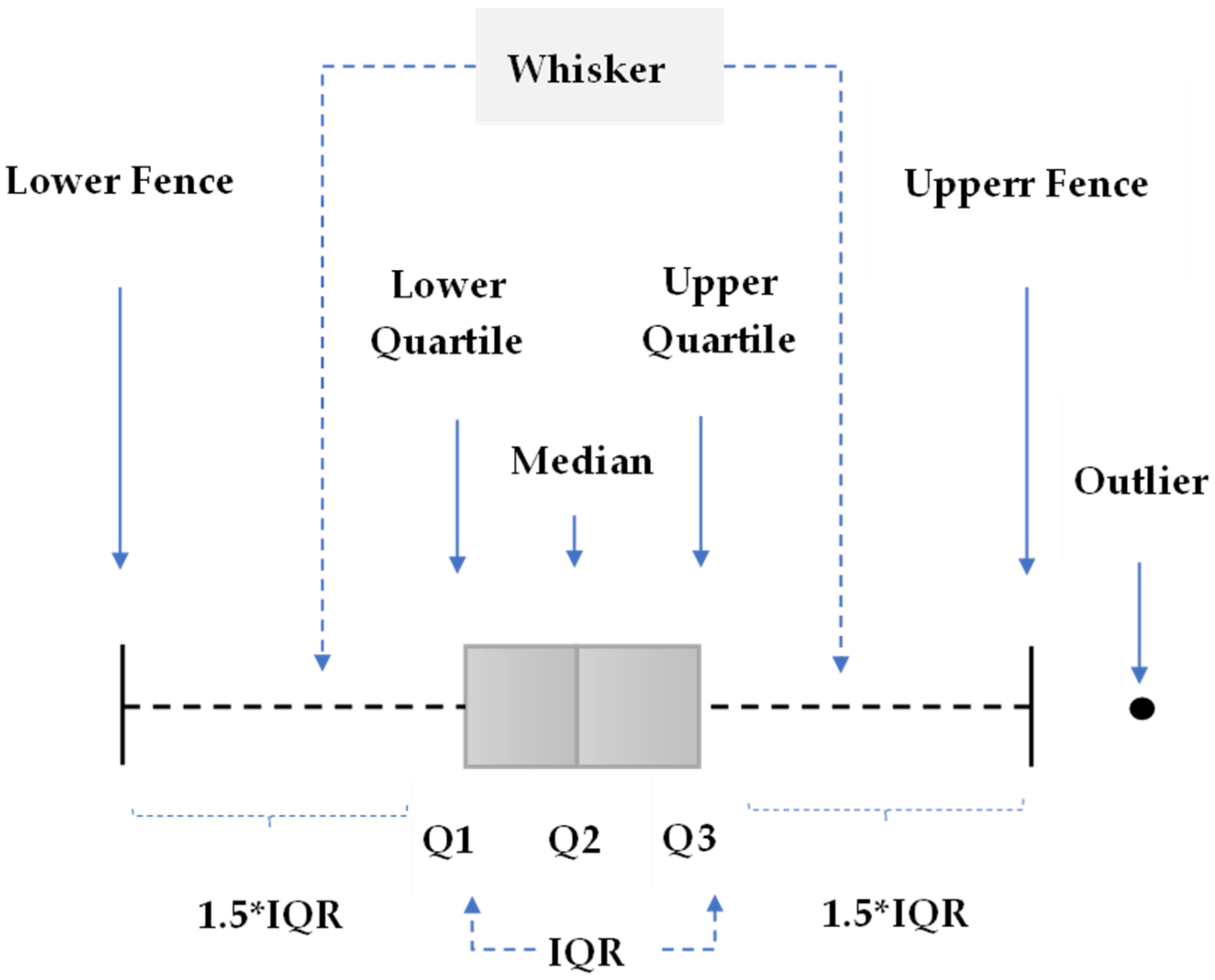
A box-and-whisker plot (or simply called a boxplot) is a method of visualizing the range of data, displaying the main data tendencies and of distributing symmetry and integrating the above information into a histogram-like chart in order to illustrate how values vary and concentrate with respect to a given data distribution [15].

When drawing a boxplot, five statistics are required: the minimum value, the 1st quartile (lower, Q1), the 2nd quartile (regarded as median, Q2), the 3rd quartile (upper, Q3) and the maximum value, which divide all the data into four equal parts, and each section includes approximately 25% of the values. The 1st quartile divides data into two groups, data with values lower than Q1 (25% of the data amount) and others (75% of the data amount). In the same way, the 2nd quartile divides data into the subset with values lower than Q2 and the subset with values larger than Q2; each subset contains an even half of the data amount, and so on for Q3. In terms of the form of a “boxplot”, the main feature is a rectangle that extends from the 1st quartile through to the 3rd quartile, i.e., the box’s length equals the interquartile range, and the range between Q1 and Q3, also named IQR [16].

The dash lines stretching from both the box’s sides are named the “whiskers”, used to indicate variability outside both quartiles. The corresponding lengths are obtained by $\mathrm{Q}1-1.5\times \mathrm{IQR}$ (lower fence) and $\mathrm{Q}3+1.5\times \mathrm{IQR}$ (upper fence). Typically, outliers are plotted as individual dots beyond the fences. Additionally, boxplots can be drawn either vertically or horizontally [16]. Figure 1 shows the horizontal form of a boxplot.

2.2. Grey System Model

Deng first proposed the grey model (GM) [4] in 1982. It aims to handle the issues concerned with uncertain and insufficient information in short-term time-series data. There is still room for improving the prediction accuracy by means of enhancing the basic theories in GM and setting the coefficients. Finding the suitable background values which determine the developing coefficient $\alpha$ and the grey input $b$ is another efficient way, where $\alpha$ is the growth factor and $b$ is a grey control parameter, the accuracy of the prediction models is rely on these two coefficients.

In GM (1,1), the newer data changes on the prediction model below the old data, which goes against the concept of the new data priority principle, thus limiting the scope of applying grey predictions. The theory of combining the cumulative generator of the fractional order with the grey prediction model, also named the grey system model, with the fractional order model (FGM), based on the new information priority principle [5], flattens the increase sequence by selecting the appropriate cumulative order, thereby increasing the accuracy of the prediction [7,8]. In the traditional FGM (1,1) model, the background value is formulated as:

$$z^{\left(r\right)}\left(\kappa \right)=\frac{1}{2}\left[x^{\left(r\right)}\left(k\right)+x^{\left(r\right)}\left(k-1\right)\right]$$

(1)

where $0<r\le 1$. The $r$-order of the accumulating grey model has following definition and the whitenization differential Equations (2) and (3)

$$x^{\left(r\right)}\left(\kappa \right)-x^{\left(r\right)}\left(\kappa -1\right)+a{z}^{\left(r\right)}\left(\kappa \right)=b$$

(2)

$$\frac{d{x}^{\left(r\right)}\left(t\right)}{dt}+a{x}^{\left(r\right)}\left(t\right)=b$$

(3)

where $\alpha$ is said to be a developing coefficient and $b$ the grey input in grey system theory terms; $x^{\left(r\right)}\left(\kappa \right)$ is a grey derivative, which maximizes the information density for a given series to be modelled; $\alpha x^{\left(r\right)}\left(k\right)$ and $z^{\left(r\right)}\left(k\right)$ are the accumulated and the background value in the $k$th term, respectively; $k\hspace{0.33em}\left(=2,3,\dots ,n-1\right)$ represents the number of terms; and $\alpha \in (0,1]$ is the weight used to determine where $z^{\left(r\right)}\left(k\right)$ would be located between $x^{\left(r\right)}\left(k-1\right)$ and $x^{\left(r\right)}\left(k\right)$. As the parameters $\widehat{A}={\left[a,b\right]}^T$ of the fractional order grey model directly influence the utility of the model, the estimation of the parameters act as an important role in improving the simulating performance of the model Equation (4).

$$x_p^{\left(r\right)}\left(\kappa \right)=\left[x^{\left(r\right)}\left(1\right)-\frac{b}{a}\right] e^{-a\left(k-1\right)}\left(1-e^a\right), k\hspace{0.33em}\left(=2,3,\dots ,n\right)$$

(4)

then provides prediction values as the output of grey system [6,8].

3. The Proposed Method

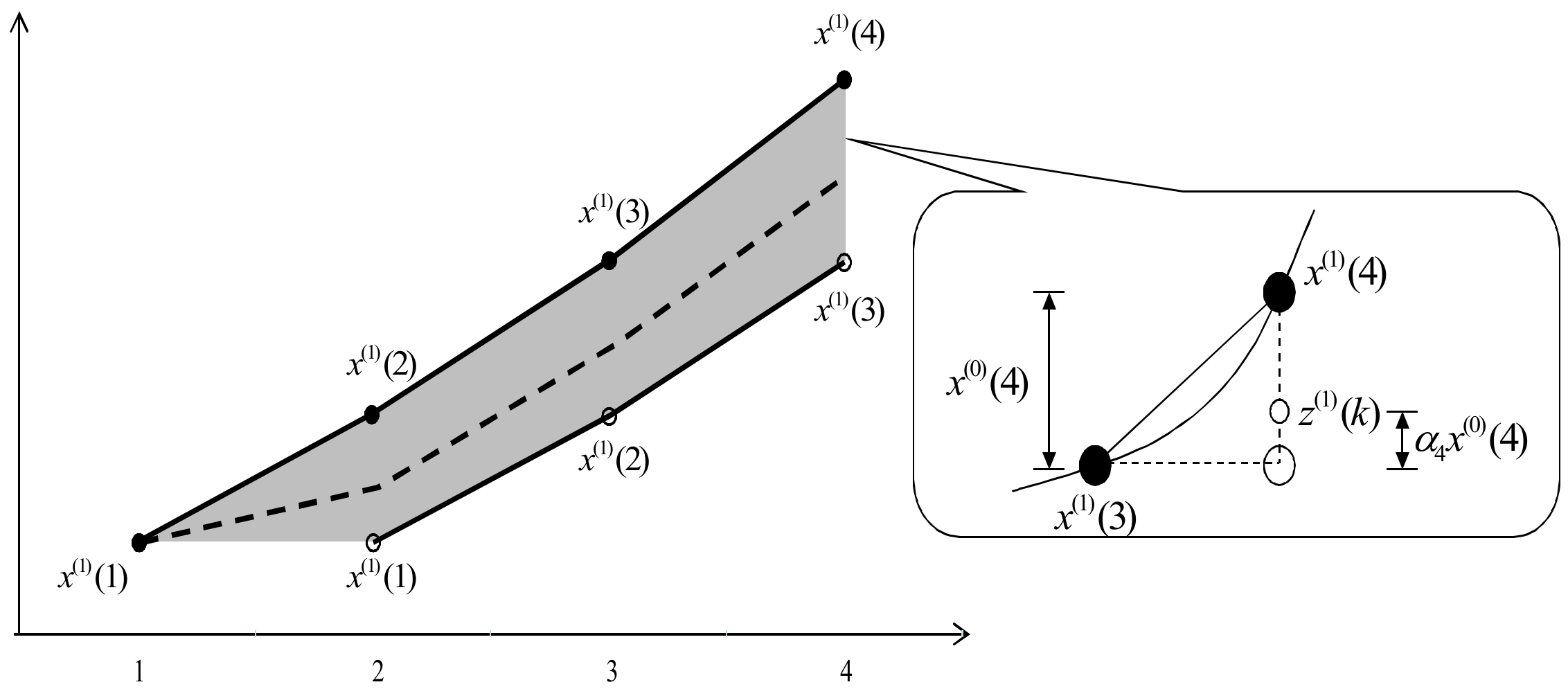
This research aims to improve the prediction accuracy of FGM (1,1) by determining the coefficient α sets, which affect the background values proposed by Wu et al. (2013) The core technique in this paper is to employ the new fractional order grey model based on boxplots and to find the coefficient α sets and will be named BP-FGM (1,1) hereafter. The most suitable background values would be located between ($x^{\left(1\right)}\left(k-1\right)$, $x^{\left(1\right)}\left(k\right)$), shown as the area colored in grey in Figure 2, where the dotted line represents the background values of the traditional GM model when α is set as a constant 0.5.

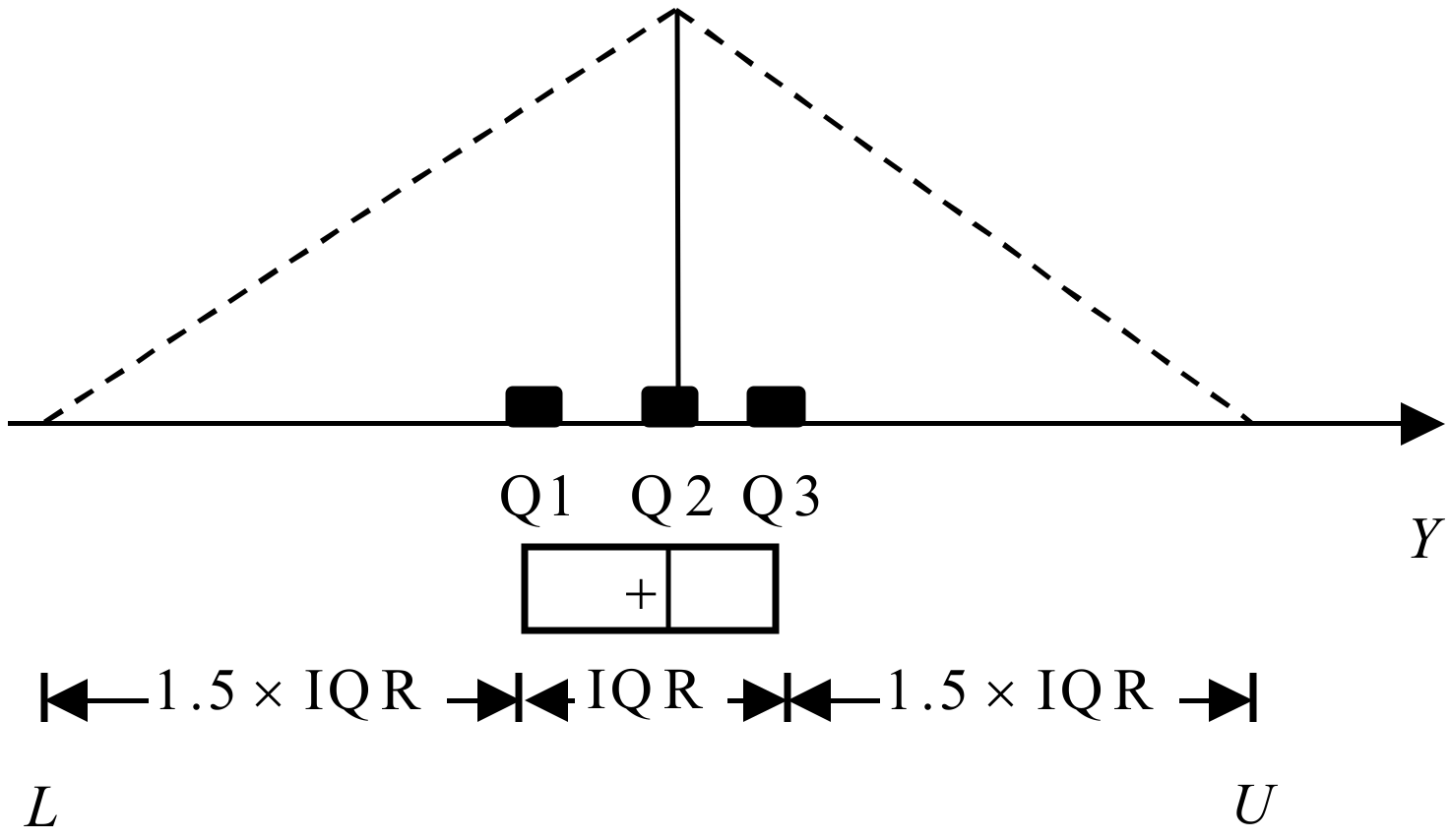
Firstly, it is necessary to build the shapes of attribute sample distributions and the triangular membership functions (MF), shown in Figure 3, by adopting the suitable ranges defined by the box-and-whisker plots (called boxplots hereafter).

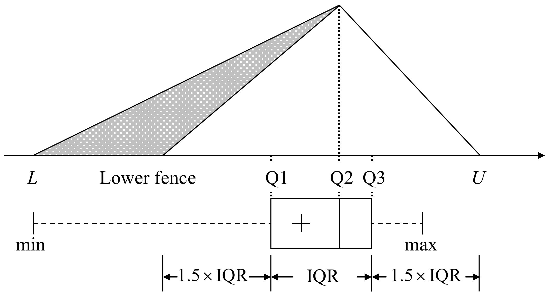
As in Section 2.1, boxplots contains three sections and each section contains its upper bound (Q1) and lower bound (Q3). The appropriate value bounds [L, U] defined in the boxplots and called the inner fences, where L is the lower fence, defined as $1.5\times \mathrm{IQR}$ lower than Q1 and U is the upper fence defined as $1.5\times \mathrm{IQR}$ higher than Q3. Observations distributed outside the bounds can be recognized as outliers, while those distributed within the bounds [L, U] are recognized as reasonable observations. However, it is easy to misclassify a reasonable observation as an outlier when sample sizes are small. The estimated bounds are thus modified as

$$\mathrm{L}=\left\{\begin{array}{c}\mathrm{Q}1-1.5\times \mathrm{I}\mathrm{Q}\mathrm{R} , \mathrm{L}\le min\\ min , \mathrm{L}>min\end{array}\right.$$

(5)

$$\mathrm{U}=\left\{\begin{array}{c}\mathrm{Q}3+1.5\times \mathrm{I}\mathrm{Q}\mathrm{R} , \mathrm{U}\ge max\\ max , \mathrm{U}<max\end{array}\right.$$

(6)

where min and max denote the minimum and maximum values of the observations, respectively, and are presented in Figure 4.

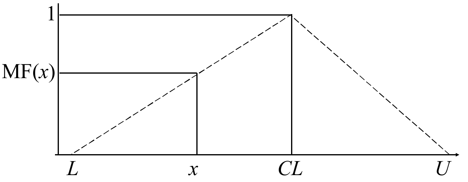
When the domain bounds of observations are obtained, the possible sample distribution can be demonstrated by drawing a triangular membership function (MF), using L, Q2, and U to represent it, as shown in Figure 5. The reason to take Q2 (or the median, Me) as the central location is that it is more sensitive than the average (or mean) when sample sizes are small. The MF is formulated as:

$$\mathrm{MF}\left(x\right)=\left\{\begin{array}{c}1 ,x=\mathrm{CL}\\ \frac{x-L}{\mathrm{CL}-L} ,x<\mathrm{CL}\\ \frac{U-x}{U-\mathrm{CL}} ,x>\mathrm{CL}\end{array}\right.$$

(7)

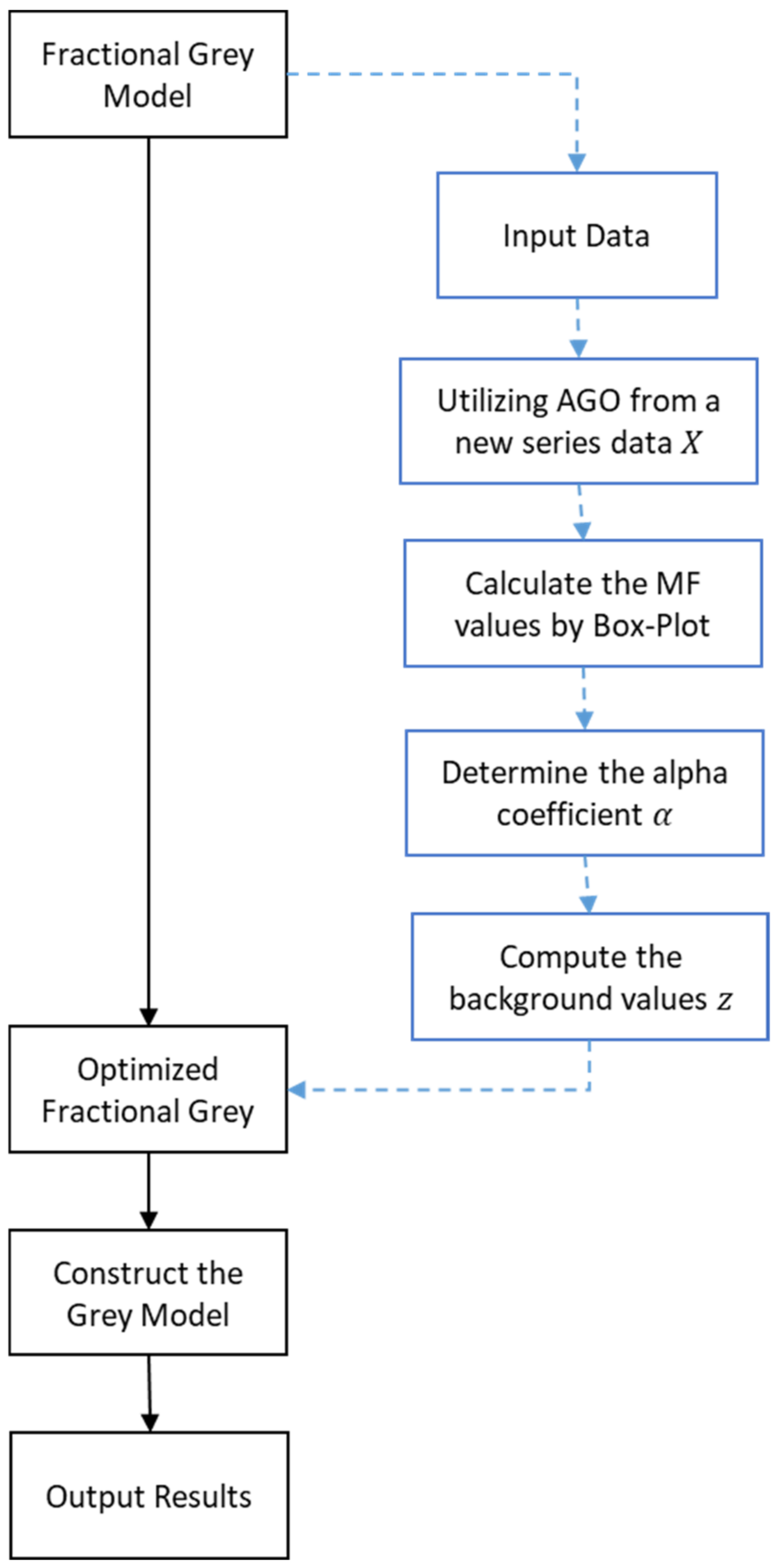
The procedure for building the BP-FGM (1,1) model are described in following steps, as shown in Figure 6. Let the original sequence be: $\left\{x^{\left(0\right)}\left(1\right),x^{\left(0\right)}\left(2\right),\dots ,x^{\left(0\right)}\left(n\right)\right\}$.

Step 1. Obtain coefficient α set by MF process, which is

$$\left\{MF\left(x^{\left(0\right)}\left(1\right)\right),MF(x^{\left(0\right)}\left(2\right)),\dots ,MF(x^{\left(0\right)}\left(n\right))\right\}$$

(8)

where $MF\left(x^{\left(0\right)}\left(1\right)\right)=1when i=1$.

Step 2. Generate a new sequence through the accumulating generation operator (AGO):

$$X^{\left(1\right)}=\left\{x^{\left(1\right)}\left(1\right),x^{\left(1\right)}\left(2\right),\dots ,x^{\left(1\right)}\left(n\right)\right\} ; x^{\left(1\right)}\left(1\right)=x^{\left(0\right)}\left(1\right)$$

(9)

$$x^{\left(r\right)}\left(\kappa \right)={\displaystyle \sum }_{i=1}^{\kappa }\frac{\mathsf{\Gamma }\left(r+k-i\right)}{\mathsf{\Gamma }\left(k-i+1\right)\mathsf{\Gamma }\left(r\right)}{x}^{\left(0\right)}\left(i\right), k=2,3,\dots ,n$$

(10)

Step 3. Calculate the background values, $z^{\left(r\right)}\left(\kappa \right)=\frac{1}{2}\left[x^{\left(r\right)}\left(k\right)+x^{\left(r\right)}\left(k-1\right)\right]$, which can be written as

$$z^{\left(1\right)}\left(\kappa \right)=\left(1-\alpha \right)x^{\left(1\right)}\left(k-1\right)+\alpha x^{\left(1\right)}\left(k\right), \alpha ϵ\left(0,1\right), k=2,3,\dots ,n$$

(11)

Step 4. Calculate the whitenization differential equation:

$$x^{\left(r\right)}\left(\kappa \right)-x^{\left(r\right)}\left(\kappa -1\right)+a{z}^{\left(r\right)}\left(\kappa \right)=b$$

(12)

$$\frac{d{x}^{\left(r\right)}\left(t\right)}{dt}+a{x}^{\left(r\right)}\left(t\right)=b$$

(13)

Step 5. Use the equation in Step 4 to estimate the developing coefficient a and the grey input b by the ordinary least-square method. Then establish the grey differential equation by employing Equation (12) to replace the source model.

Step 6. Solve Equation (12) with the initial condition $x^{\left(1\right)}\left(1\right)=x^{\left(0\right)}\left(1\right)$ and the desired forecasting output at the k+1 stage can be obtained through:

$${\widehat{x}}^{\left(r\right)}\left(\kappa +1\right)=\left(x^{\left(0\right)}\left(1\right)-\frac{b}{a}\right)e^{-ak}+\frac{b}{a}$$

where $\kappa =1,2,\dots ,n-1,\gamma \in R_{+},0<\gamma \le 1$.

4. Experimental Results and Discussion

In the experiment, real information containing sales data of specific customers taken from a leading company was used and the other dataset was obtained from the Department of Statistics of the Ministry of Economic Affairs (called MOEA hereafter), which is open data provided by government. This section will explain the result and adopt the index to measure the prediction accuracy.

4.1. Data from This Case Study

The production time-series prospects for the five months from August 2021 to December 2021 are shown in

Table 1. The dataset collected from Company A.

Month of 2021	Company A
August	39
September	37
October	42
November	40
December	41

.

4.2. MOEA Data

The production and sales data obtained from MOEA for the 12 months from January 2021 to December 2021 is shown in

Table 2. The dataset collected from MOEA, Company B and C.

Month of 2021	Company B	Company C
January	1072	1051
February	1011	1006
March	1262	1190
April	1051	1067
May	1121	1085
June	1151	1103
July	1111	1111
August	1162	1143
September	1212	1143
October	1191	1124
November	1234	1120
Dec	1279	1175

. The experiment dataset can be downloaded at https://dmz26.moea.gov.tw/GMWeb/investigate/InvestigateDA.aspx, accessed on 10 January 2022, the operation of this webpage is needed to include sales and manufacturers’ shipments, product category and time periods.

4.3. Analysis of the Experimental Results

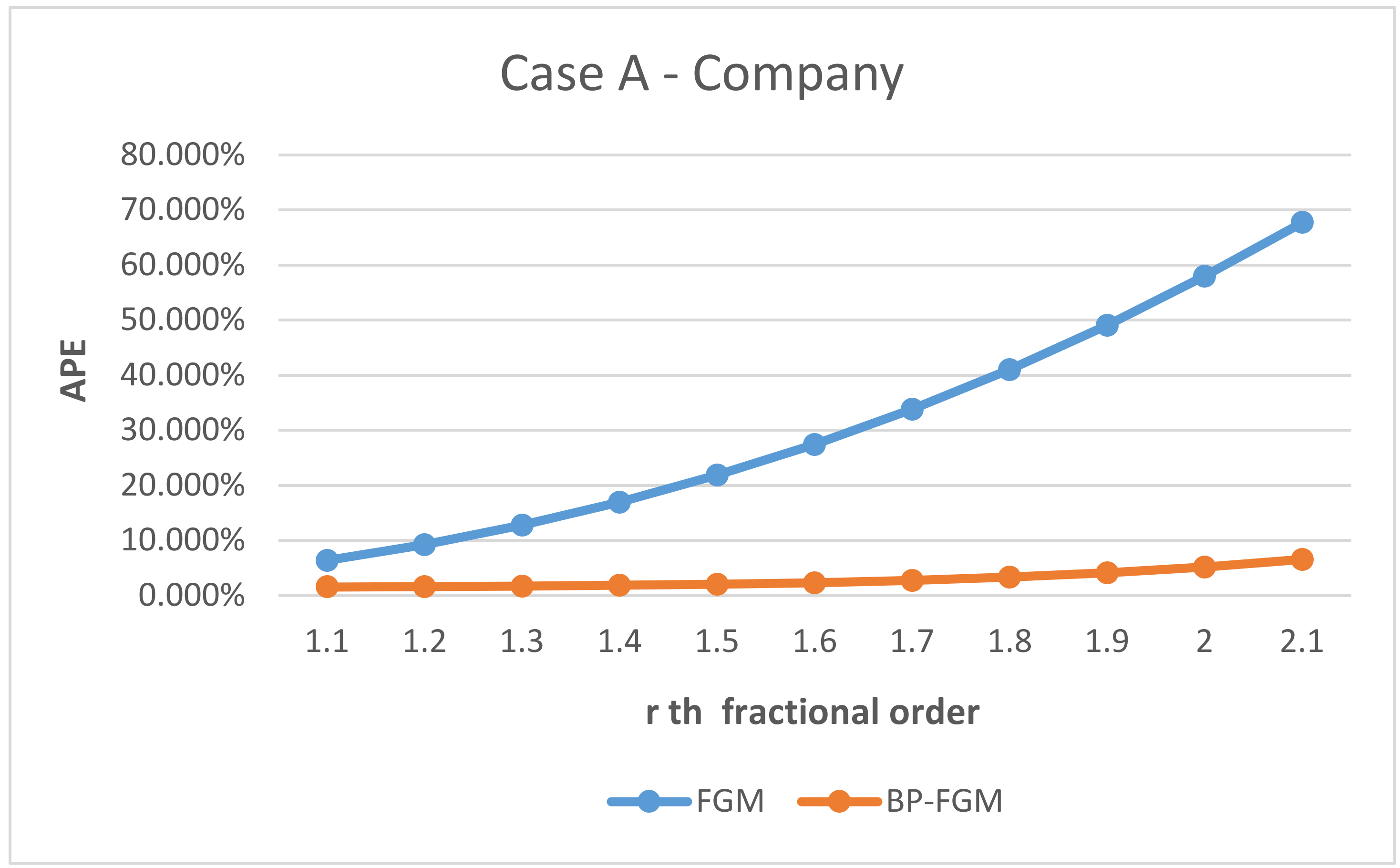
In addition, this study tried to identify whether there was a significant difference in the prediction errors between the FGM (1,1) and BP-FGM (1,1) models. Three datasets were used and 11th fractional orders were performed in the experiment. Additionally, the absolute percentage error (APE) is used as the error index for each order. The formula is shown in (14). After calculating the prediction errors of all the data, we were able to use the MAPE as the error measurement, as shown in (15).

$$APE=\left|\frac{y_i-{\widehat{y}}_i}{y_i}\right|\times 100\%$$

(14)

$$MAPE=\left|\frac{1}{N-4}\right|{\displaystyle \sum }_{i=5}^{N}AP{E}_i$$

(15)

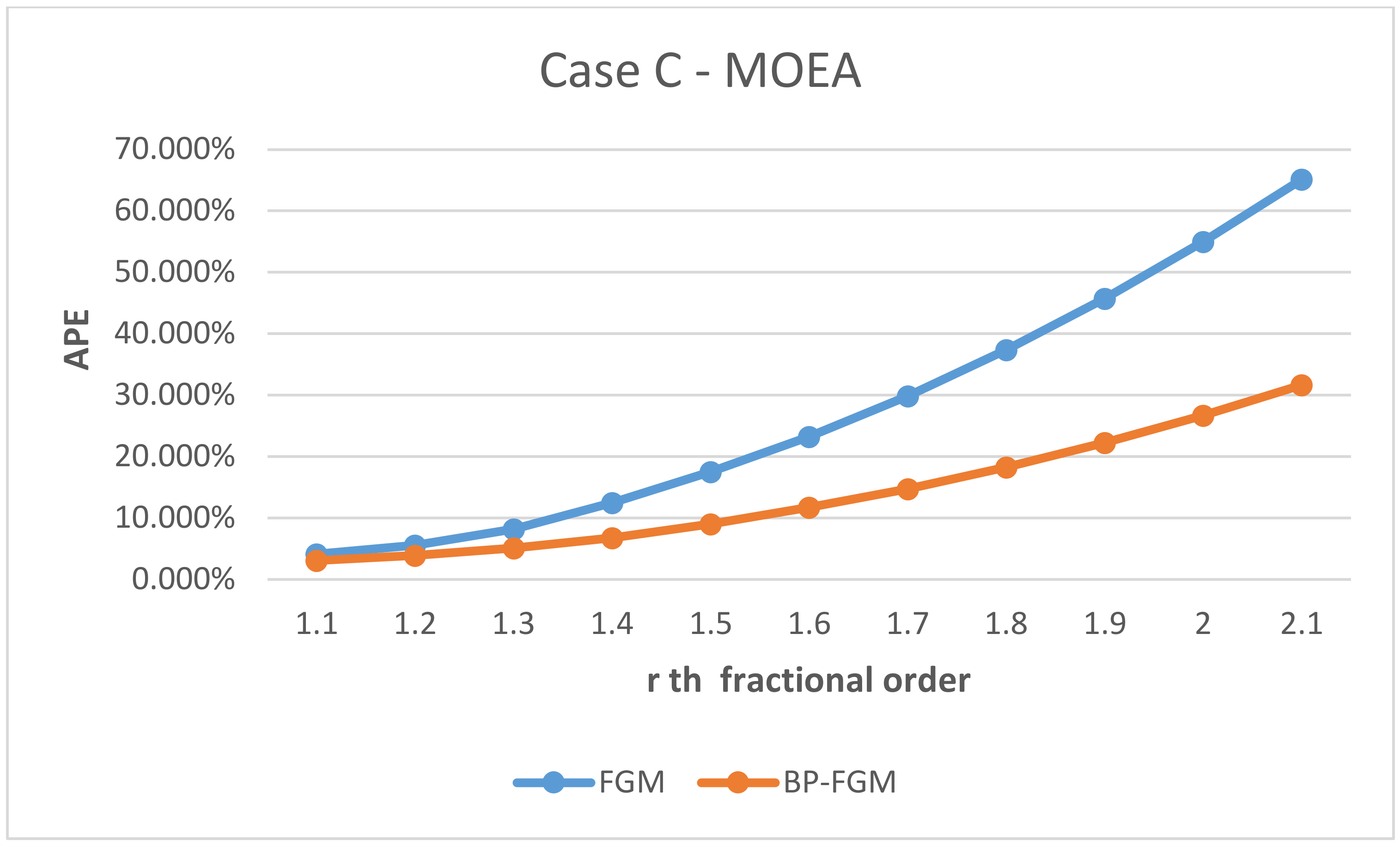
The experiment results from the data of the company and MOEA are summarized in

Table 3. The summary of experiment errors by using the FGM and BP-FGM models.

Case/MAPE (%)	FGM (1,1)	BP-FGM (1,1)
Company A	31.303%	17.152%
Company B	27.062%	19.195%
Company C	27.641%	20.775%

, where the errors are MAPEs (mean absolute percentage error) calculated by Equation (15). The detailed results are shown in Figure 7, Figure 8 and Figure 9, where the errors are APEs (absolute percentage error) commutated by Equation (14) for 11 fractional orders that start from 1.1 to 2.1. The lower the APE values, the higher the indication of prediction accuracy.

5. Conclusions

Computers, communications and consumer products go hand in hand with our life. Suppliers of various brands need to continuously carry out new product research and development. If the demand can be accurately predicted, it will be of great help to enterprise decision makers and production equipment suppliers.

To forecast the production and demand of downstream customers, this research reveals a new grey model which uses boxplots to estimate the trend of data and, if this is combined with FGM, it is known as the boxplot-based fractional scale prediction model (boxplot-based FGM, BP-FGM), which improves the accuracy of predictors by setting the coefficient sets of α in traditional grey model, even if there is no large amount of past data [17,18].

In the experiment, we try to observe the demand pattern of customers through the new grey prediction model BP-FGM (1,1). The difference between FGM (1,1) and BP-FGM (1,1) is that the improvement of FGM (1,1) aims to explore the suitable background value to make the prediction value more accurate. BP-FGM (1,1) not only uses the advantages of the fractional cumulative grey prediction model, FGM (1,1), but adopts the concept of the fuzzy sequence set that introduced box-and-whisker plots combined with triangular membership functions to estimate the trend of data in order to fuzzify the time-series data, and then, through the GM modeling procedure, improves the prediction accuracy, as is illustrate in Figure 6.

For modeling, MAPE is established to be acting as the objective function of the optimization model, the results from the three datasets verified the effect through the commodity attributes and public test data of its production, and the experimental results show that BP-FGM has better prediction results than FGM.

In this study, we focused on the new product demand of the semiconductor industry only, experiments for different research, such as weather and temperature forecasts, grain yield or short-term electricity demand, may be studied in future work.

References

- Mas-Machuca, M.; Sainz, M.; Martinez-Costa, C. A review of forecasting models for new products. Intang. Cap. 2014, 10, 1–25. [Google Scholar] [CrossRef] [Green Version]
- Li, D.-C.; Chen, W.-C.; Chang, C.-J.; Chen, C.-C.; Wen, I.-H. Practical information diffusion techniques to accelerate new product pilot runs. Int. J. Prod. Res. 2015, 53, 5310–5319. [Google Scholar] [CrossRef]
- Chien, C.-F.; Chen, Y.-J.; Peng, J.-T. Manufacturing intelligence for semiconductor demand forecast based on technology diffusion and product life cycle. Int. J. Prod. Econ. 2010, 128, 496–509. [Google Scholar] [CrossRef]
- Deng, J.L. Control problems of grey systems. SCL Syst. Control Lett. 1982, 1, 288–294. [Google Scholar]
- Mao, S.; Gao, M.; Xiao, X.; Zhu, M. A novel fractional grey system model and its application. Appl. Math. Model. 2016, 40, 5063–5076. [Google Scholar] [CrossRef]
- Deng, J.L. Introduction to Grey system theory. J. Grey Syst. 1989, 1, 1–24. [Google Scholar]
- Wu, L.; Liu, S.; Fang, Z.; Xu, H. Properties of the GM(1,1) with fractional order accumulation. Appl. Math. Comput. 2015, 252, 287–293. [Google Scholar] [CrossRef]
- Wu, L.; Liu, S.; Yao, L.; Yan, S.; Liu, D. Grey system model with the fractional order accumulation. Commun. Nonlinear Sci. Numer. Simul. 2013, 18, 1775–1785. [Google Scholar] [CrossRef]
- Xie, W.; Wu, W.-Z.; Liu, C.; Goh, M. Generalized fractional grey system models: The memory effects perspective. ISA Trans. 2021. [Google Scholar] [CrossRef] [PubMed]
- Yuxiao, K.; Shuhua, M.; Yonghong, Z. Variable order fractional grey model and its application. Appl. Math. Model. 2021, 97, 619–635. [Google Scholar] [CrossRef]
- Hu, Y.-C.; Jiang, P.; Tsai, J.-F.; Yu, C.-Y. An Optimized Fractional Grey Prediction Model for Carbon Dioxide Emissions Forecasting. Int. J. Environ. Res. Public Health 2021, 18, 587. [Google Scholar] [CrossRef] [PubMed]
- Huang, H.; Tao, Z.; Liu, J.; Cheng, J.; Chen, H. Exploiting fractional accumulation and background value optimization in multivariate interval grey prediction model and its application. Eng. Appl. Artif. Intell. 2021, 104, 104360. [Google Scholar] [CrossRef]
- Zhao, L.; Zhou, X. Forecasting Electricity Demand Using a New Grey Prediction Model with Smoothness Operator. Symmetry 2018, 10, 693. [Google Scholar] [CrossRef] [Green Version]
- Li, D.-C.; Chang, C.-J.; Chen, C.-C.; Chen, W.-C. Forecasting short-term electricity consumption using the adaptive grey-based approach—An Asian case. Omega 2012, 40, 767–773. [Google Scholar] [CrossRef]
- Tukey, J.W. Exploratory Data Analysis; Reading, Mass.; Addison-Wesley: Menlo Park, CA, USA; London, UK; Amsterdam, The Netherlands, 1977. [Google Scholar]
- Salkind, N.J. Encyclopedia of Research Design; SAGE: Newbury Park, CA, USA, 2010. [Google Scholar] [CrossRef]
- Shah, I.; Bibi, H.; Ali, S.; Wang, L.; Yue, Z. Forecasting One-Day-Ahead Electricity Prices for Italian Electricity Market Using Parametric and Nonparametric Approaches. IEEE Access 2020, 8, 123104–123113. [Google Scholar] [CrossRef]
- Shah, I.; Akbar, S.; Saba, T.; Ali, S.; Rehman, A. Short-Term Forecasting for the Electricity Spot Prices with Extreme Values Treatment. IEEE Access 2021, 9, 105451–105462. [Google Scholar] [CrossRef]
Figure 1.
Illustration of a box plot.
Figure 2.
The possible area indicating where background values would be located.
Figure 3.
The reasonable ranges can be defined by the box-and-whisker plots.
Figure 4.
Using triangular MFs to form the shape of the attribute distribution.
Figure 5.
Representing the membership function.
Figure 6.
Flowchart of the BP-FGM (1,1).
Figure 7.
Representing the absolute percentage error for Case A by using the FGM and BP-FGM model.
Figure 8.
Representing the absolute percentage error for Case B by using the FGM and BP-FGM model.
Figure 9.
Representing the absolute percentage error for Case C by using the FGM and BP-FGM model.