Analysis and Modeling of Mechanical Ventilation Operation Behaviors of Occupants in Cold Regions of North China

Abstract

Mechanical ventilation has a great impact on building simulation performance, such as indoor environment quality and building energy consumption. However, there is still a lack of accurate mechanical ventilation models established from long-term field data that can effectively predict building performance. In this study, one-year measurements on mechanical ventilation operation behavior were collected from 85 apartments, which were conducted with a mechanical ventilation system of the same brand in cold regions of North China. This permitted statistical analysis and clustering of the mechanical ventilation operation behavior by using the K-means method, leading to five behavior patterns. The results showed that 24% households operated mechanical ventilation system nearly all day, and there was a large difference in usage behaviors between the split system and the centralized system. Furthermore, two classes of models based on random forest and logistic regression were developed for predicting mechanical ventilation system operation (on/off) behavior. The models based on random forest showed high accuracy as it resulted in a 0.992 average in predictions. These models using field data can guide the selection of accurate input boundary conditions of mechanical ventilation and improve the accuracy of dwelling numerical simulations.

1. Introduction

Modern people spend 80–90% of their time indoors [1,2], and most diseases related to environmental exposures stem from indoor air exposure [3]. For example, exposure to high PM_2.5 concentrations can cause chronic respiratory symptoms [4], even lung cancer [5], while other air pollutants scuh as the ozone can affect cardiovascular health [6,7,8]. Ventilation is effective in diluting or removing indoor air pollutants, for which the methods can be categorized into two main types, i.e., natural and mechanical. Mechanical ventilation is more effective and reliable than natural ventilation for improving indoor air quality and comfort. People have started to pay increasing attention to the improvement of indoor environment in recent years, making mechanical ventilation systems become popular in newly built or renovated apartments. To develop reasonable ventilation strategies in residential buildings, it is necessary to study mechanical ventilation system operation behaviors of residents.

Previous studies on mechanical ventilation system operation behavior mainly focused on behavior patterns, the impact on indoor environment and energy consumption. Lai et al. [9] conducted an investigation on the usage of mechanical ventilation in 46 dwellings in different cities in China, finding that the daily mechanical ventilation duration was 7.2 h on average and there were large differences in ventilation duration among climate regions and seasons. Zhao and Liu [10] conducted a measurement study on 36 apartments and found that the duration of mechanical ventilation systems operation increased as outdoor PM_2.5 concentrations increased. Zhao [11] analyzed the indoor climate of nine households and found that operating mechanical ventilation system in winter in Urumqi, China, reduced indoor temperatures by 1.6 K and humidity by 3% on average, and residents were more likely to sense dryness. Mechanical ventilation systems were also found to have positive effects on the different pollutants (e.g., CO₂, sub-micron particles and PM₁₀) [12,13,14], but the relevant cost can be more than twice of that for natural ventilation [15]. Park et al. [16] conducted a survey of 139 residential apartments in Seoul, Korea, and found that about 68.3% of the occupants did not use mechanical ventilation fans during the heating period because of the increasing costs in heating energy. Kim et al. [17] found that CO₂ concentrations were the most influential driver for occupant ventilation behavior.

To design automatic, efficient and energy-saving ventilation, building simulation performance is widely used [18], for which the operation behavior of the mechanical ventilation system is one of the important input items. However, most existing studies used the fixed schedule and ventilation volume to describe the operation state of mechanical ventilation system. Some studies used idealized feedback set mode, in which the system will switch on when indoor CO₂ and PM_2.5 concentrations are over the preset thresholds [15,19], or economizing strategy, for which the supply airflow of mechanical ventilation system is automatically sized when the outdoor air temperature is low enough to provide free-cooling effectively [20]. In general, these methods cannot well represent the complex and changeable occupant mechanical ventilation behavior in reality, which can result in large discrepancies between the predicted results and the measured data [18,21]. To improve the accuracy in dynamic building performance simulation, there is a need to develop accurate mechanical ventilation models with field data.

Currently, with the development of IoT (Internet of Things) and big data, by combining computer science, statistics and database knowledge, machine learning techniques have been widely used to develop occupant behavior predictive model with improved performance. Ren et al. [22] used clustering analysis to identify the motivation patterns of the mechanical ventilation flowrate adjustment behaviors from 10 dwellings. Liu et al. [23] found that the air conditioner’s operation behavior models developed by ANN and GBDT algorithms showed higher accuracy than logistic regression. Cho et al. [24] applied Generalized Additive Models to analyze occupants’ window-opening behavior. Using occupant data from commercial buildings in Germany, Markovic et al. [25] proposed a window opening model with deep learning methods, and the evaluation accuracy was between 86 and 89%. Mo et al. [26] studied the prediction model of occupant window behavior in residential buildings and concluded that the XGBoost algorithm showed better performance with high accuracies of around 80%. However, studies on mechanical ventilation operation behavior are limited.

In order to narrow the deviation between simulation results and reality, in this study, the actual environment parameters and mechanical ventilation behavior data of residents were collected from 85 houses in Hebei province and Beijing and Tianjin in China. Moreover, the behavior patterns of two types of ventilation systems (i.e., split and centralized) were investigated by statistical analysis. Moreover, logistic regression and random forest models were built using the collected data, and their predictive performance were evaluated.

2. Methods and Data

2.1. Monitored Households and Mechanical Ventilation System

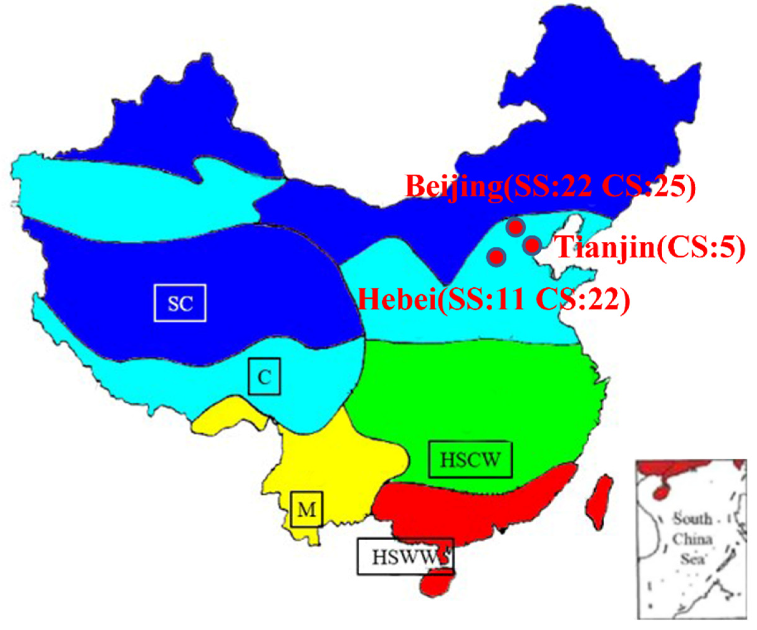
The climate zone distributions of China [23] and the location and quantity distribution of the monitored households are shown in Figure 1. These households were in the cold region of northern China. They were in Beijing, Tianjin and six cities of Hebei province (Shijiazhuang, Baoding, Langfang, Cangzhou, Tangshan and Handan). All these households were using a mechanical ventilation system of the same brand. There were two types of systems, either split or centralized, with schematics provided in Figure 2 and relevant parameters listed in

Table 1. Parameters of mechanical ventilation system.

Parameter	Split	Centralized
Air flow (m3/h)	60–130	100–500
Usage area (m2)	30	120–180
Rated power (W)	22	165
Noise (dB)	32–49	29–56
Product size (mm)	840 × 300 × 185	1541 × 600 × 405
Net weight (kg)	13.8	65

.

The split system is a supply ventilation system with one air inlet [9]. Each room uses it independently. In this study, most split systems were installed in bedrooms. It uses a fan to force outdoor fresh air into the room through the filter element, while the indoor exhausted air leaks out through the cracks and holes of the building. The centralized system is an energy recovery ventilation system with ducts. It can generally be used in the entire house. The fresh air is introduced and sent to each room through the air inlet duct, and the exhausted air is discharged outdoors through the exhaust duct. Meanwhile, the operation of the heat exchange unit makes the occupant feel more thermally comfortable and saves heating loads in the winter season and cooling loads in the summer season.

2.2. Long-Term Field Data Collection and Preprocessing

The data in this research were collected from 1 January 2018 to 31 December 2018. A sensor module applied to the mechanical ventilation system was used to monitor indoor environmental parameters including temperature, CO₂ and PM_2.5 concentration. In addition, the system’s status (i.e., power on/off) and air flow were collected in every 5 min. Outdoor environmental parameters including temperature, relative humidity and PM_2.5 concentrations were obtained from the weather stations near the monitored households at a time interval of 2 h. The timestamp interval of outdoor environmental data was preprocessed as 5 min by forward filling, which is consistent with indoor environmental data. Missing values, outliers and inconsistencies were removed and forward filled.

2.3. Model

2.3.1. K-Means

Clustering not only can be used as a separate process to find the internal structure and regularity of data but also can be used as a precursor process for supervised learning tasks such as classification. K-means algorithm is one of the widely utilized clustering algorithm [27]. In this study, the K-means algorithm was used to for clustering and analyzing the similarities and differences of the mechanical ventilation operation behavior of occupants.

Given a sample set X = {x₁, x₂, …, x_n}, the K-means algorithm divides X into K clusters C. Each cluster has its “centroid” μ_j (j = 1, 2, …, K) obtained by averaging the samples in this cluster. The K-means algorithm aims to select the optimal cluster partition by minimizing the squared error.

$${\sum }_{i=0}^{n}min\left(\Vert x_i-{\mu }_j\Vert {}^2\right)$$

(1)

The algorithm is composed of three steps. Firstly, k centroids are initialized, where a naive method is to randomly choose k samples from X. Secondly, each sample in X is assigned to its nearest centroid. Thirdly, the mean value of the samples for each cluster as the new centroid is recalculated. The differences between the old and the new centroids are computed, and the algorithm repeats the last two steps unless the difference is less than a threshold.

The Silhouette Coefficient is usually used to evaluate the performance of a cluster analysis without knowing the true cluster label [28]. A higher Silhouette Coefficient score indicates a model with better defined clusters:

$$S=\frac{{\sum }_{i=1}^n\frac{b\left(i\right)-a\left(i\right)}{max\left\{a\left(i\right),b\left(i\right)\right\}}}{n}$$

(2)

where S is the Silhouette Coefficient score, a(i) is the average distance between sample i and all other samples within the same cluster and b(i) is the minimum average distance between i and all samples in any other clusters.

2.3.2. Logistic Regression

In this study, sets 0 and 1 denote the off and on states of the mechanical ventilation system’s status, respectively. Thus, the prediction model can be a binary classification problem. Logistic regression algorithm is a classic classification algorithm [29] and has been widely used in modeling occupant behavior [22,23,25,30]. It can be represented by the probability function, as described by Equation (3):

$$logit p=log\left(\frac{p}{1-p}\right)=b+c_1{x}_1+c_2{x}_2+\dots +c_n{x}_n$$

(3)

where p is the probability of the mechanical ventilation system turning on/off event, b is the intercept, $c_1$, $c_2$, …, $c_n$ are the coefficients of variables and $x_1$, $x_2$, …, $x_n$ are the explanatory variables (i.e., indoor and outdoor environmental parameters and time parameters).

2.3.3. Random Forest

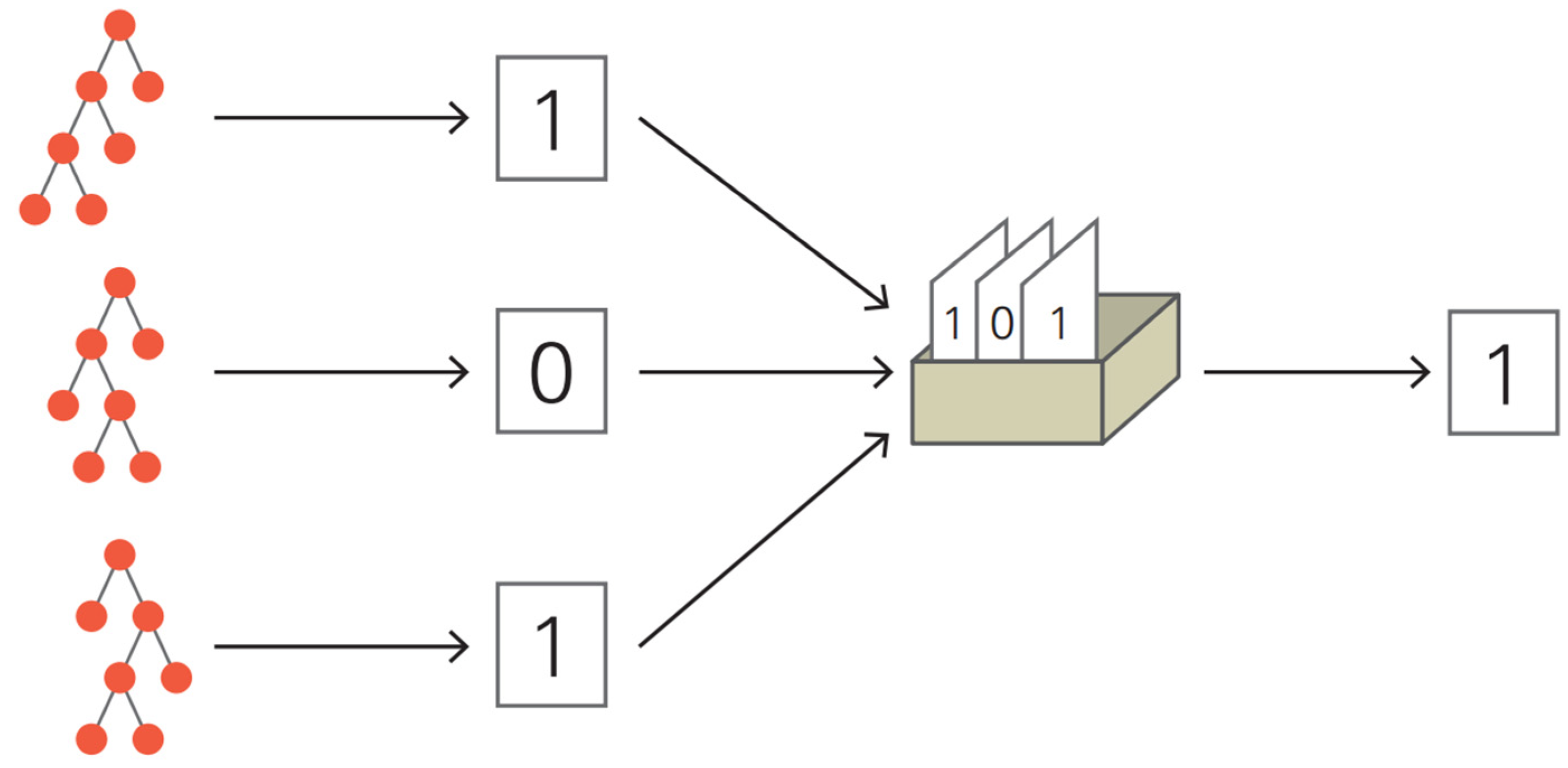
Random forest is a classification algorithm combining multiple decision tree models to obtain higher prediction accuracy (than a single decision tree), and it possesses stronger generalization ability [31]. The schematic of random forest is shown in Figure 3.

In random forests, each tree in the ensemble is built from a sample drawn with replacement (i.e., a bootstrap sample) from the training set. Furthermore, when splitting each node during the construction of a tree, the best split is found either from all or a random subset of the input features. Using two methods, i.e., “Bootstrap method” and “Random selection of eigenvalues”, a decision tree with diversity can be trained.

2.4. Model Evaluation Criteria

Classification accuracy (ACC) is the commonly used indicator for evaluating the performance of classifiers. For a given test dataset, ACC is the ratio of the number of correctly classified samples to the total number of samples, defined by Equation 4. It is based on a matrix of actual data and predicted data, called confusion matrix, as shown in

Table 2. Confusion matrix.

Actual Data	Prediction
	0	1
0	TP	FN
1	FP	TN

TN: true negative; FP: false positive; FN: false negative; TP: true positive.

.

$$\mathrm{ACC}=\frac{\mathrm{TP}+\mathrm{TN}}{\mathrm{TP}+\mathrm{FP}+\mathrm{TN}+\mathrm{FN}}$$

(4)

However, when the imbalance of data is high, which means the number of positive data and the number of negative data have a large deviation, the ACC indicator does not work well [32]. Moreover, the area under the curve (AUC) indicator can deal with the problem of dataset imbalance [33].

AUC refers to the area under the receiver operating characteristic (ROC) curve. The horizontal axis of the ROC curve is false positive rate (FPR), and the vertical axis is the true positive rate (TPR). The value of the area (i.e., AUC) is between 0 and 1. The closer the value of AUC is to 1, the better the performance of the model is.

$$\mathrm{TPR}=\frac{\mathrm{TP}}{\mathrm{TP}+\mathrm{FN}}$$

(5)

$$\mathrm{FPR}=\frac{\mathrm{TN}}{\mathrm{FP}+\mathrm{FN}}$$

(6)

3. Result and Discussion

3.1. Statistics of Behavior in Mechanical Ventilation Operation

3.1.1. Operation Duration of the Mechanical Ventilation System

An $r$ value is defined below to describe the operation duration of the mechanical ventilation system:

$$r=\frac{T_O}{T_a}\times 100\%$$

(7)

where $T_O$ and $T_a$ are the operating time of the system and the total time in a certain period, respectively.

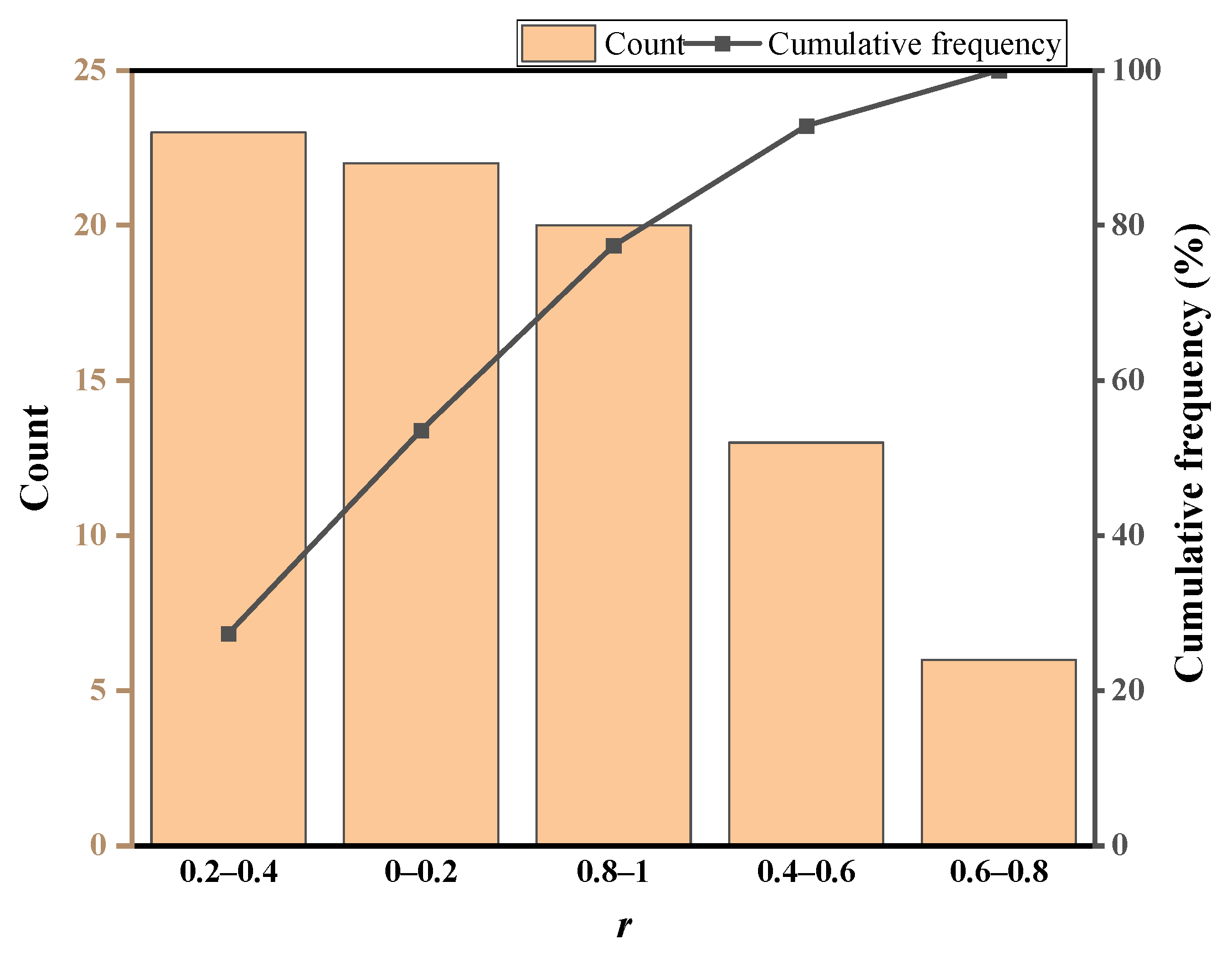
Figure 4 shows the Pareto chart of $r$ of all monitored households. It is clear that $r$ is mainly distributed between 0–0.2, 0.2–0.4 and 0.8–1. With 0.8 as the limit, the households are divided into two categories: system being on nearly all-day and system being on intermittently. There are 20 (24%) households in the former, and the average operating time is more than 20 h per day, while the average operating time of the latter households is 7 h per day. This suggests that the mechanical ventilation system operating-behavior varies greatly among these households. In the following, an analysis is conducted for the households that operated systems intermittently.

3.1.2. Operation Behavior in the Split and Centralized Mechanical Ventilation Systems

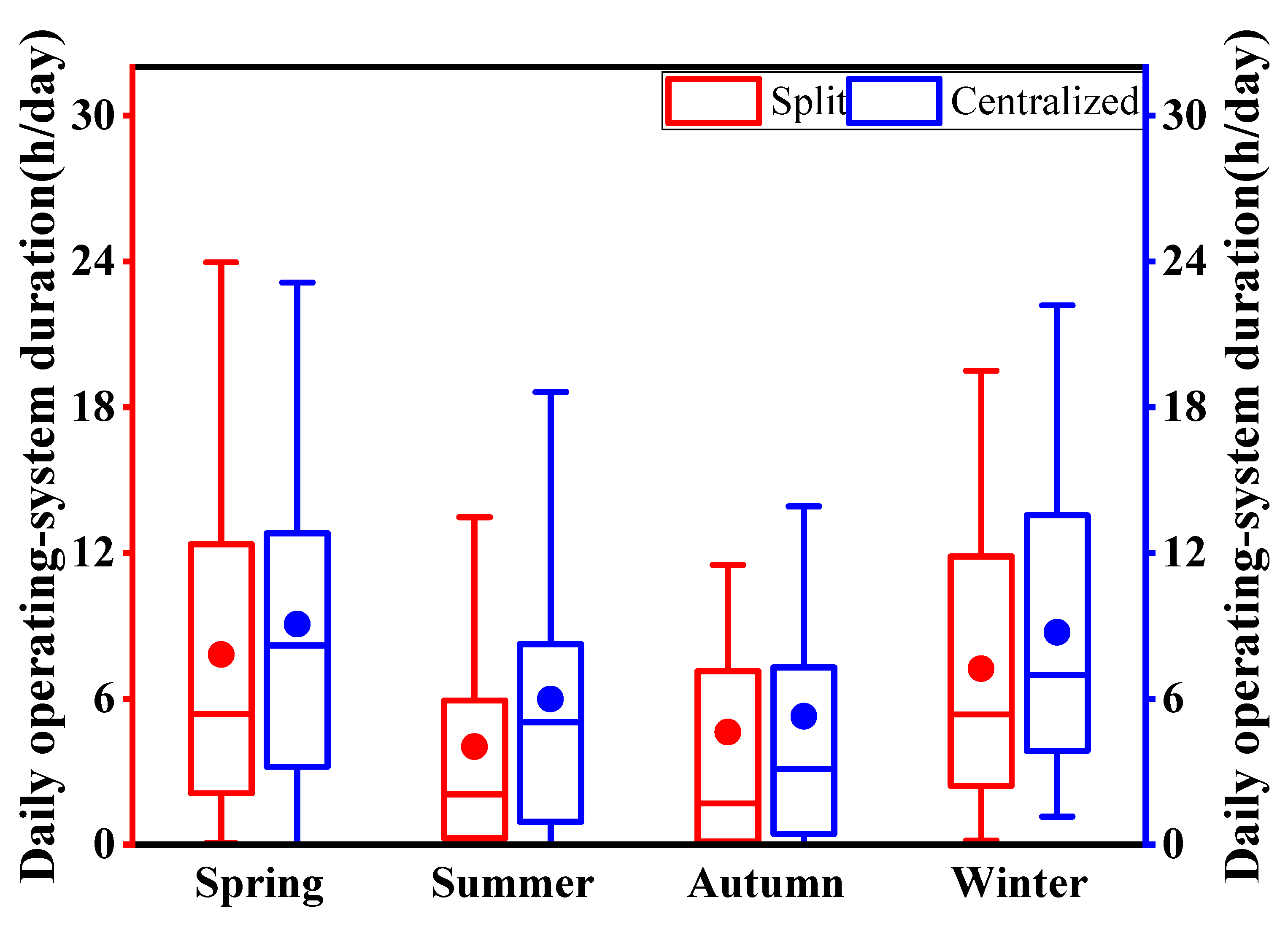
Figure 5 shows the boxplot of the average daily operation duration of the two mechanical ventilation systems in different seasons. Similar patterns could be observed between the two systems across four seasons, i.e., both of them had the longest operating-time in spring, followed by winter, and the shortest in summer and autumn. This is not consistent with what has been reported in Zhao’s study [10], probably due to differences of sample size, region, system brand and system type, etc. In addition, the average daily operation duration of the centralized system was longer than that of the split system in each season, which showed a difference of 1.3 h/day on average. Meanwhile, as shown in Figure 6, the operation of the split system over a year was more frequent than that of the centralized system, with an average operation of 192 and 145, respectively. According to these results, it can be seen that the split system was operated more frequently and flexibly, usually for a shorter duration, while the centralized system is responsible for supplying fresh air for the entire house, covering a larger area, and residents were more inclined to keep it operating for a longer period of time to maintain air quality in activity areas.

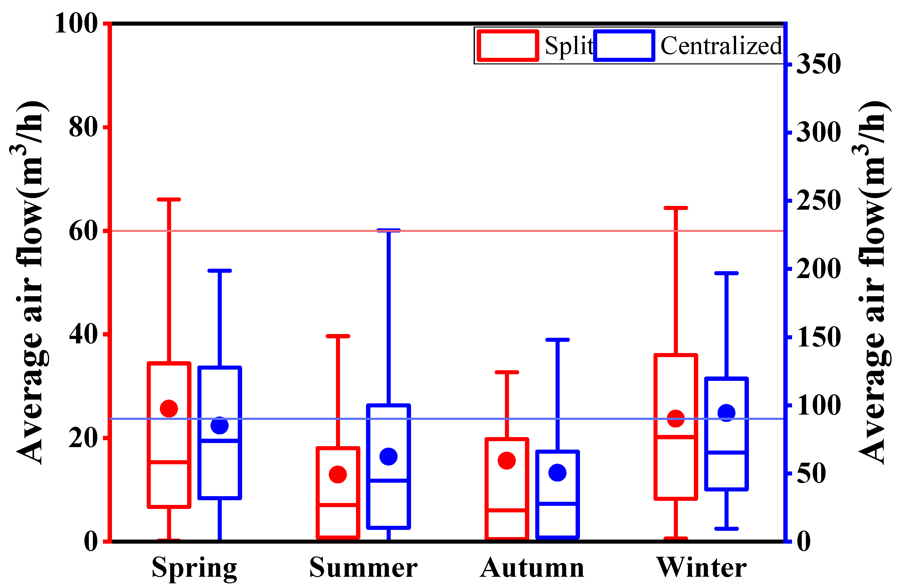
3.1.3. Operation Ventilation Flow Rate of Split and Centralized Mechanical Ventilation Systems

Figure 7 shows the boxplots of the ventilation flow rates of the two types of systems in different seasons. For the split system, the highest average ventilation volume was observed in spring, at 25.7 m³/h, while the lowest was observed in summer, at 13 m³/h. For the centralized system, the highest was observed in winter, at 94.4 m³/h, while the lowest was observed in autumn, at 50.4 m³/h. According to the Indoor Air Quality Standard (GB/T 18883-2002), the fresh air volume of residential buildings should not be less than 30 m³/h per person. Thus, the minimum fresh air volume of households with the split system should be 60 m³/h for two individuals, and the centralized system is 90 m³/h for three individuals. Since there are no window opening data in this study, without considering natural ventilation, it seemed that only the average mechanical ventilation volume of most households could not meet the fresh air need of human health. Relatively, the actual ventilation volume per person of households with the centralized system was better.

In addition, it was found that the variation of the mechanical ventilation volume of the centralized system in summer was larger than in other seasons, indicating that there were obvious differences (with p-value being 0.018 less than 0.05) in the usage behavior among different households in summer. Some households chose not to run the system or kept lower ventilation volumes probably because the air conditioner was turned on in summer, and the introduction of outdoor air through mechanical ventilation system would increase indoor temperatures and lead to a waste of energy. However, some occupants were willing to spend money on energy when the health requirement could be met by mechanical ventilation [9].

3.1.4. The Long-Term IAQ of Households with Mechanical Ventilation Systems

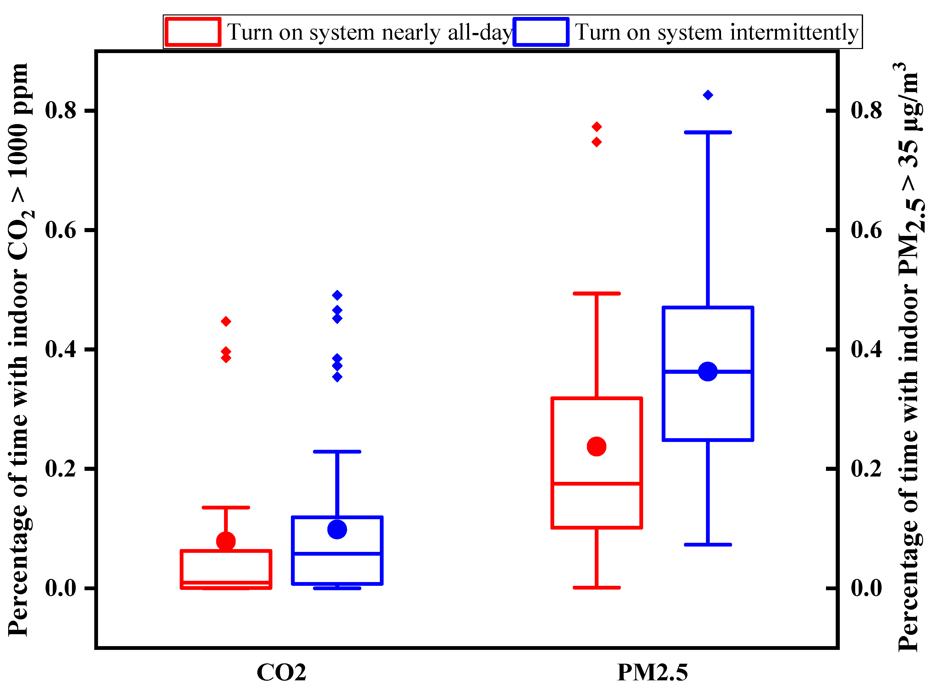
Figure 8 shows the boxplots of the percentage of time that the hourly average indoor CO₂ concentration exceeded 1000 ppm and when the indoor PM_2.5 concentration exceeded 35 μg/m³. Not considering outliers, for households that run the system nearly all day, the hourly average CO₂ concentration is above 1000 ppm for 0–14% of a year, and for households that run the system intermittently, it is 0–23%. Regarding indoor PM_2.5, correspondingly, the percentages of a year with concentration exceeding 35 μg/m³ is 0–49% in the former households and 7–76% in the latter households. Overall, the indoor air quality of the households using the system almost all day was better than that of intermittent use. However, different from the simulation results [15], even with the system operating throughout the day, IAQ cannot be good (with CO₂ concentration below 1000 ppm and PM_2.5 concentration below 35 μg/m³) at any time in reality.

In addition, several outliers on the boxplot are observed. For example, the proportion of indoor CO₂ concentration exceeding the standard is greater than 0.4, and the indoor PM_2.5 concentration exceeding the standard proportion is close to 0.8. This may be because the system has been running for a long time without cleaning and maintenance, and the dust of the filter element has accumulated substantially, increasing wind resistance, resulting in a reduction in the actual air supply volume, and secondary pollution will also occur, which affects purification effects. Therefore, it is necessary to replace the filter regularly for the households who often use the mechanical ventilation system.

3.2. Modeling of Behavior in Mechanical Ventilation Operation

The variables in this study include indoor CO₂ concentration (CO₂_In), indoor PM_2.5 concentration (PM_2.5_In), indoor temperature (T_In), outdoor PM_2.5 concentration (PM_2.5_Out), outdoor temperature (T_Out), outdoor relative humidity (RH_Out), hour (H), month (M) and the seasons (spring, summer, autumn and winter) that may have an impact on the system usage behavior. Moreover, the descriptive statistics information relative to them are shown in

Table 3. The descriptive statistics information of some variables.

	CO2_In	PM2.5_In	T_In	PM2.5_Out	T_Out	RH_Out
mean	678.46	53.45	24.69	56.92	13.52	49.58
std	398.55	157.47	3.77	55.08	12.50	24.13
min	400.00	0.00	5.00	0.00	−20.20	0.00
50%	646.00	20.00	25.00	41.00	14.80	48.00
max	5000.00	1000.00	38.00	500.00	41.5	100.00

.

3.2.1. K-Means Clustering

As observed from the previous analysis, there were differences in the behavior of operating mechanical ventilation systems among different households, where it requires multiple models to cover all cases. In this regard, K-means cluster analysis would be helpful. Moreover, the Pearson correlation coefficients between the status of the mechanical ventilation system and external factors were used as the input feature of the cluster analysis.

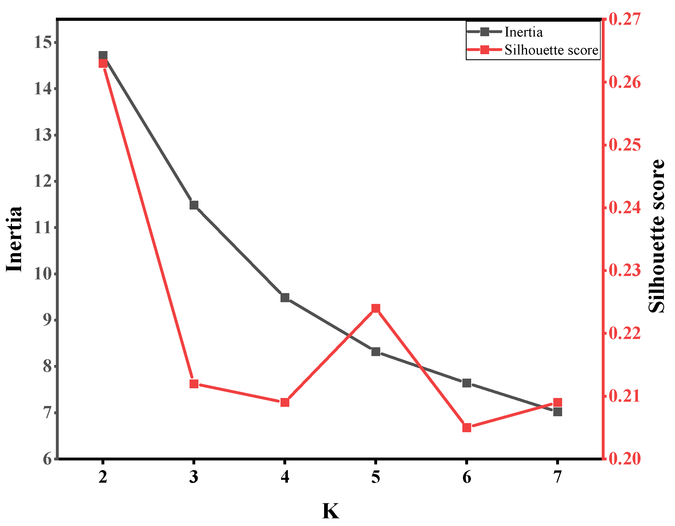
The inertia and silhouette coefficients were calculated for K from 2 to 7, as shown in Figure 9. When K = 5, the inertia is smaller and the silhouette coefficient is greater than that of K = 6 or 7. Therefore, these households are divided into five clusters. The clustering centers of the five clusters are provided in

Table 4. Cluster centers of the behavior in operating the mechanical ventilation system.

Cluster	CO2_In	PM2.5_In	T_In	PM2.5_Out	T_Out	RH_Out	H	M	Spring	Summer	Autumn	Winter
1	0.1	−0.03	−0.13	0.4	−0.06	0.07	−0.01	−0.09	0.18	−0.18	−0.06	0.08
2	0.02	−0.13	−0.2	0.14	−0.32	−0.07	−0.04	−0.05	−0.09	−0.23	−0.07	0.34
3	0.12	−0.1	0.31	0.03	0.35	0.13	0.03	−0.51	0.24	0.36	−0.33	−0.27
4	0.05	−0.12	−0.28	0.26	−0.36	−0.12	−0.03	−0.37	0.23	−0.4	−0.19	0.34
5	0.08	−0.06	−0.02	0.04	0.07	−0.01	0.04	0.16	−0.01	−0.01	0.1	−0.04

. Five motivation patterns were discovered.

(1)

Outdoor air PM_2.5 concentration-driven (Cluster 1): In this cluster, the Pearson’s correlation coefficient between the outdoor PM_2.5 concentration and the state of the mechanical ventilation system is significantly higher than the other factors (with p-value being 0.00). This indicated that households of this cluster might have been sensitive to the outdoor air quality when they chose to switch on the ventilation system.

(2)

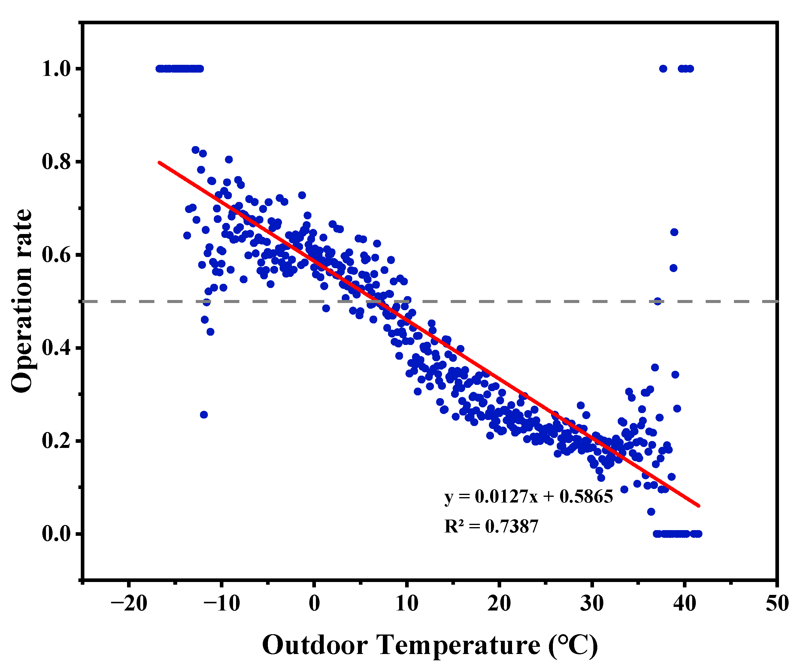
Outdoor temperature-driven (Cluster 2): In this cluster, only the Pearson’s correlation coefficient between outdoor temperature and the state of system is significant as −0.32 (absolute value greater than 0.2). Figure 10 shows the relationship between mechanical ventilation system operation rate and outdoor temperature. The 50% operation rate point and the value of the outdoor temperature at this point are marked. Thus, households of this cluster may be susceptible to outdoor temperature and tend to close the window and switch on mechanical ventilation system when outdoor temperatures drops to 6.8 °C.

(3)

Temperature and time-driven (Cluster 3): In this cluster, the Pearson’s correlation coefficients of indoor and outdoor temperature (with the status of the system) are both greater than 0.3, while that related to the month is −0.51. This indicated that these households were more inclined to switch on the system in spring and summer seasons. When the temperature increased, the air conditioner would be switched on and the windows would be closed in summer, while they were more willing to keep the system operating for ventilation.

(4)

Mixed factors-driven (Cluster 4): In this cluster, the correlation coefficient of indoor and outdoor temperature, outdoor PM_2.5 concentration and month (with the status of the system) are all significant. This suggests that the system operation behavior of this cluster could be affected by a combination of these factors.

(5)

Random behavior (Cluster 5): In this cluster, the correlation coefficients of all these factors (with the status of the system) are not significant. It could be that households in this cluster were not easily affected by these objective factors, but possibly by subjective factors, where behavior was more likely to be random.

3.2.2. Feature Selection

In order to reduce the workload of training and the modeling time, feature selection was performed on the dataset. The input feature of the model is the factor for which its absolute value of the Pearson’s correlation coefficient with the status of the ventilation system is greater than 0.1 [34].

Table 5. The selected features of the five clusters.

Cluster	Selected Features
1	PM2.5_Out, T_In, T_Out, RH_Out, H, M, spring, summer, autumn, winter
2	PM2.5_Out, T_Out, M, summer, autumn, winter
3	PM2.5_In, PM2.5_Out, T_Out, RH_Out, spring, summer, autumn, winter
4	PM2.5_ Out, T_In, T_Out, RH_Out, H, M, summer, autumn, winter
5	PM2.5_In, PM2.5_Out, spring, summer

shows the selected features of the five clusters.

3.2.3. Predictive Modeling

For the five clusters, the household dataset of each cluster is merged for next prediction modeling. The amount, imbalance rate and baseline accuracy of these datasets are listed in

Table 6. The amount, imbalance rate and baseline accuracy of datasets.

	Cluster 1	Cluster 2	Cluster 3	Cluster 4	Cluster 5	Non-Clustered
Turned off ‘0’	313,539	650,844	727,724	189,814	1,464,552	3,346,473
Turned on ‘1’	198,744	400,476	466,301	164,897	259,305	1,489,723
Imbalance rate	22.4%	23.8%	21.9%	7.0%	69.9%	38.4%
Baseline accuracy	0.612	0.619	0.609	0.535	0.85	0.692

. In this study, logistic regression and random forest are used for modeling and comparison. The selected variables were used as input features of the models and min–max normalized, which are defined in Equation (8). The hyperparameters of random forest are default values. The logistic regression estimates coefficients of the five clusters are listed in

Table 7. The logistic regression estimates coefficients of the five clusters.

Cluster	CO2_In	PM2.5_In	T_In	PM2.5_Out	T_Out	RH_Out	H	M	Spring	Summer	Autumn	Winter
1	-	-	0.0081	0.1323	−0.0489	0.0046	−0.0046	−0.2086	−0.9559	−3.0263	−2.6139	−1.6464
2	-	-	-	−0.0563	0.0409	-	-	0.132	-	−0.3494	0.5361	0.4178
3	-	−0.0091	-	0.0694	−0.0457	0.0071	-	-	−1.9499	−2.5650	−2.5533	−1.4521
4	-	-	0.0015	0.2067	0.0135	0.0093	0.0162	−0.2557	-	−4.2519	−5.1079	−4.4742
5	-	−0.0234	-	0.0554	-	-	-	-	−3.4051	−5.7716	-	-

:

$$m=\frac{x-x_{min}}{x_{max}-x_{min}}$$

(8)

where m is the transformed value, x is the original value, x_min is the minimum value in the variable column and x_max is the maximum value in the variable column.

Pipeline is a tool in machine learning. It chains multiple estimators into one and is very convenient. In this paper, pipeline was developed, which combined dataset division, classification algorithms and model evaluation [35]. Using the pipeline, it can avoid data leakage, such as disclosing some testing data in training data, and result in more accurate assessment of the generalization ability of the models.

The fitting results of logistic regression and random forest on training datasets are shown in

Table 8. The fitting results of logistic regression and random forest using the training datasets.

		Cluster 1	Cluster 2	Cluster 3	Cluster 4	Cluster 5
LR	ACC	0.784	0.665	0.717	0.785	0.874
	AUC	0.773	0.649	0.703	0.792	0.806
RF	ACC	0.999	0.994	0.994	0.999	0.998
	AUC	0.999	0.994	0.994	0.999	0.998

. Moreover, the evaluation on the predictions by logistic regression and random forest models using the test dataset are provided in

Table 9. The predictive results of logistic regression using the test datasets.

	Cluster 1	Cluster 2	Cluster 3	Cluster 4	Cluster 5	Non-Classified
ACC	0.785	0.664	0.718	0.784	0.875	0.698
AUC	0.774	0.650	0.700	0.790	0.807	0.647

and

Table 10. The predictive results of random forest using the test datasets.

	Cluster 1	Cluster 2	Cluster 3	Cluster 4	Cluster 5
ACC	0.999	0.985	0.989	0.992	0.994
AUC	0.999	0.985	0.989	0.992	0.990

, respectively. It is clearly that the accuracy of the non-clustered models is lower than those of the clustered models, supporting the fact that cluster analysis is necessary before mega-data modeling. It is notable that the higher the imbalance rate of a dataset, the worse the result of the logistic regression model, i.e., the imbalance rate of Cluster 5 is as high as 69.9%, and its ACC value of 0.698 just reached the baseline ACC value (0.692). Meanwhile, the evaluation indicators all show that the performances of random forest both on the training and test dataset are significantly better than logistic regression, and the performance is also very stable even if the dataset is very imbalanced, similarly to Cluster 5.

The predictive accuracy of the mechanical ventilation operation behavior models developed by random forest algorithm in this study is as high as 0.992 on average, which is higher than other occupant behavior models [23,25,36,37]. This may be attributed to the larger data volume and the smaller sampling interval. In addition, clustering the households before modeling should have also improved prediction accuracies.

4. Conclusions

In this study, a mechanical ventilation system of the same brand was used in 85 houses in different cities in the cold region of China, and indoor air parameters were monitored for a year. We statistically analyzed the operation duration, behavior patterns, ventilation volume and IAQ of households with different types of mechanical ventilation systems. Clustering analysis was utilized to classify households, which revealed the similarity and diversity in behaviors of different occupants. Logistic regression and random forest were used to develop models for predicting mechanical ventilation behavior with all features inputted, and their prediction results were compared. It fills the gap in the mechanical ventilation model of residential building and contributes to future studies on improving the accuracy of building simulations. The main conclusions are as follows:

(1)

About 24% households operated mechanical ventilation system nearly all day. The average daily operating system duration of the centralized system was 7.3 h/day, which was longer than that of the split system. The split system was operated more frequently. The IAQ of the households using the system almost all-day is better than that of intermittent operation.

(2)

Using K-means clustering, five patterns were discovered for the behavior of mechanical ventilation operation, including outdoor air PM_2.5 concentration-driven, outdoor temperature-driven, temperature and time-driven, mixed factors-driven and random behavior pattern.

(3)

Based on the five clusters of households, the models established by the random forest algorithm showed a better performance than that of logistic regression, and guaranteed high accuracy even when the imbalance rate of dataset was high. Therefore, the random forest algorithm can well predict the behavior in mechanical ventilation operation in residential buildings, and it can be applied in building simulation to improve the performance in future studies.

References

- Brasche, S.; Bischof, W. Daily time spent indoors in German homes–baseline data for the assessment of indoor exposure of German occupants. Int. J. Hyg. Environ. Health 2005, 208, 247–253. [Google Scholar] [CrossRef] [PubMed]
- Massey, D.; Masih, J.; Kulshrestha, A.; Habil, M.; Taneja, A. Indoor/outdoor relationship of fine particles less than 2.5 μm (PM2.5) in residential homes locations in central Indian region. Build. Environ. 2009, 44, 2037–2045. [Google Scholar] [CrossRef]
- Sundell, J. On the history of indoor air quality and health. Indoor Air 2004, 14, 51–58. [Google Scholar] [CrossRef] [PubMed]
- Abbey, D.E.; Ostro, B.E.; Petersen, F.; Burchette, R.J. Chronic respiratory symptoms associated with estimated long-term ambient concentrations of fine particulates less than 2.5 microns in aerodynamic diameter (PM2.5) and other air pollutants. J. Expo. Anal. Environ. Epidemiol. 1995, 5, 137–159. [Google Scholar] [PubMed]
- Hu, W.; Downward, G.S.; Reiss, B.; Xu, J.; Bassig, B.A.; Hosgood III, H.D.; Zhang, L.; Seow, W.J.; Wu, G.; Chapman, R.S. Personal and indoor PM2. 5 exposure from burning solid fuels in vented and unvented stoves in a rural region of China with a high incidence of lung cancer. Environ. Sci. Technol. 2014, 48, 8456–8464. [Google Scholar] [CrossRef] [Green Version]
- Dockery, D.W.; Pope, C.A.; Xu, X.; Spengler, J.D.; Ware, J.H.; Fay, M.E.; Ferris, B.G., Jr.; Speizer, F.E. An association between air pollution and mortality in six US cities. N. Engl. J. Med. 1993, 329, 1753–1759. [Google Scholar] [CrossRef] [Green Version]
- Brunekreef, B.; Holgate, S.T. Air pollution and health. Lancet 2002, 360, 1233–1242. [Google Scholar] [CrossRef]
- De Kok, T.M.; Driece, H.A.; Hogervorst, J.G.; Briedé, J.J. Toxicological assessment of ambient and traffic-related particulate matter: A review of recent studies. Mutat. Res. Rev. Mutat. Res. 2006, 613, 103–122. [Google Scholar] [CrossRef]
- Lai, D.; Qi, Y.; Liu, J.; Dai, X.; Zhao, L.; Wei, S. Ventilation behavior in residential buildings with mechanical ventilation systems across different climate zones in China. Build. Environ. 2018, 143, 679–690. [Google Scholar] [CrossRef] [Green Version]
- Zhao, L.; Liu, J. Operating behavior and corresponding performance of mechanical ventilation systems in Chinese residential buildings. Build. Environ. 2020, 170, 106600. [Google Scholar] [CrossRef]
- Zhao, Y.; Sun, H.; Tu, D. Effect of mechanical ventilation and natural ventilation on indoor climates in Urumqi residential buildings. Build. Environ. 2018, 144, 108–118. [Google Scholar] [CrossRef]
- Stabile, L.; Buonanno, G.; Frattolillo, A.; Dell’Isola, M. The effect of the ventilation retrofit in a school on CO2, airborne particles, and energy consumptions. Build. Environ. 2019, 156, 1–11. [Google Scholar] [CrossRef]
- Zhao, L.; Liu, J.; Ren, J. Impact of various ventilation modes on IAQ and energy consumption in Chinese dwellings: First long-term monitoring study in Tianjin, China. Build. Environ. 2018, 143, 99–106. [Google Scholar] [CrossRef]
- Liu, J.; Dai, X.; Li, X.; Jia, S.; Pei, J.; Sun, Y.; Lai, D.; Shen, X.; Sun, H.; Yin, H.; et al. Indoor air quality and occupants’ ventilation habits in China: Seasonal measurement and long-term monitoring. Build. Environ. 2018, 142, 119–129. [Google Scholar] [CrossRef]
- Liu, S.; Song, R.; Zhang, T. Residential building ventilation in situations with outdoor PM2.5 pollution. Build. Environ. 2021, 202, 108040. [Google Scholar] [CrossRef]
- Park, J.S.; Kim, H.J. A field study of occupant behavior and energy consumption in apartments with mechanical ventilation. Energy Build. 2012, 50, 19–25. [Google Scholar] [CrossRef]
- Kim, H.; Hong, T.; Kim, J. Automatic ventilation control algorithm considering the indoor environmental quality factors and occupant ventilation behavior using a logistic regression model. Build. Environ. 2019, 153, 46–59. [Google Scholar] [CrossRef]
- Balvedi, B.F.; Ghisi, E.; Lamberts, R. A review of occupant behaviour in residential buildings. Energy Build. 2018, 174, 495–505. [Google Scholar] [CrossRef]
- Zhang, T.; Su, Z.; Wang, J.; Wang, S. Ventilation, indoor particle filtration, and energy consumption of an apartment in northern China. Build. Environ. 2018, 143, 280–292. [Google Scholar] [CrossRef]
- Ben-David, T.; Waring, M.S. Impact of natural versus mechanical ventilation on simulated indoor air quality and energy consumption in offices in fourteen U.S. cities. Build. Environ. 2016, 104, 320–336. [Google Scholar] [CrossRef] [Green Version]
- Heydarian, A.; McIlvennie, C.; Arpan, L.; Yousefi, S.; Syndicus, M.; Schweiker, M.; Jazizadeh, F.; Rissetto, R.; Pisello, A.L.; Piselli, C.; et al. What drives our behaviors in buildings? A review on occupant interactions with building systems from the lens of behavioral theories. Build. Environ. 2020, 179, 106928. [Google Scholar] [CrossRef]
- Ren, X.; Zhang, C.; Zhao, Y.; Boxem, G.; Zeiler, W.; Li, T. A data mining-based method for revealing occupant behavior patterns in using mechanical ventilation systems of Dutch dwellings. Energy Build. 2019, 193, 99–110. [Google Scholar] [CrossRef]
- Liu, H.; Sun, H.; Mo, H.; Liu, J. Analysis and modeling of air conditioner usage behavior in residential buildings using monitoring data during hot and humid season. Energy Build. 2021, 250, 111297. [Google Scholar] [CrossRef]
- Cho, H.; Cabrera, D.; Sardy, S.; Kilchherr, R.; Yilmaz, S.; Patel, M.K. Evaluation of performance of energy efficient hybrid ventilation system and analysis of occupants’ behavior to control windows. Build. Environ. 2021, 188, 107434. [Google Scholar] [CrossRef]
- Markovic, R.; Grintal, E.; Wölki, D.; Frisch, J.; van Treeck, C. Window opening model using deep learning methods. Build. Environ. 2018, 145, 319–329. [Google Scholar] [CrossRef] [Green Version]
- Mo, H.; Sun, H.; Liu, J.; Wei, S. Developing window behavior models for residential buildings using XGBoost algorithm. Energy Build. 2019, 205, 109564. [Google Scholar] [CrossRef]
- Zhao, W.-L.; Deng, C.-H.; Ngo, C.-W. k-means: A revisit. Neurocomputing 2018, 291, 195–206. [Google Scholar] [CrossRef]
- Rousseeuw, P.J. Silhouettes: A graphical aid to the interpretation and validation of cluster analysis. J. Comput. Appl. Math. 1987, 20, 53–65. [Google Scholar] [CrossRef] [Green Version]
- Hosmer, D.W., Jr.; Lemeshow, S.; Sturdivant, R.X. Applied Logistic Regression; John Wiley & Sons: Hoboken, NJ, USA, 2013; Volume 398. [Google Scholar]
- Andersen, R.; Fabi, V.; Toftum, J.; Corgnati, S.P.; Olesen, B.W. Window opening behaviour modelled from measurements in Danish dwellings. Build. Environ. 2013, 69, 101–113. [Google Scholar] [CrossRef]
- Breiman, L. Random forests. Mach. Learn. 2001, 45, 5–32. [Google Scholar] [CrossRef] [Green Version]
- Ahmed, A.; Korres, N.E.; Ploennigs, J.; Elhadi, H.; Menzel, K. Mining building performance data for energy-efficient operation. Adv. Eng. Inform. 2011, 25, 341–354. [Google Scholar] [CrossRef]
- Hanley, J.A.; McNeil, B.J. The meaning and use of the area under a receiver operating characteristic (ROC) curve. Radiology 1982, 143, 29–36. [Google Scholar] [CrossRef] [PubMed] [Green Version]
- Zhang, R.; Nie, F.; Li, X.; Wei, X. Feature Selection with Multi-View Data: A Survey. Inf. Fusion 2019, 50, 158–167. [Google Scholar] [CrossRef]
- Olson, R.S.; Moore, J.H. TPOT: A tree-based pipeline optimization tool for automating machine learning. In Automatic Machine Learning; PMLR: Cambridge, MA, USA, 2016; pp. 66–74. [Google Scholar]
- Stazi, F.; Naspi, F.; D’Orazio, M. Modelling window status in school classrooms. Results from a case study in Italy. Build. Environ. 2017, 111, 24–32. [Google Scholar] [CrossRef]
- Yao, M.; Zhao, B. Window opening behavior of occupants in residential buildings in Beijing. Build. Environ. 2017, 124, 441–449. [Google Scholar] [CrossRef]
Figure 1.
The climate zone distribution of China and location and quantity distribution of the monitored households. Beijing, Tianjin and Hebei were the cities and province investigated. SS is the split system and CS is the centralized system; C: cold region; SC: severe cold region; M: mild region; HSCW: hot summer and cold winter region; HSWW: hot summer and warm winter region.
Figure 2.
Schematics of the (a) split and (b) centralized mechanical ventilation systems in buildings.
Figure 3.
Schematic of random forest.
Figure 4.
Pareto chart of for the monitored households.
Figure 5.
Boxplots of the average daily operating-system duration of two type mechanical ventilation systems in different seasons.
Figure 6.
Boxplots of the number of times when the two types of system are operated.
Figure 7.
Boxplots of the average ventilation volumes of the two type systems in different seasons: the split system and the centralized system.
Figure 8.
Percentage of time with hourly average indoor CO2 concentration exceeding 1000 ppm and indoor PM2.5 concentration exceeding 35 μg/m3.
Figure 9.
Inertia and silhouette score of models when K changes from 2 to 7.
Figure 10.
Relationship between mechanical ventilation system operation rate and outdoor temperature in cluster 2 households.