Article

A Fast Method for Whole Liver- and Colorectal Liver Metastasis Segmentations from MRI Using 3D FCNN Networks

1
Department of Research & Development, Division of Emergencies and Critical Care, Oslo University Hospital, 0424 Oslo, Norway
2
Department of Informatics, The University of Oslo, 0316 Oslo, Norway
3
The Intervention Centre, Oslo University Hospital, 0372 Oslo, Norway
4
Institute of Clinical Medicine, Faculty of Medicine, University of Oslo, 0450 Oslo, Norway
5
Division of Radiology and Nuclear Medicine, Oslo University Hospital, 4956 Oslo, Norway
6
Department of Physics, University of Oslo, 1048 Oslo, Norway
7
Department of Hepato-Pancreato-Biliary Surgery, Oslo University Hospital, 0372 Oslo, Norway
*
Author to whom correspondence should be addressed.
Submission received: 22 April 2022 / Revised: 13 May 2022 / Accepted: 16 May 2022 / Published: 19 May 2022
(This article belongs to the Special Issue Advance in Deep Learning-Based Medical Image Analysis)

Abstract

:
The liver is the most frequent organ for metastasis from colorectal cancer, one of the most common tumor types with a poor prognosis. Despite reducing surgical planning time and providing better spatial representation, current methods of 3D modeling of patient-specific liver anatomy are extremely time-consuming. The purpose of this study was to develop a deep learning model trained on an in-house dataset of 84 MRI volumes to rapidly provide fully automated whole liver and liver lesions segmentation from volumetric MRI series. A cascade approach was utilized to address the problem of class imbalance. The trained model achieved an average Dice score for whole liver segmentation of 0.944 ± 0.009 and 0.780 ± 0.119 for liver lesion segmentation. Furthermore, applying this method to a not-annotated dataset creates a complete 3D segmentation in less than 6 s per MRI volume, with a mean segmentation Dice score of 0.994 ± 0.003 for the liver and 0.709 ± 0.171 for tumors compared to manual corrections applied after the inference was achieved. Availability and integration of our method in clinical practice may improve diagnosis and treatment planning in patients with colorectal liver metastasis and open new possibilities for research into liver tumors.

1. Introduction

A method that can obtain liver and liver tumor segmentation from Magnetic Resonance Imaging (MRI) images in just a few seconds can benefit doctors and patients while reducing the time needed for treatment planning. Colorectal liver metastases (CRLM) develop in approximately half of patients with colorectal cancer [1], causing the second-highest number of cancer-related deaths worldwide. In 2020 it was estimated that there were more than 1.9 million new cases of colorectal metastases worldwide [2], with more than 1700 cases registered in Norway [3]. Magnetic resonance imaging (MRI) is the most sensitive method for the detection of liver metastases [4,5,6]. Such patient-specific 3D models are also utilized for 3D printing or 3D visualization using virtual or augmented reality [7].
One of the main limitations for using 3D models is the time required for annotation and segmentation from MRI scans [8,9,10]. Traditionally, segmentation is performed semi-automatically using tools such as a 3D-Slicer [11] or an ITK-snap [12]. The use of automatic methods can significantly decrease the annotation and 3D model acquiring time. Image segmentation is the most investigated area of deep learning (DL) application to medical images [13,14], and DL-based methods are increasingly proving to outperform conventional automated segmentation methods [15]. The number of research papers about DL applied to MRI liver and tumor segmentation has constantly grown over the past five years [13]. Fully connected convolutional neural networks (FCNN) represent the current gold standard for feature extraction from complex two and three-dimensional medical data. U-net [16,17], V-net [18], SegResNet [19] and HighResNet [20] are representations of such networks. While 3D U-net and V-net have already shown good literature results on liver and tumor segmentation tasks, SegResNet and HighResNet have not previously been applied to this task to the best of our knowledge.
This study aimed to develop a DL-based tool for fast and accurate MRI-based volumetric segmentation of the whole liver and liver tumors. The highlights of this study are:
  • Detection and segmentation of liver metastasis from T1 MRI in less than 7 s.
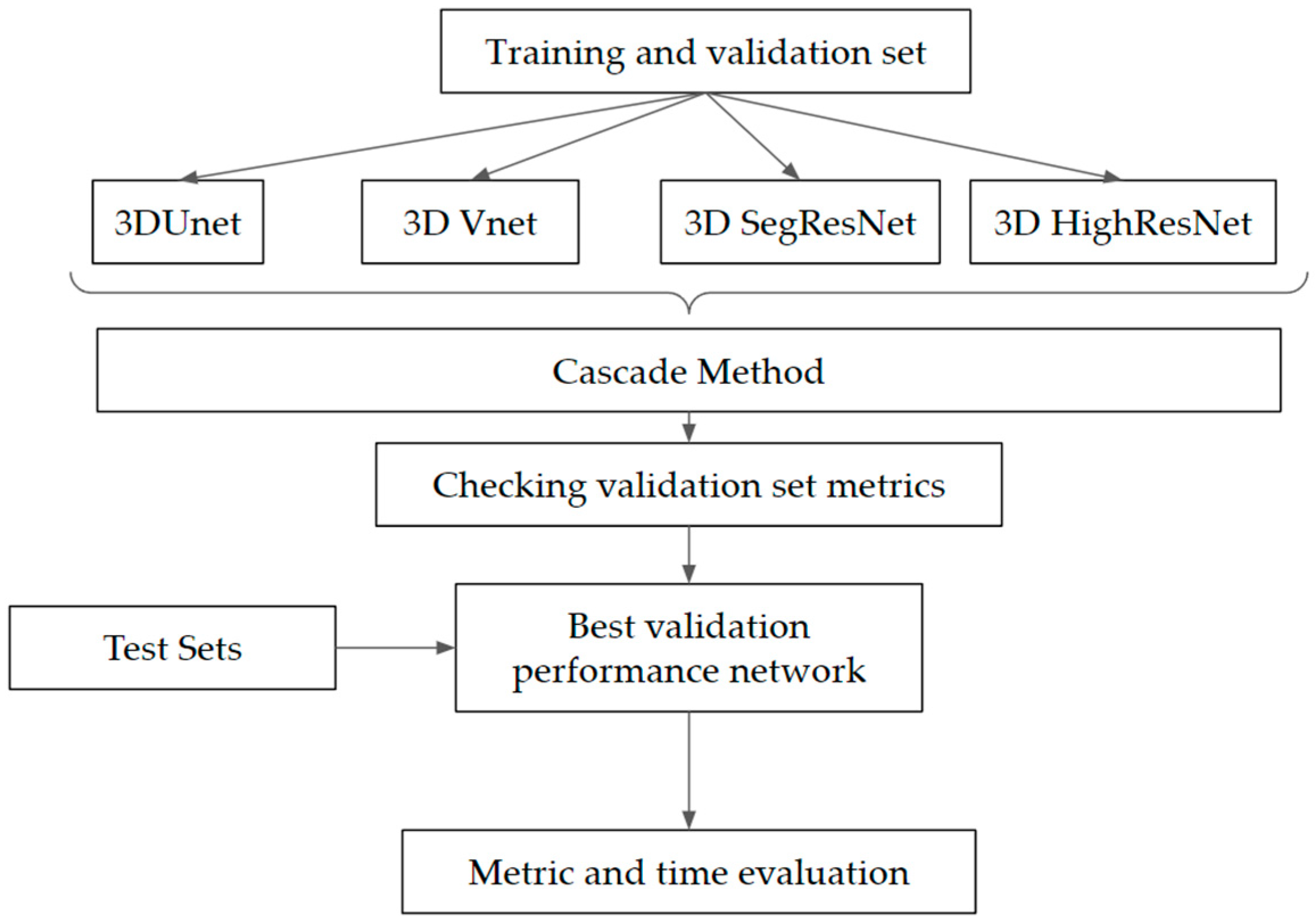
  • Creation of a cascade deep learning segmentation method based on the 3D FCNN.
  • Comparison of four FCNN segmentation networks on the inhomogeneous MRI dataset.
  • HighResNet application for the liver and liver lesion segmentation.
  • Creation of a GUI to simplify the integration of the AI tool into medical practice.
Utilizing an in-house MRI dataset, a cascade DL method based on FCNN was trained to segment CLRM and liver parenchyma from T1-weighted contrast-enhanced MRIs. In addition, this study evaluated the performance of the four most promising FCNNs within medical image segmentation on the validation set, which represents a highly unbalanced problem for segmentation with a limited number of training samples. Using the GUI, our method produced the segmentations for unannotated MRI data. Finally, we measured the time required to manually correct the obtained segmentation by our DL-based tool in order for the 3D model to be sufficient for further clinical use.

2. Literature Review

MRI is the most cost-efficient [5] and sensitive modality for liver tumor detection [6,21], though it is challenging from the perspective of automatic segmentation methods. One challenge with MRI is a variable contrast between liver and tumors depending on the sequence and the time passed after contrast injection. Any machine learning-based method requires expert annotated data for the desired task. That is why another challenge with MRI is the lack of publicly available annotated data suited to train automatic segmentation methods. Here, we used the in-house COMET dataset [22], which contains various source input data, such as machines and protocols within the T1 contrast-enhanced MRI sequence.
The use of machine learning methods for image segmentation has seen rapid growth in the past decade. In 2019 Bilic et al. released an open dataset of 131 CT cases with segmented liver and tumor segmentation [23]. The number of research papers on CT-based DL in liver and tumor segmentation has been growing [13,24]. In contrast, MRI-based DL segmentation remains a challenge due to the lack of data availability and the demand for ground truth. Several papers approached this problem using a private MRI dataset and different DL solutions [25]. The most common DL methods to segment liver and liver tumors are based on the FCNN networks [13]. The choice between 2D and 3D convolutional filters depends on the specifics of the task and on the computational resources available. In the current study, volumetric 3D MRI data were used where lesions extend across multiple slices in the 3D volume, and a 3D model approach was therefore chosen; 3D convolution is an extension of a standard 2D convolution [26] into a third dimension. The benefit of using the third dimension is utilizing 3D spatial information from MRI volumes. For example, the vessel representation in a single 2D slice could resemble a lesion; however, with 3D information, the difference between those structures may become more evident. Furthermore, 3D convolutions solve the discontinuity problem across slices of the 3D image volume [27]. Despite an increasing number of 3D U-net variations [18,28,29,30], the original 3D U-net [31] has the lowest number of parameters and shows good segmentation results on most of the medical segmentation tasks [32]. Despite the higher memory consumption, V-net [18] and SegResNet [19] show promising results in MRI segmentation tasks for brain tumor segmentation tasks. HighResNet is another 3D high-resolution convolutional network designed for volumetric image segmentation [20,33,34]. The use of dilated convolutions has already shown high-accuracy results in tumor detection on MRI brain images [35]. Compared to encode–decode networks, HighResNet has fewer training parameters (809K parameters compared to 4.8 M for 3D U-net).
The cascade approach showed promising results for tumor detection, as it helps to eliminate the background by finding the bounding box of the liver on both CT and MRI sequences [29,36,37,38,39]. Using an in-house dataset of diffusion-weighted MRI, Christ et al. segmented HCC tumors using a cascade U-net with a mean Dice score of 0.870 for liver and 0.697 for tumors [29,36,37,38,39]. Our study employed a cascade method based on four different FCNN networks to segment liver and CLRM tumors from MRI images. In contrast with the other methods, we proposed to use the network from the first stage as a weight initializer for a second network which is explained in detail in the Section 3.2.2. We aimed to reduce the training time of the second network by introducing the MRI features from one network to another.
Studies have shown that a higher Dice score for the tumor segmentation could be achieved mainly by using multiple sequences and/or contrast phases from MRI examination. For example, a Dice score of 0.91 for the liver and 0.68 for the tumor segmentation was achieved for HCC tumors using 3 T1 weighted MRI from different post contrast phases [40]. Other studies also showed that by combining the T1 weighted data with other sequences as an input for the DL networks, higher Dice scores could be achieved. For example, a Dice score of 0.83 for HCC tumor segmentation was achieved when combining T1, T2, and DW MRI sequences [41]. However, it is challenging to have the same image protocol for all patients, especially in the case of multicenter datasets such as the one used in the current study (COMET). According to the radiologist’s requirements, the image data could vary from patient to patient. Hence, only one T1 weighted contrast-enhanced image was used in our method.

3. Materials and Methods

3.1. Dataset

Model training and validation were performed in 84 T1-weighted contrast-enhanced (T1CE) MRI volumes with colorectal metastasis in the liver from the ethically approved Oslo-CoMet Study (COMET) [22]. The data were collected from seven different MR machines (Philips Medical System: Achieva, Intera, Ingenia, and SIEMENS: Aera, Avanto, Skyra, SonataVision). All images were T1CE MRI, with variations in the protocol, timings, and machine-specific image parameters. Based on domain expert ground truth (GT) annotations, there was an average of 2.8 lesions per case, with a median size of 1.574 ± 18.117 mL (range 0.021–236.23 mL). The smallest and largest lesion volumes corresponded to 0.001% and 15.61% of the total liver volume, respectively. The liver occupies, on average, 6.7 ± 2.1%, with the largest tumor of 1.15% of the total MRI volume (Figure 1).
GT segmentations were performed by two medical image processing experts with at least three years of experience in liver MRI diagnostics. Annotations from T1CE MRI were done using 3D Slicer (www.slicer.org, accessed on 15 May 2022) and ITK snap (www.itksnap.org, accessed on 15 May 2022) software tools. The number of tumors and their approximate spatial locations were confirmed by radiology reports and 2D lesion annotations (Figure 2d). The annotations were performed semi-automatically and applied to 2D slices from each volume [42], which the domain expert manually corrected as needed using a brush tool. Volumetric segmentation masks for liver and lesions were then generated from the annotations yielding non-overlapping mask values, with a background as class zero, liver parenchyma as class one, and tumors as class two.
From the segmented dataset, 60 volumes (75%) were used for training, 10 (12.5%) for validation, and 10 (12.5%) for the testing (test set #1). The data split was manual with respect to the patient and representation of all scanner variations through the subsets. The test set represents all machines that were presented in the dataset (Figure 3). Some patients had several MRI sessions that were taken into account during the split to avoid the presence of the same patient in different subsets. Four additional MRI volumes were left unannotated and used as test set #2.

3.2. The Method

A cascade DL method based on an FCNN was utilized to generate fast 3D segmentation of liver and liver tumors (Figure 5). The method utilized available functions from MONAI and Pytorch, libraries designed for medical image analysis. The deep learning model was trained using the Dell Precision 5820 Tower with NVIDIA GeForce RTX 3090 machine with 24 GB of graphics process units (GPU) memory.

3.2.1. The Network and Hyperparameters Choice

To choose the best network for 3D segmentation of liver and tumors we compared segmentation performances on the validation set of our designed cascade approach using four different FCNN networks. Our input to the network is a five-dimensional tensor, with the first two dimensions corresponding to the batch size and channel size. As we used only one MRI image, the number of input channels in this study is equal to one. All four networks have 3 output channels representing each from the predicted class. By applying voxelwise voting, the final 3D segmentation mask is obtained. The use of FCNN provides volume to volume segmentation [27]. The algorithm of the study is presented in Figure 4. All networks used in our methods were based on the convolution filter feature extraction. 3D U-net [43] and 3D V-net [18] are two FCNN networks based on 2D U-net [17], utilizing encoding and decoding paths with a skip connection between them. Both networks utilize 3D convolutions to produce the final segmentation. It requires the input feature matrix with a shape ( l , w , h , c ) where   l , w , h stand for length, width, height and c , channels, and a 3D convolutional kernel w of size w × w × w × c I × c w , where c I   , c w are the number of channels before and after the convolution. A 3D convolution output will be computed using Equation (1)
G x , y , z , n = i = 0 l 1   j = 0 w 1   h = 0 h 1   m = 1 c w i , j , k , m , n I x + i , y + j , z + k , m
By applying the stride of two, the size of the input volume is decreased by half, and using strided transpose convolutions, the size is increased back to its origin in the decoding part of the network. The main difference between the U-net and V-net architectures is the additional residual layers in the downsampling stages [18]. The number of filters of both networks begins with 16, going up to 256 at the bottleneck stage. Following the implementation proposed by the MONAI libraries, 3DV-net uses the kernel size of 5 × 5 × 5, Elu activation function, 3D batch normalization [44] and 50% of random dropout of 3D feature maps. A kernel size of 3 × 3 × 3 is used for3D U-net, along with Prelu activation function, instance batch normalization [45] and no dropout.
SegResNet is another FCNN network with a similar encoding part based on decreasing the size of the volumes using a stride of two and kernel size of 3 × 3 × 3. According to the MONAI implementation, the number of filters begins with eight and with each downsampled layer, it is multiplied by two. It is utilizing the Relu activation function in each of the blocks of the networks, group normalization [46] and without dropout. The decoder part is similar to 3D U-net implementations, with the variational autoencoder branch added by the authors [19].
HighResNet is another FCNN network that utilizes 3D convolutions to extract features from volumetric images with 3 × 3 × 3 convolution kernels. However, this network consists only of 20 convolution layers. By utilizing dilated convolutions (Equation (2)), the network avoids the encoding and decoding strategy to get the higher features from the volumes. After the first eight filters with standard 3D convolutions, the authors introduced dilated convolutions with a dilation factor r   for further feature extraction (Equation (2)). This dilation factor increases the receptive field by preserving the spatial resolution.
O x , y , z , n = i = 0 l 1   j = 0 w 1   h = 0 h 1   m = 0 c 1 w i , j , k , m , n I ( x + i r ) , ( y + j r ) , ( z + k r ) , m
To obtain the final segmentation, the final convolution layer with a 1 × 1 × 1 convolution and 160 kernels is applied. The network has a Relu activation function, batch normalization and no dropout [20].
To make a fair comparison between all four FCNN, the same hyperparameters were applied during the training and evaluation process. The choice was made using a literature search and several experiments on the training subset. Our method relied on such hyperparameters as augmentations, network parameters (loss function, optimizer, and the learning rate), and a border merging used for automatic liver cropping. During the training process, 3D image augmentations were applied to increase the data amount and variation. The input batch from the training dataset with a probability of 20% was augmented using random contrast adjustment, introducing random Gaussian smoothing and sharpening, and arbitrary affine deformations such as rotation and zooming for not more than 10% [20]. The introduction of such augmentation showed improvement in the segmentation metrics on the training dataset and aimed to overcome the overfitting problem. All hyperparameters, including loss function, optimizer, and learning rate, were defined in the configuration file, and remain constant for both networks to compare them on the validation subset. Between available loss functions and optimizers from the MONAI library, a DiceFocal Loss (Equation (3)) has shown one of the best performances on medical image segmentation tasks [47].
L D i c e F o c a l = L D i c e + L F o c a l
where L D i c e is a Dice loss (Equation (4)) and L F o c a l is Focal loss (Equation (5)). Dice loss was proposed by the authors of V-net paper [18], which was designed to deal with the imbalance of medical image data for binary problems:
L D i c e = 1 2 c = 1 C i = 1 N g i c s i c c = 1 C i = 1 N ( g i c ) 2 + c = 1 C i = 1 N ( s i c ) 2
where g i c is the ground truth binary indicator of the class label c of the voxel i , and s i c is the probability of corresponding predicted segmentation. Focal loss is the modification of standard cross-entropy loss, with a focus on misclassified examples rather than correctly classified background pixels.
L F o c a l = 1 N c C   i = 1 N ( 1 s i c ) γ g i c l o g s i c
To train the algorithm, the mean value of liver class and tumor class loss function was used by the Adam optimizer (Equation (6))
α = α 0 * ( 1 e N e ) 0.9
where α 0 is the initial learning rate, N e is a number of epochs, and e is an epoch counter [48].
After a set of experiments on a training subset, a learning rate of 1 × 10⁻⁵ and an added merging for a cropping bounding box around the liver were chosen. During the training, it was 10 voxels for each direction, and for the inference, −20 voxels was found to be the optimal value.
Due to the dataset inhomogeneity in terms of size, intensity and resolution, pre-processing was applied to normalize the input into the network and fit into the memory constraints of the GPU. Before the volumes were introduced to the network, all volumes were moved into the isotropic space using bilinear resampling. To normalize input intensities, we applied zero means and one standard deviation intensity normalization, also known as a Gaussian kernel normalization, which is a common practice for dealing with data source inhomogeneity for MRI datasets used in DL [31]. The GPU memory constrains the input image sizes for DL networks, such that the input size was 320 by 320 by 160 for 3D U-net and SegResNet, 128 by 128 by 128 for V-net, and 128 by 128 by 92 for HighResNet.
The post-processing in the final pipeline reduced the noise and achieved three-class segmentation: background, liver parenchyma, and tumors. For the liver parenchyma mask, the biggest connected component [49] was used to illuminate unconnected islands that might be predicted by the method. Within it, a binary opening was applied using a structural element of the 2-voxel-radius ball to create a final tumor 3D mask. The choice of the radius was motivated by the fact that there were no tumors smaller than 39 voxels on the training and validation datasets. Generally, small tumors are more likely to have a spherical shape [50].
V = 4 3 * π * R 3
where, V is the ball volume, and R the radius. A ball with a volume of 39 voxels3 will have a radius of 2.1 voxels according to a sphere volume formula (Equation (7)) The ball’s choice with a smaller radius (2 voxels) will remove noise while avoiding discharging potential tumor segmentation.

3.2.2. The Method Implementation Details

Since the liver and liver tumors only make up a small fraction of the total MRI volume, a cascade approach was applied to overcome the class imbalance: the method was divided into Stage 1 and Stage 2 (Figure 5). The whole MRI volume was the input in the first stage, and in the second it was cropped around the liver region volume. For each of the stages, the networks were trained separately. To integrate the method into medical use, we aimed to create a user-friendly interface for users of all backgrounds by employing the PySimpleGUI library [51].
The networks used on the first and second stages each required different data sets for training. The first network (Deep Learning Stage 1—DLS1) was trained on the full MRI volumes, with applied pre-processing on them. For the second network (Deep Learning Stage 2—DLS2), training was proceeded on manually cropped MRI volumes around the liver. DLS2 was initialized with pre-trained weights from DLS1, as both networks were trained to produce 3-class segmentation. The training was terminated when the validation loss reached a plateau and did not improve for more than 20 epochs. Network hyperparameters were preserved on both steps.
To achieve the final 3D segmentation the following five-step protocol was followed. An MRI volume was first pre-processed to match DLS1 input constraints, and the network produces the first inference. Second, the post-processed output was resampled back to the original size and spacing of the input MRI volume. Third, the coordinates of a bounding box with added merging are recorded, and the initial MRI volume was cropped using them. Fourth, the preprocessing was applied to the cropped MRI volume, and DLS2 was used to produce a second segmentation. Fifth, in the post-processing, as a final step, saved coordinates of a bounding box, where the MRI volume was cropped before, are used to insert post-processed and resampled segmentation to generate a 3D mask for the whole MRI volume. The inference process was entirely automatic and did not require any interaction with a user, except specifying the path of the input volume.

3.3. Evaluation

To inspect the final 3D segmentation mask, both quantitative and qualitative evaluation approaches were used. The quantitative evaluation included binary metrics such as the Dice coefficient, sensitivity, precision, and the number of found and missed tumors in the test set. The time required for the method to produce results and for the medical expert to manually correct obtained results (from test set #2) was measured. We present the best and worst cases in terms of the Dice metric in a form of 2D slices from volumes with the overlap of the segmentation mask from the DL method and GT in Section 4.2.2.

3.3.1. Evaluation Metrics

The Dice coefficient (Equation (8)) is the most commonly used metric in medical image segmentation, and it evaluates an overlap between GT and prediction. True-positives (TP) are voxels that were segmented positive and are also positive on the GT. False-positive (FP) and false-negative (FN) are voxels segmented as positive and negative on the prediction when they have opposite values on the GT.
D i c e = 2 * T P 2 * T P + F P + F N
We also measured the sensitivity (Equation (9)) and precision (Equation (10)) of the method applied to the liver and tumors. Sensitivity measures the percentage of true-positive voxels compared to positive samples annotated on the GT. At the same time, precision characterizes a correlation between correctly found true-positive samples to all positive samples that were predicted.
S e n s i t i v i t y = T P T P + F N
P r e c i s i o n = T P T P + F P
Due to the small number of voxels that tumors generally contain, Dice measurements may not always be reliable. Therefore, the total number of found and missed tumors per volume was measured in addition to the metrics above. Using the same approach that was taken in a Computer Tomography (CT) challenge for liver tumor segmentation, tumors were considered to be found if at least 50% of the tumor voxels were detected [23].

3.3.2. Evaluation of the Tool by a Medical Expert

A clinical expert carried out the final evaluation. Using the created Graphical User Interface (GUI), our deep learning-based method became an easy-to-use tool that produces patient-specific 3D models of the whole liver and tumors from MRI volumes. The designed workflow with the tool integration is schematically presented in Figure 3.
Each step in the procedure described in Figure 6 requires different, but sequentially complementary actions. During step (a) CET1 MRI volume was extracted from the medical dataset. The medical dataset of patients contains a lot of different modalities and extra information that cannot be processed by design solution, so it was necessary first to export MRI volume in NIFTI format and proceed with the anonymization process before putting the volume MRI into our method. On step (b), the user needs to specify the path of the input NIFTI image or the folder that contains one or multiple of them, and where to save the output segmentation. The designed GUI aimed to simplify the usability of the method. The output is a 3D segmentation, specifying the liver and tumors as class one and two, respectively. The evaluation part begins on step (c). The user has to evaluate created segmentation visually, and if needed, adjust the labels manually by relying on the professional experience and referring to radiologist annotations of tumors and their approximate location. The time required to correct and produce the final segmentation was recorded for the liver parenchyma and tumors together. On step (d), using ITK-snap or 3D Slicer visualization tools, a 3D volumetric model of the liver parenchyma and tumors was created. After a medical expert adjusted a final segmentation, the quantitative metrics of the AI output compared to the corrected version were calculated.

4. Results

4.1. Network and Method Validation Results

To compare FCNN networks, with the improvement in the proposed segmentation method by adding a cropping stage, the intermediate segmentation mask was also evaluated. Table 1 shows the segmentation results on the validation dataset using four FCNN after DLS1 with post-processing (Stage1), and after utilizing the whole pipeline proposed in Figure 5 (Full method).
From Table 1, an improvement in all metrics between Stage 1 and Stage 2 for all networks was observed. Only HighResNet was able to detect and segment the network from the full image, while three other networks detected tumors only using the full proposed method. Using only the one stage approach V-net achieved the lowest segmentation metrics for the liver segmentation with a Dice score of 0.693 ± 0.099, while HighResNet achieved the highest value within all metrics with a Dice score of 0.919 ± 0.026. After the second stage, all four networks were able to segment tumors from MRI volumes. SegResNet and HighResNet had similar performances in terms of Dice score for tumor segmentation, with higher tumor sensitivity for HighResNet of 0.915 ± 0.258, and higher precision for SegResNet of 0.692 ± 0.226. For the liver parenchyma segmentation, the best performance was achieved by HighResNet.
Inference time with loading the model, pre-and post-processing for one volume varies between the networks used. For 3D U-net, it was 6.12 ± 1.34 V-net—5.41 ± 0.99, SegResNet—6.08 ± 1.04 and for HighResNet it was 5.29 ± 0.95 s per volume.

4.2. Application on the Test Subsets

Based on the validation results, HighResNet was chosen as the final network for our method. To allow different users to utilize our tool, a user-friendly GUI was created (Figure 3, Stage B). In addition, the inference could also be performed with the command line. After the medical expert manually corrected the DL method output for test set #2, a new segmentation mask was saved in a new file and used to evaluate the method.

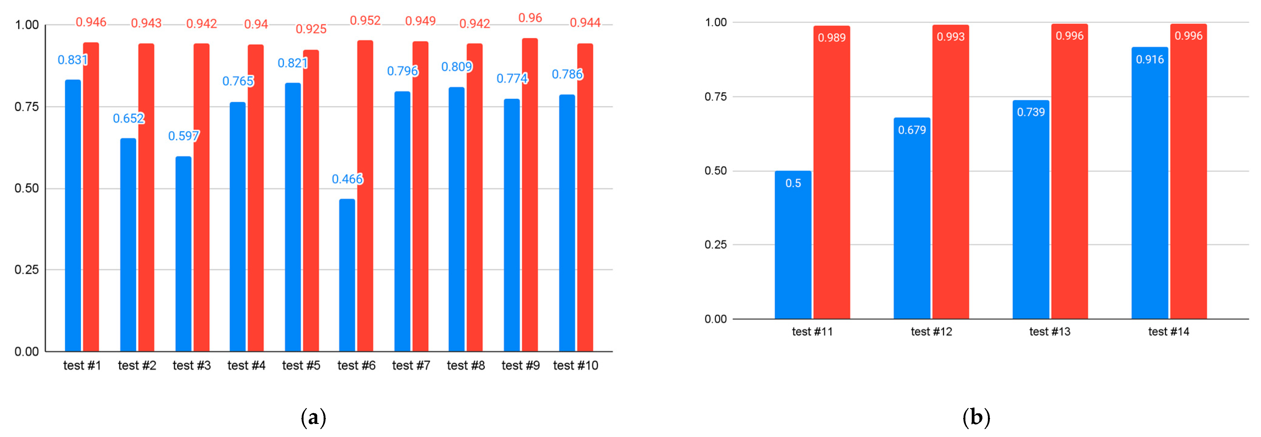
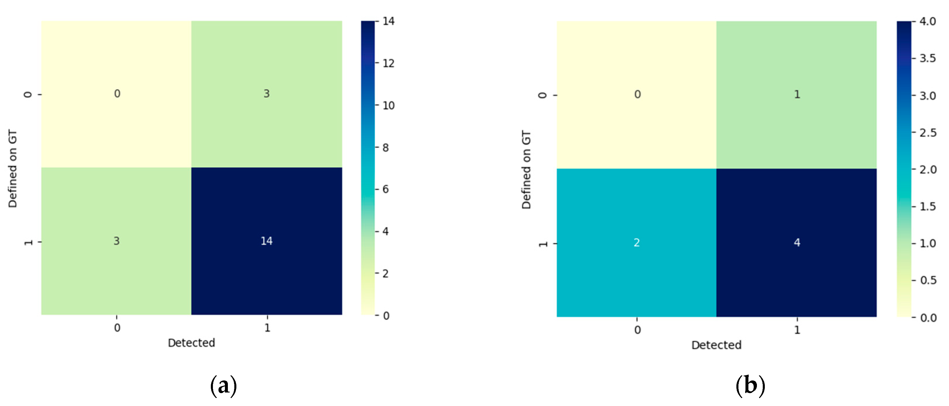
4.2.1. Quantitative Results

Segmentation metrics from obtained inferences for both test sets were presented in Table 2. Binary masks of the liver and tumors were compared to GT and expert manual corrections.
The proposed method based on the HighResNet achieved a Dice score of 0.944 ± 0.009 for the liver and 0.780 ± 0.119 for the tumor segmentation on the first test set. Out of 17 tumors defined on the GT annotation, the HighResNet found 15, while pixel-wise tumor sensitivity was 0.832 ± 0.163. The precision of 0.699 ± 0.124 and two false-positive tumors segmented by the network leads to many of false-positive pixels on the DL tumor prediction mask. On the second test subset (compared to expert manual corrections) the same method achieved a Dice score of 0.994 ± 0.003 for liver and 0.709 ± 0.171 for tumor segmentation. Among nine tumors presented in this subset, six were detected, and the average sensitivity was 0.667 ± 0.257. The method predicted no false-positive tumors, and the average precision for tumor segmentation was 0.882 ± 0.146. The average Dice score for both datasets for the liver segmentation was 0.958 ± 0.0.24, and for the CLRM tumor segmentation, the Dice score achieved was 0.724 ± 0.130.
Figure 7 presents segmentation results on each of the test samples in terms of the Dice score for the tumor and liver parenchyma.
On the test subset with GT (Figure 7a), the highest Dice score for tumors was 0.831 (test#1), and the lowest was 0.466 (test#6). For the tumors that were found, the mean Dice score was 0.780 ± 0.119. The liver segmentation Dice remained high for all cases, with the lowest result of 0.925 (test#5) and the highest of 0.960 (test#9). The average inference time was 4.82 ± 1.30 s per volume.
First, expert manual corrections were required to calculate the Dice score and other metrics on the test subset without GT (Figure 7b). The inference time to achieve DL segmentation was 5.35 ± 1.25 s per case. The average time to correct the volumes (both liver and tumor segmentation masks) was 21.15 ± 10.6 min. For the liver parenchyma, the average correction time was 10.6 ± 4.5 min. In all cases, the time required for tumor correction was similar as for all parenchyma. The longest time per volume was 32 min (test#11). The highest Dice score for tumors was 0.916 (test#14), and the lowest was 0.500 (test#11). The liver parenchyma’s lowest Dice score was 0.989 (test#11) and the highest was 0.996 (test#13 and test#14).
Figure 8 demonstrates the confusion matrix for the detected tumors by the HighresNet based methods and tumors presented on the GT. For the second test subset, the number of tumors was checked with annotations provided by the radiologist to guide and confirm expert segmentation correction.
From the boxplots, we can see that in both datasets, there were five tumors that were missed by our method. Three false-positive tumors were detected in total in both test datasets. Out of 23 lesions annotated on the dataset, 18 were segmented using our method.

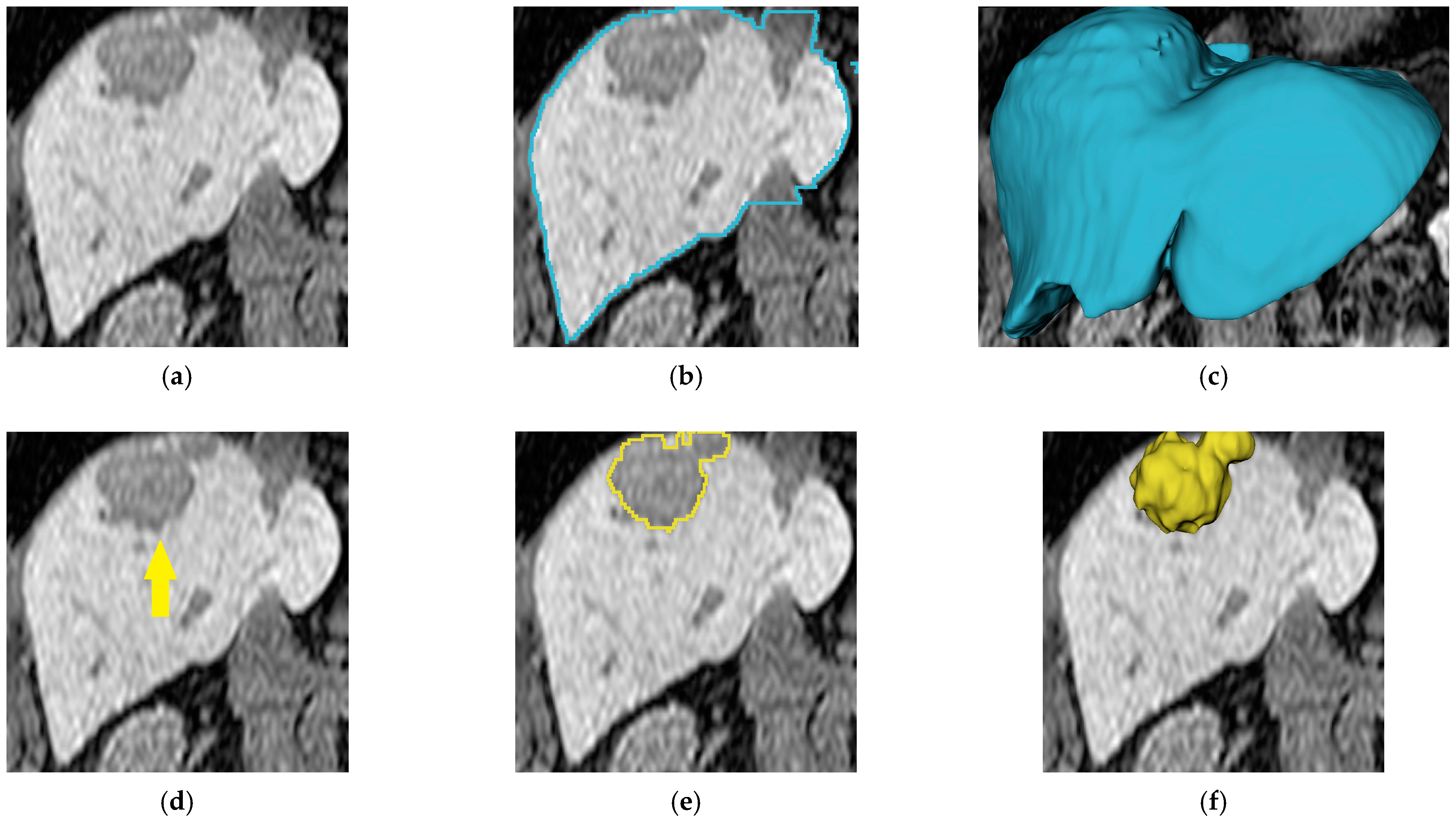
4.2.2. Qualitative Results

An overlap of DL predication and GT segmentation contours on six MRI volumes from the test set is shown in Figure 9, Figure 10 and Figure 11 to visualize the segmentation results. The first two columns correspond to different slices or views that contain tumor segmentations. A 3D model rendered in 3D Slicer for each case is presented in the third column. The red color represents DL prediction, and green is GT or segmentation corrected by a medical expert. Though on the 2D slices, both liver and tumor contours are presented, on the 3D model, only tumor segmentation is presented from both segmentation masks. A 3D model of liver parenchyma is rendered using only a DL prediction mask to make the visualization clearer and focus on the tumor segmentation.
On the two figures below, samples with the lowest and the highest tumor segmentation Dice score from the test set #1 is presented.
On the MRI volume test#3 and test#6, our method achieved a Dice score of 0.597 and 0.466 for the tumor segmentation. From Figure 9, two missed tumors on test#3 and one false-positive tumor could be observed. From the 2D slices, low over-segmentation of the liver parenchyma is presented. On test#6, the DL method has one missed tumor out of two annotated on the GT. The liver parenchyma mask is slightly under-segmented compared to a GT.
From the first row of Figure 10, we can observe that in addition to two correctly detected tumors, the DL predicted one false-positive tumor. From 2D slices, over-segmentation on the liver parenchyma and under-segmentation for the tumor borders is presented. The DL method achieved a 0.809 Dice score (test#8) in the second row, demonstrating an over-segmentation for the tumor and liver parenchyma.
On Figure 11 two MRI volumes from the second subset are presented. Consisting of a high Dice score for the liver parenchyma for all four samples from this subset, volumes shown below were selected by the lowest tumor Dice score. In addition, those two volumes (case #11, case #12) took the longest to correct for the medical expert.
One out of three tumors were missed on case test#11 (Figure 11, first row). From the 2D slices, we can see that under-segmentation on one of two detected tumors is present, while the liver parenchyma has over-segmentation. In case test#12 DL method missed two out of three tumors (Figure 11, second row). On the found tumor, over-segmentation requires manual correction from the expert. Liver parenchyma did not require a lot of modification and reached a Dice score of 0.993. The main areas requiring the most significant corrections for the liver parenchyma were borders shared with the kidney, bladder, and diaphragm.

5. Discussion

5.1. Principal Findings

The full method was trained using four cascaded FCNN networks (3D U-net, V-net, SegResNet, and HighResNet) and evaluated on the validation dataset by segmentation metrics and their improvement using the cascade approach (Table 1). All four networks improved the segmentation metrics after the cascade network was applied. The methods based on the U-net (such as 3D U-net, V-net, and SegResNet) did not contain tumors within the initial segmentation mask, which could be due to a significant class imbalance and the downsample nature of the U-net architecture. HighResNet, despite the smallest input size (128 × 128 × 92) and the lowest amount of parameters to train, was able to find tumors from the uncropped data. After the liver region was cropped, all networks could detect lesion representations from the MRI input. In the method based on the HighResNet, despite the Dice score and precision improvement, the sensitivity for the tumor class decreased from 0.948 ± 0.209 to 0.915 ± 0.258. This indicates that the detection ability of the HighResNet slightly decreased, while segmentation became more accurate. That could be due to the huge variation in the tumor shape and texture representation and the possible discharging of true-positive lesions due to overfitting on the samples from the training dataset. The lowest segmentation results were achieved by V-net, which could be also due to low liver segmentation after the first stage. Compared to other networks, this network used kernels of 5 × 5 × 5 matrix, while others are using 3 × 3 × 3 kernels; maybe changes in the filter kernel size have this influence. In general, comparing all four networks, HighResNet achieved the best Dice score with a more stable mean value for both liver and tumor segmentation. We also marked a slight reduction in time for the method based on HighResNet compared to other networks, even though all were able to produce the segmentations in less than 7 s per volume.
On the test dataset evaluation (Table 2), we observe higher tumor segmentation metrics on test set #1, with similar liver parenchyma segmentations. As in the validation subset, this could be caused by the inconsistent tumor shape and texture appearances throughout the whole dataset. Within the CLRM tumors, there are different subtypes of tumor growth patterns, and the representation of the tumors could also vary even within the same sequence and modality [52].
Visualization of our results demonstrated that the cases with the lowest Dice score network tend to predict similar tumor shapes with a bit of over-segmentation. The misclassified vessel on the first row of Figure 9 was connected to the missed tumor, which might be a reason for the method’s failure. On the second row of Figure 9, in the two tumors that were located very close to each other, the second was missed. On the other hand, in the first row of Figure 10, the network made a false-positive prediction of the completely isolated tumor while segmenting two other tumors with high accuracy. On the second row of the same figure, we can also see that the network reached the highest Dice score for liver tumor (0.809), and the 3D model and 2D contour overlap were close to each other.
In Figure 11, we can observe similarities between test#8 and test#11 (first row). The missed tumor was in close contact with another tumor that was correctly predicted and segmented by the network. In contrast, in the second row, missed tumors were located on the borders of the liver parenchyma. Despite that, the correction time for the tumors was almost the same as for the liver parenchyma due to the small volume of the tumors compared to the liver.

5.2. Comparison with Other Studies

Table 3 compares our results with previously published studies on MRI liver and liver tumor segmentation. Table 3 presented studies done on MRI data and aimed at liver or/and liver tumor segmentation.
The results of our study compare favorably with previous studies as listed in Table 3. Despite being trained on a relatively small dataset of MRI images and using only one phase from the T1 weighted modality, we achieved a Dice score for liver segmentation via HighResNet on par with the state-of-the-art.
Owler et al. solved a two-class problem using a dataset almost twice the size as in our study and achieved a slightly higher Dice score for the liver. Compared to Winther et al., the results are close in Dice scores, though being more stable in terms of standard deviation and using less data for training. Compared to other studies aiming at lesions in the liver for detection, to the best of our knowledge, we are the first to target secondary tumors such as CLRM for detection for the MRI images. Furthermore, the input to the network is just one modality compared to other research. Zhao et al. utilized three different MRI sequences from 255 patients to achieve a Dice score of 83.63 ± 2.16 for HCC tumor segmentation without liver segmentation. Our method, in contrast, requires only T1 weighted MRI to produce tumor and liver segmentation simultaneously.

5.3. Strength, Limitation, and Potential Future Application of the Study

The described solution provides high-quality segmentation of liver parenchyma and CLRM on MRI data in less than 6 s. A manual correction was applied at the end of the method before medical use, as there were cases with low sensitivity in the test set. The overall time for correcting predictions varied from 12 to 32 min and is very likely shorter than creating segmentations purely using semi-automatic tools for both parenchyma and lesions. This is especially important for the segmentation of liver parenchyma, an extensive segmentation task covering multiple slices and challenging areas in contact with other organs, requiring medical knowledge to orient in patient-specific anatomy and also a lot of care and attention to determining liver borders. As lesions in the liver are often smaller and surrounded by liver parenchyma, the corrections could be performed using purely manual tools that are not extremely time demanding.
The choice of the network to use in the final experiments was performed by the segmentation results achieved on our validation set. Although a large effort was made to find the best hyperparameters for the networks, the principal architectural components such as kernel size, batch normalization technique, and layer activation functions were predefined by the architecture implementation authors. Those parameters were different from FCNN, and maybe further experiments could increase the validation of the results. However, the aim of the study was not focused on network architecture development and modification, but rather on the application of already available DL tools into the created dataset.
Another set of experiments that could possibly improve the results would be the use of different strategies for weight initialization for the final network. It could include pre-training of the network using open medical image segmentation datasets, for example, the LITS dataset [23]. Further experiments and training on a larger dataset using the cascade method would make the method more robust and could further decrease the required time for the manual segmentation editing for the clinical use of proposed AI application.
The availability of our method to create a segmentation mask will also make it possible for further DL research in CLRM tumors within the MRI modality. Starting with a 3D segmentation by our DL method, most of the liver is already segmented. Therefore, only detecting and correcting the most significant over- and under-segmentation is left in completing the segmentation. An extension of the dataset, and training the method on more samples, will make the method more robust and increase the sensitivity of the method. Lesion segmentations produced by the presented method still require careful evaluation by a medical expert for its classification, and border adjustment. Even false-positive predictions will draw medical experts’ attention to the specific location, which might have an atypical pattern or might even be a missed lesion.
Our DL method was trained on the GT provided by just two medical experts, which can result in overfitting to their original segmentation of the MRI data. Between medical experts, the segmentation of the same structure will never have a 100% overlap due to individual human visual perception. Our future plan is to expand the study and involve more medical experts, to make the GT less biased and also to expand the method for other types of liver tumors.
Though our GUI can be used to create fast 3D segmentation for the liver parenchyma and tumors for an unannotated dataset (test set #2), the method is still limited by the type of machine on which it is trained. During the past years, 3D Slicer made several artificial intelligence (AI)-based application tools to speed up the process of medical image segmentation (AI-Assisted Annotation Server from NVIDIA [57], MONAI label from MONAI [58]). They require minimal manual initialization and show good segmentation results on CT images for liver and liver tumor segmentation tasks. In the future, we aim to integrate our trained method into this solution and make our method publicly available to increase the usability of MRI images by them.

6. Conclusions

In conclusion, our results suggest that fast and accurate liver parenchyma and liver tumor segmentation from MRI can be achieved using the HighResNet-based deep learning method. Our approach got a Dice score of 0.944 ± 0.009 for the liver and 0.780 ± 0.119 for the tumor segmentation on the annotated dataset. The time required to create and correct a clinically accurate 3D model using our method was at an average of 23 min per volume. Compared to performed annotations starting from inference by the presented approach, the DL-based segmentation received a Dice score of 0.994 ± 0.003 and 0.709 ± 0.171 for the liver and tumor. The GUI we designed for the automatic deep learning-based segmentation can be used as an assisting tool for creating a patient-specific 3D model for radiologists, which surgeons could also use for surgery planning. In the future, work will be performed to create an open code application or integrate our method with already available tools such as a 3D Slicer or ITK snap.

Author Contributions

Conceptualization, Y.K., E.P. and R.P.K.; methodology, Y.K.; software, Y.K.; validation, Y.K., E.P. and R.P.K.; formal analysis, Y.K.; investigation, Y.K.; resources, E.P.; data curation, Y.K. and E.P.; writing—original draft preparation, Y.K. and E.P.; writing—review and editing, A.B., B.E., O.J.E. and R.P.K.; visualization, Y.K. and E.P.; supervision, A.B., B.E., O.J.E. and R.P.K.; project administration, O.J.E. and R.P.K. All authors have read and agreed to the published version of the manuscript.

Funding

This research received no external funding.

Institutional Review Board Statement

The study was performed in accordance with the ethical standards of the institutional and regional ethical committee (2011/1285/REK), the 1964 Helsinki declaration and its later amendments or comparable ethical standards.

Informed Consent Statement

Informed consent was obtained from all subjects involved in the study.

Data Availability Statement

Not applicable.

Acknowledgments

This work was financially supported by the Department of Research and Development, Division of Emergencies and Critical Care, Oslo University Hospital, Rikshospitalet. The authors would like to thank Tomas Sakinis and David Aghayan for helping with dataset creation and segmentation, and Daniel Soule for the writing assistance for this paper. Special thanks to David Völgyes for help and discussions regarding the method implementations.

Conflicts of Interest

The authors declare no conflict of interest. The funders had no role in the design of the study; in the collection, analyses, or interpretation of data; in the writing of the manuscript, or in the decision to publish the results.

References

  1. Correia, M.M.; Choti, M.A.; Rocha, F.G.; Wakabayashi, G. Colorectal Cancer Liver Metastases: A Comprehensive Guide to Management. 2019. Available online: https://sciarium.com/file/463066/ (accessed on 21 October 2021).
  2. Sung, H.; Ferlay, J.; Siegel, R.L.; Laversanne, M.; Soerjomataram, I.; Jemal, A.; Bray, F. Global Cancer Statistics 2020: GLOBOCAN Estimates of Incidence and Mortality Worldwide for 36 Cancers in 185 Countries. CA Cancer J. Clin. 2021, 71, 209–249. [Google Scholar] [CrossRef] [PubMed]
  3. Cancer in Norway. 2020. Available online: https://www.kreftregisteret.no/Generelt/Rapporter/Cancer-in-Norway/cancer-in-norway-2020/ (accessed on 7 October 2021).
  4. Gavriilidis, P.; Edwin, B.; Pelanis, E.; Hidalgo, E.; de’Angelis, N.; Memeo, R.; Aldrighetti, L.; Sutcliffe, R.P. Navigated liver surgery: State of the art and future perspectives. Hepatobiliary Pancreat. Dis. Int 2022, 21, 226–233. [Google Scholar] [CrossRef] [PubMed]
  5. He, X.; Wu, J.; Holtorf, A.P.; Rinde, H.; Xie, S.; Shen, W.; Hou, J.; Li, X.; Li, Z.; Lai, J.; et al. Health economic assessment of Gd-EOB-DTPA MRI versus ECCM-MRI and multi-detector CT for diagnosis of hepatocellular carcinoma in China. PLoS ONE 2018, 13, e0191095. [Google Scholar] [CrossRef] [PubMed]
  6. Renzulli, M.; Clemente, A.; Ierardi, A.M.; Pettinari, I.; Tovoli, F.; Brocchi, S.; Peta, G.; Cappabianca, S.; Carrafiello, G.; Golfieri, R. Imaging of Colorectal Liver Metastases: New Developments and Pending Issues. Cancers 2020, 12, 151. [Google Scholar] [CrossRef] [Green Version]
  7. Pelanis, E.; Kumar, R.P.; Aghayan, D.L.; Palomar, R.; Fretland, A.; Brun, H.; Elle, O.J.; Edwin, B. Use of mixed reality for improved spatial understanding of liver anatomy. Minim. Invasive Ther. Allied Technol. 2020, 29, 154–160. [Google Scholar] [CrossRef]
  8. Kumar, R.P.; Pelanis, E.; Bugge, R.; Brun, H.; Palomar, R.; Aghayan, D.L.; Fretland, A.; Edwin, B.; Elle, O.J. Use of mixed reality for surgery planning: Assessment and development workflow. J. Biomed. Inform. 2020, 112, 100077. [Google Scholar] [CrossRef]
  9. Numminen, K.; Sipilä, O.; Mäkisalo, H. Preoperative hepatic 3D models: Virtual liver resection using three-dimensional imaging technique. Eur. J. Radiol. 2005, 56, 179–184. [Google Scholar] [CrossRef]
  10. Witowski, J.S.; Coles-Black, J.; Zuzak, T.Z.; Pędziwiatr, M.; Chuen, J.; Major, P.; Budzyński, A. 3D Printing in Liver Surgery: A Systematic Review. Telemed. E-Health 2017, 23, 943–947. [Google Scholar] [CrossRef]
  11. Gering, D.T.; Nabavi, A.; Kikinis, R.; Hata, N.; Bs, L.J.O.; Grimson, W.E.L.; Jolesz, F.A.; Black, P.M.; Wells, W.M. An integrated visualization system for surgical planning and guidance using image fusion and an open MR. J. Magn. Reson. Imaging 2001, 13, 967–975. [Google Scholar] [CrossRef]
  12. Yushkevich, P.A.; Piven, J.; Hazlett, H.C.; Smith, R.G.; Ho, S.; Gee, J.C.; Gerig, G. User-guided 3D active contour segmentation of anatomical structures: Significantly improved efficiency and reliability. NeuroImage 2006, 31, 1116–1128. [Google Scholar] [CrossRef] [Green Version]
  13. Liu, X.; Song, L.; Liu, S.; Zhang, Y. A Review of Deep-Learning-Based Medical Image Segmentation Methods. Sustainability 2021, 13, 1224. [Google Scholar] [CrossRef]
  14. Zhou, T.; Ruan, S.; Canu, S. A review: Deep learning for medical image segmentation using multi-modality fusion. Array 2019, 3–4, 100004. [Google Scholar] [CrossRef]
  15. Zhu, J.; Zhang, J.; Qiu, B.; Liu, Y.; Liu, X.; Chen, L. Comparison of the automatic segmentation of multiple organs at risk in CT images of lung cancer between deep convolutional neural network-based and atlas-based techniques. Acta Oncol. 2019, 58, 257–264. [Google Scholar] [CrossRef] [PubMed]
  16. Çiçek, Ö.; Abdulkadir, A.; Lienkamp, S.S.; Brox, T.; Ronneberger, O. 3D U-Net: Learning Dense Volumetric Segmentation from Sparse Annotation. arXiv 2016, arXiv:160606650. [Google Scholar]
  17. Ronneberger, O.; Fischer, P.; Brox, T. U-Net: Convolutional Networks for Biomedical Image Segmentation. arXiv 2015, arXiv:150504597. [Google Scholar]
  18. Milletari, F.; Navab, N.; Ahmadi, S.-A. V-Net: Fully Convolutional Neural Networks for Volumetric Medical Image Segmentation. arXiv 2021, arXiv:160604797. [Google Scholar]
  19. Myronenko, A. 3D MRI brain tumor segmentation using autoencoder regularization. arXiv 2019, arXiv:181011654. [Google Scholar]
  20. Li, W.; Wang, G.; Fidon, L.; Ourselin, S.; Cardoso, M.J.; Vercauteren, T. On the Compactness, Efficiency, and Representation of 3D Convolutional Networks: Brain Parcellation as a Pretext Task. In International Conference on Information Processing in Medical Imaging; Springer: Cham, Switzerland, 2017; Volume 10265, pp. 348–360. [Google Scholar] [CrossRef] [Green Version]
  21. Vreugdenburg, T.D.; Ma, N.; Duncan, J.K.; Riitano, D.; Cameron, A.L.; Maddern, G.J. Comparative diagnostic accuracy of hepatocyte-specific gadoxetic acid (Gd-EOB-DTPA) enhanced MR imaging and contrast enhanced CT for the detection of liver metastases: A systematic review and meta-analysis. Int. J. Colorectal Dis. 2016, 31, 1739–1749. [Google Scholar] [CrossRef]
  22. Fretland, A.; Kazaryan, A.M.; Bjørnbeth, B.A.; Flatmark, K.; Andersen, M.H.; Tønnessen, T.I.; Bjørnelv, G.M.W.; Fagerland, M.W.; Kristiansen, R.; Øyri, K.; et al. Open versus laparoscopic liver resection for colorectal liver metastases (the Oslo-CoMet study): Study protocol for a randomized controlled trial. Trials 2015, 16, 73. [Google Scholar] [CrossRef]
  23. Bilic, P.; Christ, P.F.; Vorontsov, E.; Chlebus, G.; Chen, H.; Dou, Q.; Fu, C.; Han, X.; Heng, P.; Hesser, J.; et al. The Liver Tumor Segmentation Benchmark (LiTS). arXiv 2019, arXiv:190104056. [Google Scholar]
  24. Jiang, H.; Diao, Z.; Yao, Y.-D. Deep learning techniques for tumor segmentation: A review. J. Supercomput. 2022, 78, 1807–1851. [Google Scholar] [CrossRef]
  25. Siddique, N.; Sidike, P.; Elkin, C.; Devabhaktuni, V. U-Net and its variants for medical image segmentation: Theory and applications. arXiv 2020, arXiv:201101118. [Google Scholar] [CrossRef]
  26. Deep Learning. Available online: https://www.deeplearningbook.org/ (accessed on 1 September 2021).
  27. Nie, D.; Cao, X.; Gao, Y.; Wang, L.; Shen, D. Estimating CT Image From MRI Data Using 3D Fully Convolutional Networks. In Deep Learning and Data Labeling for Medical Applications; Springer: Cham, Switzerland, 2016; pp. 170–178. [Google Scholar] [CrossRef] [Green Version]
  28. Hatamizadeh, A.; Tang, Y.; Nath, V.; Yang, D.; Myronenko, A.; Landman, B.; Roth, H.R.; Xu, D. UNETR: Transformers for 3D Medical Image Segmentation. arXiv 2021, arXiv:2103.10504. [Google Scholar]
  29. Meng, L.; Zhang, Q.; Bu, S. Two-Stage Liver and Tumor Segmentation Algorithm Based on Convolutional Neural Network. Diagnostics 2021, 11, 1806. [Google Scholar] [CrossRef] [PubMed]
  30. Oktay, O.; Schlemper, J.; Folgoc, L.L.; Lee, M.; Heinrich, M.; Misawa, K.; Mori, K.; McDonagh, S.; Hammerla, N.Y.; Kainz, B.; et al. Attention U-Net: Learning Where to Look for the Pancreas. arXiv 2018, arXiv:1804.03999. [Google Scholar]
  31. Loizou, C.P.; Pantziaris, M.; Seimenis, I.; Pattichis, C.S. Brain MR image normalization in texture analysis of multiple sclerosis. In Proceedings of the 2009 9th International Conference on Information Technology and Applications in Biomedicine, Larnaka, Cyprus, 4–7 November 2009; pp. 1–5. [Google Scholar] [CrossRef]
  32. Isensee, F.; Petersen, J.; Klein, A.; Zimmerer, D.; Jaeger, P.F.; Kohl, S.; Wasserthal, J.; Koehler, G.; Norajitra, T.; Wirkert, S.; et al. nnU-Net: Self-adapting Framework for U-Net-Based Medical Image Segmentation. arXiv 2018, arXiv:180910486. [Google Scholar]
  33. Arabi, H.; Shiri, I.; Jenabi, E.; Becker, M.; Zaidi, H. Deep Learning-based Automated Delineation of Head and Neck Malignant Lesions from PET Images. In Proceedings of the 2020 IEEE Nuclear Science Symposium and Medical Imaging Conference (NSS/MIC), Boston, MA, USA, 31 October–7 November 2020; pp. 1–3. [Google Scholar] [CrossRef]
  34. Deudon, M.; Kalaitzis, A.; Goytom, I.; Arefin, M.R.; Lin, Z.; Sankaran, K.; Michalski, V.; Kahou, S.E.; Cornebise, J.; Bengio, Y. HighRes-net: Recursive Fusion for Multi-Frame Super-Resolution of Satellite Imagery. arXiv 2020, arXiv:2002.06460. [Google Scholar]
  35. Roy, S.S.; Rodrigues, N.; Taguchi, Y.-H. Incremental Dilations Using CNN for Brain Tumor Classification. Appl. Sci. 2020, 10, 4915. [Google Scholar] [CrossRef]
  36. Christ, P.F.; Ettlinger, F.; Grün, F.; Elshaera, M.E.A.; Lipkova, J.; Schlecht, S.; Ahmaddy, F.; Tatavarty, S.; Bickel, M.; Bilic, P.; et al. Automatic Liver and Tumor Segmentation of CT and MRI Volumes using Cascaded Fully Convolutional Neural Networks. arXiv 2017, arXiv:1702.05970. [Google Scholar]
  37. Xi, X.-F.; Wang, L.; Sheng, V.S.; Cui, Z.; Fu, B.; Hu, F. Cascade U-ResNets for Simultaneous Liver and Lesion Segmentation. IEEE Access 2020, 8, 68944–68952. [Google Scholar] [CrossRef]
  38. Mourya, G.K.; Bhatia, D.; Gogoi, M.; Handique, A. CT Guided Diagnosis: Cascaded U-Net for 3D Segmentation of Liver and Tumor. IOP Conf. Ser. Mater. Sci. Eng. 2021, 1128, 012049. [Google Scholar] [CrossRef]
  39. Feng, X.; Wang, C.; Cheng, S.; Guo, L. Automatic Liver And Tumor Segmentation Of CT Based On Cascaded U-Net. In Proceedings of the 2018 Chinese Intelligent Systems Conference; Jia, Y., Du, J., Zhang, W., Eds.; Springer: Singapore, 2019; Volume 529, pp. 155–164. [Google Scholar] [CrossRef]
  40. Bousabarah, K.; Letzen, B.; Tefera, J.; Savic, L.; Schobert, I.; Schlachter, T.; Staib, L.H.; Kocher, M.; Chapiro, J.; Lin, M. Automated detection and delineation of hepatocellular carcinoma on multiphasic contrast-enhanced MRI using deep learning. Abdom. Radiol. 2020, 46, 216–225. [Google Scholar] [CrossRef] [PubMed]
  41. Zhao, J.; Li, D.; Xiao, X.; Accorsi, F.; Marshall, H.; Cossetto, T.; Kim, D.; McCarthy, D.; Dawson, C.; Knezevic, S.; et al. United adversarial learning for liver tumor segmentation and detection of multi-modality non-contrast MRI. Med. Image. Anal. 2021, 73, 102154. [Google Scholar] [CrossRef] [PubMed]
  42. Sakinis, T.; Milletari, F.; Roth, H.; Korfiatis, P.; Kostandy, P.; Philbrick, K.; Akkus, Z.; Xu, Z.; Xu, D.; Erickson, B.J. Interactive segmentation of medical images through fully convolutional neural networks. arXiv 2019, arXiv:190308205. [Google Scholar]
  43. Kerfoot, E.; Clough, J.; Oksuz, I.; Lee, J.; King, A.P.; Schnabel, J.A. Left-Ventricle Quantification Using Residual U-Net. In Statistical Atlases and Computational Models of the Heart. Atrial Segmentation and LV Quantification Challenges; Springer: Cham, Switzerland, 2019; pp. 371–380. [Google Scholar] [CrossRef]
  44. Ioffe, S.; Szegedy, C. Batch Normalization: Accelerating Deep Network Training by Reducing Internal Covariate Shift. arXiv 2015, arXiv:1502.03167. [Google Scholar]
  45. Ulyanov, D.; Vedaldi, A.; Lempitsky, V. Instance Normalization: The Missing Ingredient for Fast Stylization. arXiv 2017, arXiv:1607.08022. [Google Scholar]
  46. Wu, Y.; He, K. Group Normalization. arXiv 2018, arXiv:1803.08494. [Google Scholar]
  47. Ma, J.; Chen, J.; Ng, M.; Huang, R.; Li, Y.; Li, C.; Yang, X.; Martel, A.L. Loss odyssey in medical image segmentation. Med. Image Anal. 2021, 71, 102035. [Google Scholar] [CrossRef]
  48. Kingma, D.P.; Ba, J. Adam: A Method for Stochastic Optimization. arXiv 2014, arXiv:1412.6980. [Google Scholar]
  49. Van der Walt, S.; Schönberger, J.L.; Nunez-Iglesias, J.D.; Boulogne, F.; Warner, J.; Yager, N.; Gouillart, E.; Yu, T. scikit-image: Image processing in Python. PeerJ 2014, 2, e453. [Google Scholar] [CrossRef]
  50. Schwier, M.; Moltz, J.H.; Peitgen, H.-O. Object-based analysis of CT images for automatic detection and segmentation of hypodense liver lesions. Int. J. Comput. Assist. Radiol. Surg. 2011, 6, 737–747. [Google Scholar] [CrossRef]
  51. PySimpleGUI. Available online: https://pysimplegui.readthedocs.io/en/latest/#legal (accessed on 5 January 2022).
  52. Hugen, N.; van de Velde, C.J.H.; de Wilt, J.H.W.; Nagtegaal, I.D. Metastatic pattern in colorectal cancer is strongly influenced by histological subtype. Ann. Oncol. 2014, 25, 651–657. [Google Scholar] [CrossRef]
  53. Owler, J.; Irving, B.; Ridgeway, G.; Wojciechowska, M.; Mcgonigle, J.; Brady, S.M. Comparison of Multi-Atlas Segmentation and U-Net Approaches for Automated 3D Liver Delineation in MRI. In Medical Image Understanding and Analysis; Springer: Cham, Switzerland, 2020; pp. 478–488. [Google Scholar] [CrossRef]
  54. Winther, H.; Hundt, C.; Ringe, K.I.; Wacker, F.K.; Schmidt, B.; Jürgens, J.; Haimerl, M.; Beyer, L.P.; Stroszczynski, C.; Wiggermann, P.; et al. A 3D Deep Neural Network for Liver Volumetry in 3T Contrast-Enhanced MRI. ROFO. Fortschr. Geb. Rontgenstr. Nuklearmed. 2021, 193, 305–314. [Google Scholar] [CrossRef]
  55. Fabijańska, A.; Vacavant, A.; Lebre, M.-A.; Pavan, A.L.M.; de Pina, D.R.; Abergel, A.; Chabrot, P.; Magnin, B. U-Catchcc: An Accurate HCC Detector In Hepatic DCE-MRI Sequences Based On An U-Net Framework. In Computer Vision and Graphics; Chmielewski, L.J., Kozera, R., Orłowski, A., Wojciechowski, K., Bruckstein, A.M., Petkov, N., Eds.; Springer International Publishing: Cham, Switzerland, 2018; Volume 11114, pp. 319–328. [Google Scholar] [CrossRef]
  56. Jansen, M.J.A.; Kuijf, H.J.; Niekel, M.; Veldhuis, W.B.; Wessels, F.J.; Viergever, M.A.; Pluim, J.P.W. Liver segmentation and metastases detection in MR images using convolutional neural networks. J. Med. Imaging Bellingham Wash 2019, 6, 044003. [Google Scholar] [CrossRef] [PubMed] [Green Version]
  57. NVIDIA Clara AI-Assisted Annotation Extension—Development. 3D Slicer Community. 14 July 2019. Available online: https://discourse.slicer.org/t/nvidia-clara-ai-assisted-annotation-extension/7570 (accessed on 21 October 2021).
  58. Project MONAI. Available online: https://monai.io/ (accessed on 21 October 2021).
Figure 1. Distribution of whole liver (a)—and tumor volume (b) as a percent of total MRI volume in the expert annotated dataset.
Applsci 12 05145 g001
Figure 2. The process of dataset GT creation by the medical expert: (a) an example of a slice of MRI volume; (b) liver segmentation outline; (c) liver segmented and shown in 3D on top of MRI volumes; (d) MRI volume annotated with an arrow; (e) lesion segmentation outline; (f) lesion segmented and shown in 3D on top of MRI volumes.
Applsci 12 05145 g002
Figure 3. Distribution (percentage) of MRI data acquired on the different MRI systems included in the study: (a) Train and Validation subset (b) Test subset.
Applsci 12 05145 g003
Figure 4. Experiment setup for defining the nested FCNN network for MRI liver and tumor segmentation.
Applsci 12 05145 g004
Figure 5. Schematic representation of the used DL method used for creating 3D segmentation of liver parenchyma and tumors.
Applsci 12 05145 g005
Figure 6. Designed workflow to utilize the deep learning-based tool for 3D segmentation for liver parenchyma and tumor segmentation to create a 3D model: (a) unannotated MRI volume; (b) segmentation inference using GUI; (c) medical expert corrections and verification; (d) 3D model rendering.
Applsci 12 05145 g006
Figure 7. The Dice score achieved on test datasets with a HighResNet cascade network. The red color corresponds to the liver and blue to the tumor Dice score: (a) test set #1—compared to ground truth mask; (b) test set #2—compared to expert corrections applied after the inference.
Applsci 12 05145 g007
Figure 8. The confusion matrix for tumor detection on test datasets with a HighResNet cascade network: (a) test set #1; (b) test set #2.
Applsci 12 05145 g008
Figure 9. Two of the worst cases from the test set segmentation produced by the method in terms of the tumor Dice score: test#3—first row, test#6—second row. Green segmentation GT. Red—segmentation from the method.
Applsci 12 05145 g009
Figure 10. Two of the best cases from the test set segmentation in terms of the tumor Dice score (test#1—first row, test#8—second row). Green segmentation GT. Red—segmentation from the method.
Applsci 12 05145 g010
Figure 11. Two of the worst cases from the test set segmentation produced by the method in terms of the tumor Dice score: test#11—first row, test#12—second row. Red—segmentation from our method, Green—correction provided by the expert.
Applsci 12 05145 g011
Table 1. Results achieved on the validation set on the two stages with different FCNN networks.
NetworkSubjectSensitivityPrecisionDice
3D U-net
(Stage1)
Liver0.940 ± 0.0070.775 ± 0.1100.834 ± 0.054
Tumors000
3D U-net
(Full method)
Liver0.995 ± 0.0070.873 ± 0.1240.930 ± 0.077
Tumors0.167 ± 0.4210.051 ± 0.4120.093 ± 0.365
V-net
(Stage1)
Liver0.871 ± 0.0790.589 ± 0.1410.693 ± 0.099
Tumors000
V-net
(Stage2)
Liver0.975 ± 0.0260.762 ± 0.1470.848 ± 0.099
Tumors0.3278 ± 0.4600.385 ± 0.3820.275 ± 0.358
SegResNet
(Stage1)
Liver0.916 ± 0.0620.746∓0.1020.815 ± 0.046
Tumors000
SegResNet
(Stage2)
Liver0.992 ± 0.0080.796 ± 0.1120.879 ± 0.716
Tumors0.663 ± 0.3390.692 ± 0.2260.655 ± 0.281
HighResNet
(Stage 1)
Liver0.994 ± 0.0030.859 ± 0.0440.919 ± 0.026
Tumors0.948 ± 0.2090.351 ± 0.1560.488 ± 0.153
HighResNet
(Full method)
Liver0.988 ± 0.0080.896 ± 0.0350.942 ± 0.017
Tumors0.915 ± 0.2580.510 ± 0.1650.626 ± 0.134
Table 2. Liver parenchyma and tumor segmentation results on the test set.
NetworkSubjectSensitivityPrecisionDice
Test set #1
compared to GT
Liver0.988 ± 0.0030.903 ± 0.0190.944 ± 0.009
Tumors0.832 ± 0.1630.699 ± 0.1240.780 ± 0.119
Test set #2
compared to expert
corrections
Liver0.996 ± 0.0030.993 ± 0.0060.994 ± 0.003
Tumors0.667 ± 0.2570.882 ± 0.1460.709 ± 0.171
Table 3. Performance comparison of MRI based liver and liver tumor segmentation studies (n\a—not applicable).
Authors, YearStudy Goal and DL MethodLiver DiceTumor Dice
Owler et al., 2020
[53]
Liver segmentation using 3D U-net via T1 weighted dataset of 153 cases0.970n\a
Winther et al., 2021
[54]
Liver segmentation using V-net via T1 weighted MRI dataset of 100 patients96.0 ± 1.9n\a
Christ et al., 2017
[36]
Liver and HCC tumor segmentation via 2D U-net from DW-MRI T2-weighted dataset of 31 patients8769.7
Fabijańska et al., 2018
[55]
HCC tumor segmentation via 2D U-net from DCE-MRI dataset of 9 patientsn\a0.482
Jansen et al., 2019
[56]
Liver segmentation via FCNN network from 6 SCE MR images and tumor detection via dual pathway FCNN from SCE and DW NRI images from 121 patients0.95n\a
Sensitivity 99.8
Bousabarahet al., 2020
[40]
Liver and HCC tumor segmentation via 3D U-net from multiphasic contrast-enhanced T1-weighted MRI dataset from 174 patients0.91 ± 0.010.68 ± 0.03
Zhaoet al., 2021
[41]
HCC tumor and hemangioma segmentation via united adversarial learning framework UAL from multi modal contrast-enhances (T1-, T2-weighted and DWI) MRI images from 255 patients.n\a83.63 ± 2.16
Our methodLiver and CLRM tumor segmentation via HighResNet from a T1-weighted contrast-enhanced dataset of 80 MRI images0.958 ± 0.0240.724 ± 0.130
Publisher’s Note: MDPI stays neutral with regard to jurisdictional claims in published maps and institutional affiliations.

