
Impedance Control of Space Robot On-Orbit Insertion and Extraction Based on Prescribed Performance Method


1
School of Mechanical Engineering and Automation, Fuzhou University, Fuzhou 350108, China
2
School of Energy and Mechanical Engineering, Jiangxi University of Science and Technology, Nanchang 330013, China
*
Authors to whom correspondence should be addressed.
Appl. Sci. 2022, 12(10), 5147; https://0-doi-org.brum.beds.ac.uk/10.3390/app12105147
Submission received: 28 March 2022
/
Revised: 13 May 2022
/
Accepted: 16 May 2022
/
Published: 19 May 2022
(This article belongs to the Special Issue Robots Dynamics: Application and Control)
Abstract
:Aiming at the force position control problem of the on-orbit insertion and extraction operation of the free-floating space robot, the system dynamics model is established. According to the interaction between the end of manipulator and the environment, the second-order impedance model is established. In order to improves the calculation efficiency, the above models are reconstructed to avoid the use of acceleration signal by introducing filtering operation. This is also conducive to the application of robot actual control. Then, an estimator requiring only the system inertia matrix is designed to compensate the modeling uncertainty, external bounded disturbance and impact effect in the process of inserting and extracting. Its structure is simple and reliable. Only one control parameter needs to be adjusted, which greatly reduces the amount of calculation. Considering that the on-orbit operation of insertion and extraction is a kind of precision operation, its control system needs to have a high-quality control performance. By introducing the prescribed performance method, the tracking error is constrained within the given range and to ensure the transient performance and steady-state performance of the control system is ensured. Finally, three simulation conditions are designed, and the results are presented to verify that the proposed algorithm has a faster convergence speed compared with traditional sliding mode controller. It can achieve vertically inserting and accurate force tracking of the manipulator end.
1. Introduction
In recent years, with the increasingly expansion of space exploration activities by major aerospace countries in the world, the role of space robots has become increasingly prominent. Therefore, the research on task planning and operational control of space robot has very important engineering significance and scientific value [1,2,3,4,5]. The on-orbit service content of space robot is mainly the execution of a series of space tasks, such as docking, parking, refueling, repairing, upgrading and so on [6]. As a representative operation, the operation of insertion and insertion plays a key link function and occurs in all kinds of space tasks. Its quality of inserting and extracting would directly influence the success rate of space missions. Due to the contact and impact between space robot and targets, and the following task planning including, accurate position tracking and force tracking, it has a direct effect on the completion rate of space missions and important application value, for which worthy in-depth research [7,8,9,10,11]. So far, as a challenging subject, the theoretical research in this field is not perfect, and there is still a lot of work to be completed.
Various theories and tools are put forward to solve the problem of contact and impact. Cheng et al. [12] Analyzed the dynamic evolution process of dual arm space robot capturing non cooperative satellites, and proposed a motion stabilization control scheme based on Fuzzy . Ai et al. [13] designed a stabilizing motion force/position fuzzy sliding mode control scheme for strong impact effects in the capture process, which effectively reduced the interference caused by impact effects. Considering the influence of base, joint and arm flexibility, Fu et al. [14] carried out the dynamic analysis on a space robot capturing non-cooperative spacecraft, and designed a motion stabilization control scheme based on repetitive learning for the combination after capture. Zhu et al. [15] introduced spring compliant mechanisms at the joints of space robots to absorb impact energy, and designed a buffer compliant control scheme based on reinforcement learning which can effectively limit the impact moment at the joints within a safe range. Liu et al. [16] used the principle of dissipating energy to reduce the angular velocity of space debris before capture, which effectively protects robots from space and other physical installations. Han et al. [17] designed an elastic hemispheric gripper and a compliant control scheme in sensorless condition to reduce the impact effect during the capture process. In addition, Dai et al. [18] designed a new bionic impact resistant manipulator from the perspective of bionics, and verified its impact resistance performance through simulation and ground tests. Yan et al. [19] proposed a novel low-chattering and global-nonsingular fixed-time terminal sliding mode control strategy for fixed-time trajectory tracking for a dual-arm free-floating space robot, and its tracking accuracy of end-effector was improved to the nanoscale.
It can be found above that the researchers mainly focused on the impact effect produced by the capture of space robot to target and alleviated the impact by designing stabilization control and compliance control schemes or adding flexible parts. Nevertheless, the above research results also show that some points have not been considered, especially the issue of on-orbit operation of insertion and extraction of free-floating space robot. As a kind of precise space mission operation, on-orbit operation of insertion and extraction requires high precision of attitude control system of space robot. Due the strong nonlinear dynamic coupling of system, the relationship between force and position affects and interacts with each other. A smaller output force will not execute the operation of insertion and extraction while a bigger output force may shut down these processes. In addition, the accuracy of the position input will in turn affect the value of output force. Then, the impedance control [20,21,22,23,24] has become an effective means to solve this problem. Based on admittance control, Polverini et al. [25] proposed a control scheme for the problem of fast and sensorless peg in hole insertion of double arm robot, and completed the experimental verification on an ABB double arm robot. However, there are still considerable technical difficulties in the on-orbit operation of insertion and extraction of space robots.
In the process of inserting and extracting of space robot, there must be uncertainty caused by unmodeled error, external disturbance and violent impact, which undoubtedly improves the design difficulty of the control system. In view of the above uncertain effects, not only the traditional classical nonlinear methods such as robust control [26], sliding mode control [27], and adaptive control based on neural network [28], some new control methods and theories such as LQR method [29], MPC method [30], and reinforcement learning method [31] have been fully studied and achieved good control results in the field of aerospace. However, these controllers generally have complex design and a large calculation. Limited by the computer performance of space robot, it is worth mentioning that computational efficiency also has an important impact on the success or failure of space task. Furthermore although these controllers have achieved a high control accuracy in terms of steady-state performance (control accuracy), it fails to take into account the transient performance (error range, approaching rate, overshoot, etc.) at the same time. In addition, some of them can only ensure one or two transient performances, such as error range, convergence rate, etc. Moreover, the controlled system is expected to converge in limited task time and limited operation space according to the on-orbit task requirements. Thus, a high-quality attitude control system can largely ensure that the space manipulator and its end replaceable instruments enter the hole vertically, and reduce the adverse impact effect as much as possible. This would directly determine the success or failure of the space robot on-orbit insertion and extraction operation. The prescribed performance control method (PPC), which was jointly proposed by Greek scholars Bechlioulis and Rovithakis [32] in 2008, has attracted researchers’ extensive attention. Its core idea is to artificially set the performance envelope for the state of the controlled system, and describe the transient and steady-state performance of the controlled system through the convergence characteristics of the performance envelope function. Based on these advantages, the PPC method is widely used in the spacecraft attitude control [33,34,35].
Therefore, based on the above discussion, the force position control of free-floating space robot with output constraints is an important research direction, not to mention the unmodeled error and improving computer efficiency. The issue is actually open due to few people pay attention to it. The main contributions of this manuscript are: (1). The system dynamics model and the end second-order impedance model are established for the force position control problem of the on-orbit insertion and extraction operation of the free-floating space robot. (2). The reconstruction avoids the use of acceleration signal by introducing filtering operation. It improves the calculation efficiency and is conducive to the application of robot actual control. (3). A simple and reliable estimator requiring only the system inertia matrix is designed to compensate the modeling uncertainty, external bounded disturbance and impact effect in the process of inserting and extracting. There are only one control parameter needs to be adjusted. This also greatly reduces the amount of calculation. (4). The tracking error is constrained within the given range and the transient performance and steady-state performance of the control system is ensured by introducing the prescribed performance method. In this paper, an impedance control method in the framework of prescribed performance method is proposed for the operation of on-orbit insertion and insertion. In Section 2, the dynamics of the floating space robot with controlled attitude and uncontrolled position is modeled, and the second-order expression of the end impedance model of the manipulator is deduced. In Section 3, the equation of the established dynamic model is reconstructed and the unknown system dynamics estimator is designed for the uncertainties items in the reconstructed equation. In Section 4, under the framework of PPC method, the transient performance of space robot system is quantified, and the sliding mode controller is designed. In Section 5 three simulation conditions are designed. The following simulation results and analysis prove the effectiveness of the proposed control method, and verify that its convergence rate and error range are better than sliding mode controller.
2. Dynamic Modeling of Space Robot and Analysis of Manipulator End Impedance
2.1. Three Links Free-Floating Rigid Space Robot Model
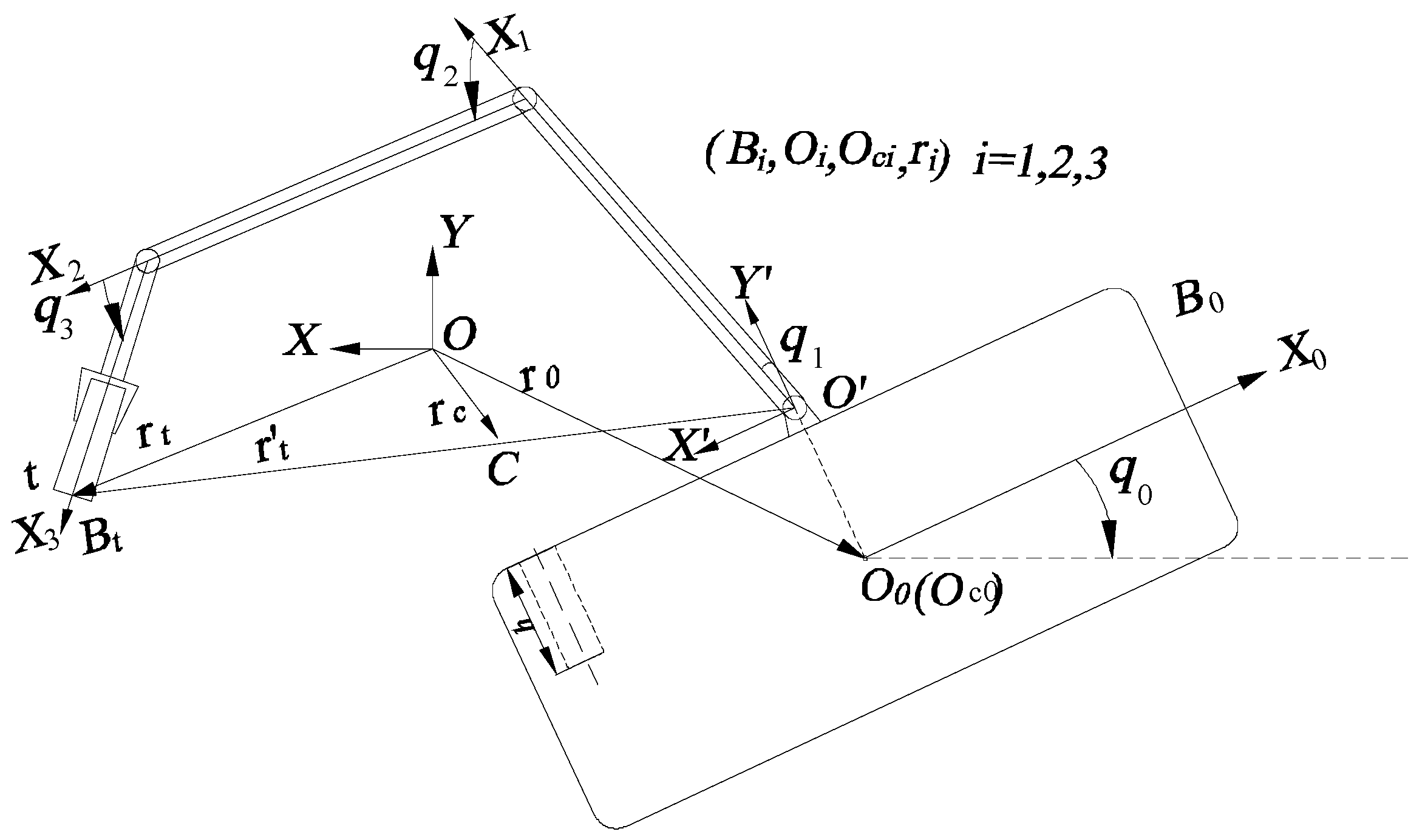
As shown in Figure 1, the free-floating three links rigid space robot consists of a carrier , three rigid arm , and , and the end replaceable instrument as the insertion and extraction parts. The global inertial coordinate system and basic coordinate system are established. Taking the base centroid and each joint center as the origin, the split contiguous coordinate system are established. In the global inertial coordinate system, the position vector of the system total centroid is defined as and the position vector of each split contiguous part centroid is defined as . The position vector of the point ‘t’ on the end of in is defined as and in is defined as . The mass of space robot carrier and each arm are defined as . Their moments of inertia are defined as , respectively. The length, mass and the moments of inertia of are defined as , and . are used to represent the length between and along the direction of . The length between and is defined as and are used to represent the length between the joint center and the centroid of arm . The insertion and extraction hole which the position of the hole center axis coincides with is located at the side of carrier and the depth is h.
The space robot generalized coordinates is defined as , where is the carrier attitude angle, , and are the joint angle, respectively. The attitude angle of end replaceable instrument is defined as . Its system dynamics equation is expressed in the following structure (the specific derivation process can be seen in the Appendix A):
where are the position, velocity and acceleration of the carrier and joint, respectively, is the symmetric positive definite mass matrix, is the column vector of centrifugal and Koch forces, is the motor rotor control torque, is the system external bounded disturbance.
2.2. The Motion Jacobian Relation
The Jacobian relation of the relative motion of the end point of the end replaceable instrument can be expressed as (the specific derivation process also can be seen in the Appendix A):
where , , and is the Jacobian matrix.
Considering the dynamics equation of space robots is position uncontrolled and attitude controlled, and the mission design requirements, the Jacobian matrix should be augmented as follow:
where , , and is the motion Jacobian matrix after being augmented.
2.3. The Impedance Model of Manipulator End
In essence, the problem of on-orbit insertion and extraction of space robots is a kind of impact dynamic between the end of robot arm and unknown environment entity. In order to avoid equipment damage and mission failure caused by violent impact between the end of manipulators and the targets, it is necessary to make compliant control for the whole process. Impedance control has a good performance in dealing with this kind of problems. The control strategy is to maintain the ideal dynamic relationship between the end-effector and the environment by adjusting the impedance parameters of the manipulator.
In general, we use the following equation to represent the terminal impedance model and the environment model:
where are the augmented desired trajectory vector of the carrier attitude, position and the attitude of the end of , and are the augmented vector of actual trajectory, , respectively, are the inertia matrix, damping matrix and stiffness matrix of manipulator, are the output force and torque, contact force and torque of end replacement instruments, are the damping matrix and stiffness matrix of environment.
According to Equation (A8), the error between the manipulator end output force and torque and the manipulator end contact force and torque can be calculated, and which can be converted to joint torques from Cartesian moments by following:
Then, if the impedance control is turned on during the on-orbit operation of the space robot, Equation (1) can be expressed as:
3. The Model Reconstruction and the Estimator of Unknown System Dynamic
In this section, the space robot system represented by Equation (1) is firstly reconstructed in which the acceleration signals are avoided being introduced to ensure transient control performance. Then based on the prescribed performance control method (PPC), the transient and steady state performance of the controlled system is quantitatively designed prior, the unknown dynamic terms are introduced to achieve precise compensation and the steady-state and transient control performance of the controller are guaranteed.
The estimator of unknown system dynamic is designed for the unknown dynamic term of reconstructed equation, that is and .
According to the space robot system represented by Equation (1), it is obviously that the acceleration signals are introduced by . Reconstruct the Equation (1), then we have:
where is the vector without acceleration signals, is the lumped unknown dynamic items that consists of centrifugal and Koch forces and external bounded disturbance.
The system represented by Equation (1) can be converted to Equation (7) by means of Equation (8):
where contains the acceleration signals .
To avoid using directly and in the estimation of , filter operations are introduced, then we have:
where , , and are the filter variables of , , and , respectively, is the scalar filtering constant.
Substituting Equation (9) into Equation (8), the space robot system can be rewritten as:
Then, function G is defined as follows:
Lemma 1.
Suppose V is any given continuous Lyapunov function, if it satisfies , and, the system is uniformly global bounded, which means the system is stable.
Define the Lyapunov function, and take derivative of as follows:
According to Assumption A1, we have: . Then based on Young’s inequality, the simplification results are obtained as follows:
Therefore, Lemma 1 is proved, are bounded. converges exponentially and its radius of convergence is obtained by solving Equation (21):
In addition, the radius convergence of is obtained as follows:
The unknown system dynamic estimator is designed as following:
The is defined as estimated error by Equations (11) and (16):
When taking derivative of Equation (17), we have:
Similarly, according to Lemma 1, Lyapunov function is defined as , when taking derivative of , we have:
Then the estimation error convergence boundary is:
Therefore, when .
4. The Design of Controller
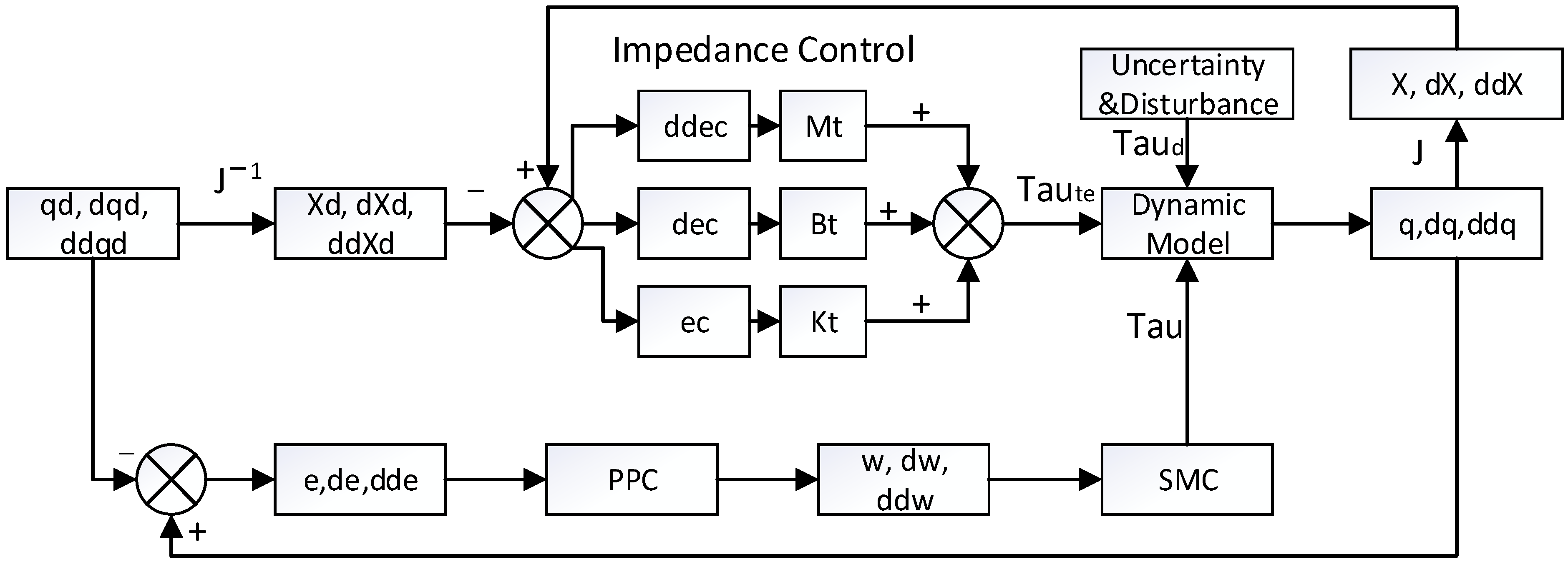
The PPC method can quantitatively describe the transient and steady-state performance of the controlled system. Under the framework of PPC, its controller design strictly follows three key steps: prescribed performance constraints, space equivalent mapping and Nonlinear controller design. This section mainly describes how the controller is designed. The above steps of controller design are mainly described in this section. The control block diagram of space robot system is as Figure 2 follows:
4.1. Prescribed Performance Constraints
Before formally designing the prescribed performance function constraints, we first analyze the insertion and extraction process of space robot represented by the following schematic diagram. We can find that the operation takes place in inertial space and the central axis of replaceable instruments coincides with the central axis of insertion hole. Therefore, we need to design the desired trajectory of the manipulator end in Cartesian space.
In order to avoid sudden change of friction during the task, and ensure the operation is successfully realized with smooth process. Then, according to Figure 3, combine the later part of the findings described in the previous paragraph and schematic diagram, and are designed as:
Combined with Equations (21) and (A8), the manipulator end desired trajectory of insertion and extraction are obtained as:
where, the specific expressions of and will be given in Section 5.
Then, the tracking error in coordinates system is obtained as:
For the fully space robot Equation (23), the tracking error in joint space is defined as follow:
where is desired trajectory and velocity.
Referring to Equation (11), we have the following:
In the first step of PPC method, it usually applies a performance function to limit the upper and lower bounds of the system state. The performance function needs to meet the following two properties:
- (1)
- It is time dependent and monotonically decreasing.
- (2)
- It is continuously differentiable.
The following exponential function is chosen as the performance function:
where are the default performance parameters. is the default performance function initial value and is the stable value. is related to the convergence rate of the .
After processing by default performance function, it usually applies a set of inequalities to limit the upper and lower bounds of the system state, which is quantified as:
where is default boundary parameters.
Additional upper and lower bound constraints are introduced for the control system to ensure transient and steady state performance of the system. However, this also makes the design of the corresponding controller more difficult. For the convenience of controller design, the nonlinear system represented by Equation (33) needs to be unconstrained.
4.2. Space Equivalent Mapping
In this part, a homeomorphic mapping function needs to be found in being used to achieve peer conversion from performance constrained space to unconstrained space. First, the error function is normalized that can be written as:
where is the equivalent tracking error and .
A tangent function is chosen to use for homeomorphic mapping, which can be written as:
where is the equivalent tracking error.
Then, based on Equation (29), the switching error can be calculated as:
4.3. Nonlinear Controller Design
In the third step of PPC, sliding mode control was chose for its good advantage in dealing with nonlinear problems. Now we define the sliding mode surface as follows:
where is control constant.
Take the derivative of the sliding surface s with respect to time, we have:
where is a bounded variable, which satisfies , and can be written as:
According to Equation (33), a sliding mode controller containing unknown dynamic terms can be designed as follows:
where is the control gain coefficient.
Substitute Equation (34) into Equation (32), we have:
Now, we have obtained the sliding mode controller which only includes the inertial matrix of the space robot system represented by Equation (7). For this controller, the following is chosen as Lyapunov function and which can be written as:
The follow Equation (37) is obtained when taking the derivative of Equation (36):
where is the minimum eigenvalue of , and is the maximum eigenvalue of , , .
According to Lemma 1, when and , there are and, which indicates that the system is stable.
5. Simulation Analysis
The three-link single-arm rigid space robot system shown in Figure 1 is used as an example for simulation and analysis. The model parameters of space robot and the end replaceable instrument are as follows:
Then, three simulation conditions are designed: the insertion on front side of carrier without a sudden change in friction, the insertion on front side of carrier with a sudden change in friction and the extraction on front side of carrier without a sudden change in friction. The details of these working conditions and simulation results are described in the following sections.
5.1. Details and Results of the First Simulation Condition
Suppose that the friction in insertion only exists along its direction and remain unchanged. Then, an ideal physical process of on-orbit insertion operation can be described as:
The end replaceable instrument is tightly held by the manipulator end that can be seen as a rigid body overall (hereinafter referred to as space robot end). Switching off the impedance controller, the space robot end is controlled to move directly above the insertion position, and its attitude is adjusted to make it perpendicular to the hole plane. The next, switching on the impedance controller, the output force of the space robot end are gradually increased to expected value before the impact happens. Then, the space robot begins to execute the on-orbit insertion operation.
The settings of the condition are: the insertion position on front side of carrier in the base-coordinate system are ; the initial attitude of the carrier, the initial position and attitude of space robot end, respectively, are ; the friction are ; the simulation step is set to 0.001 s and the total time is 13 s.
According to the above description, the expected trajectory and output force are, respectively, designed as:
The default performance function is ; the upper and lower bounds are set to and ; the control gains are ; the filter coefficient of the dynamic estimator of the unknown system is .
What’s more, a control group using sliding mode control (SMC) is set up to verify the effectiveness of the proposed prescribed performance control algorithm (PPC).
The simulation programs are executed on MATLAB R2020b and the simulation results are shown in the following figures.
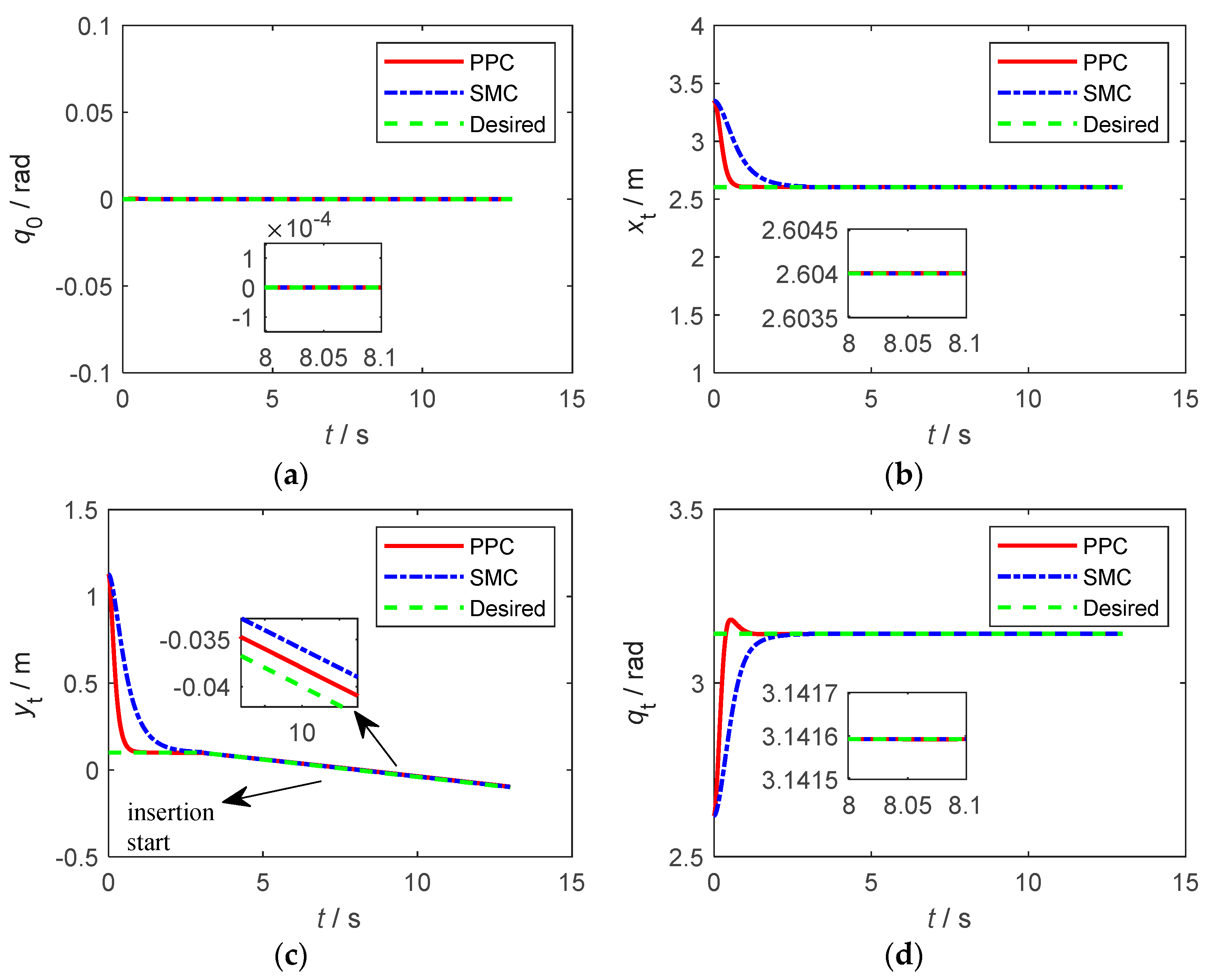
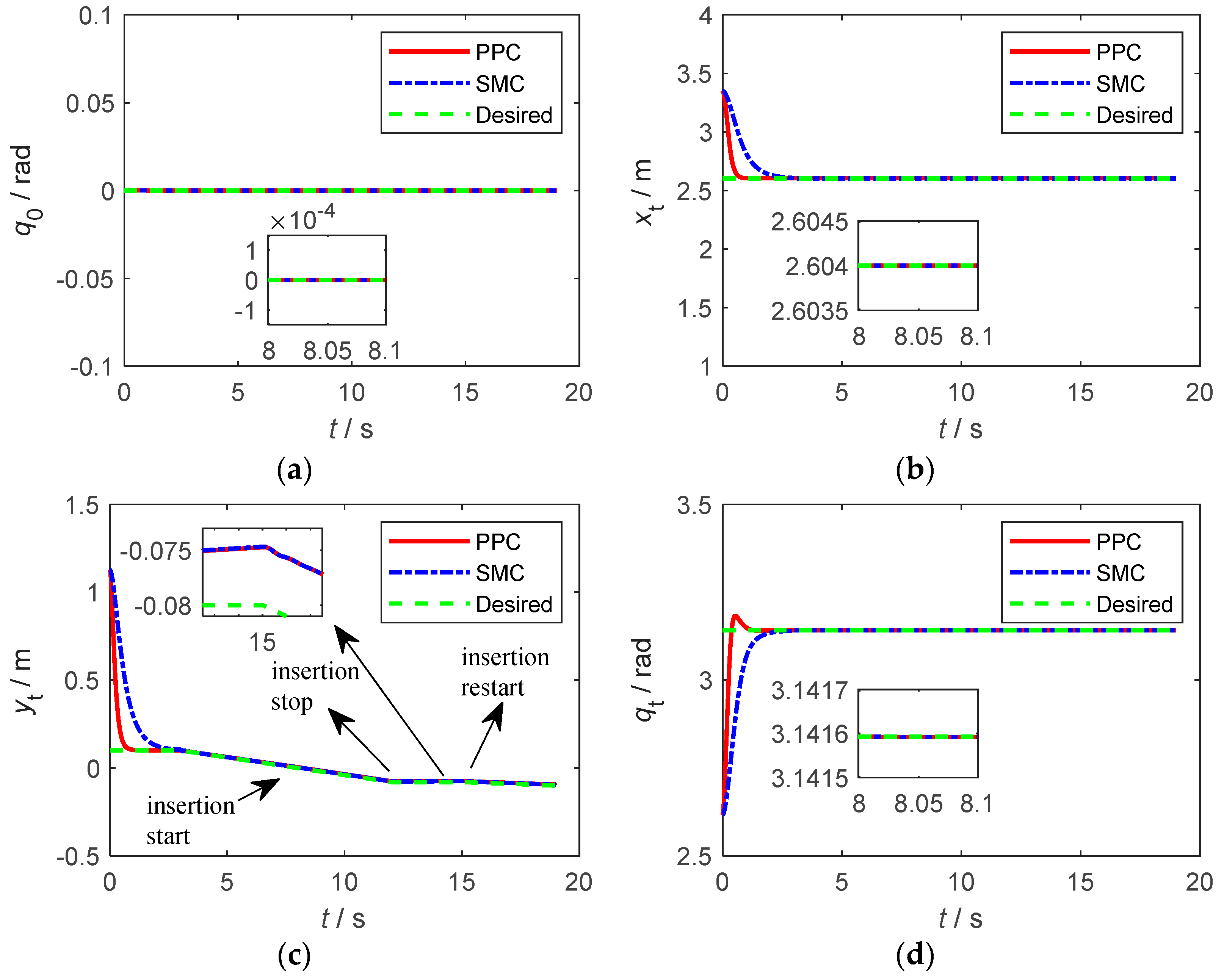
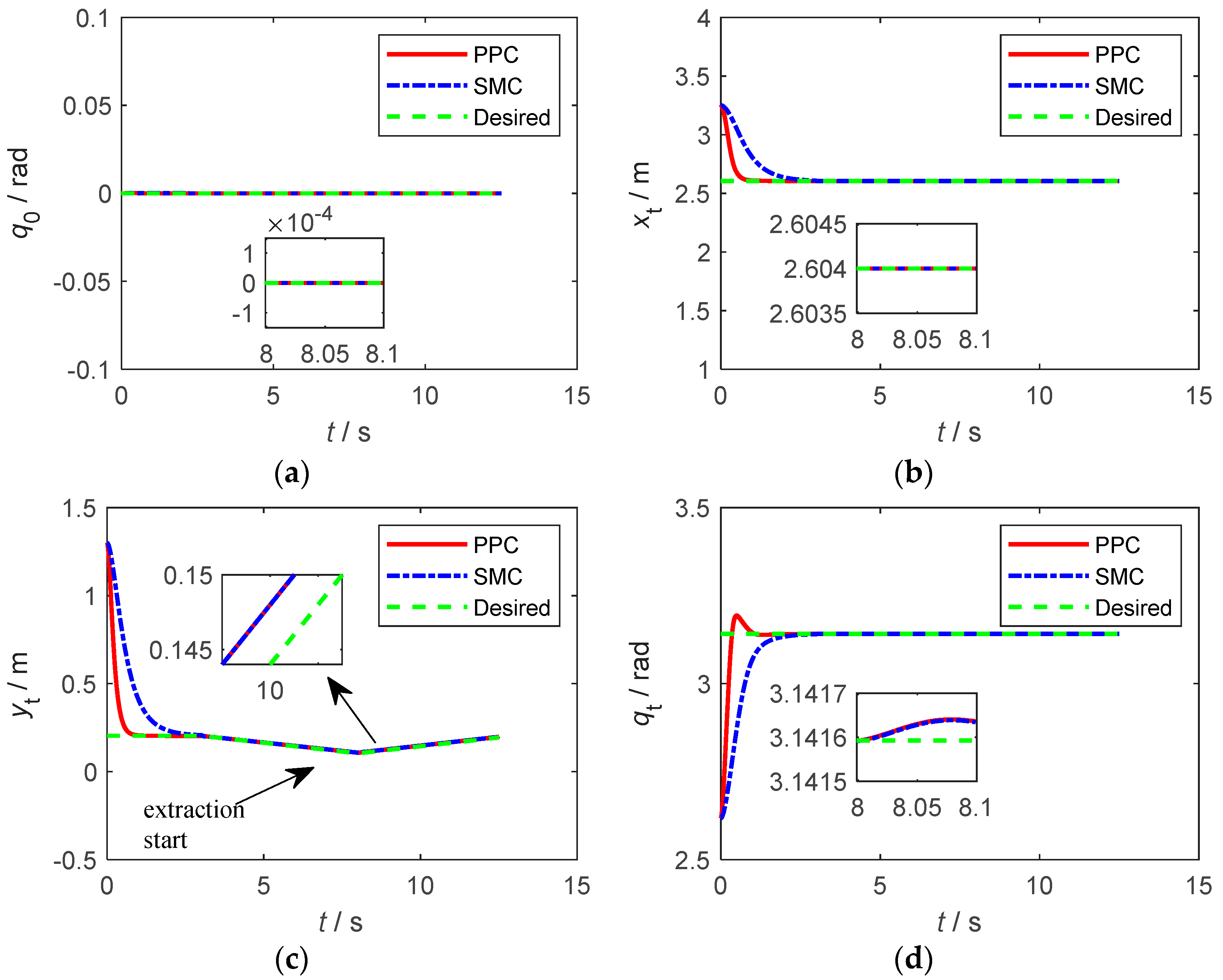
Figure 4a–d, respectively, are the carrier attitude, the space robot end position and attitude trajectory tracking curve of on-orbit insertion operation. Figure 4a,d correspond to the description in Section 4.1. The trajectory where the three curves coincide in Figure 4b correspond to the vertical trajectory in Figure 5 which represents the X-direction position of the insertion hole. From these results, it can be seen that the space robot end is controlled to move to the insertion hole with less than 0.0001 rad control accuracy of carrier and manipulator end attitude and less than 0.0001 m control accuracy of the X-direction position of manipulator end. Figure 4c indicates the change process of an ideal insertion in the direction of inserting. The space robot end is controlled to move from its initial position to the directly above the insertion position in 0~3 s. In 3~8 s, the space robot end adjusts its attitude and move to the insertion hole position. Then, in 8~13 s, the insertion operation is executed.
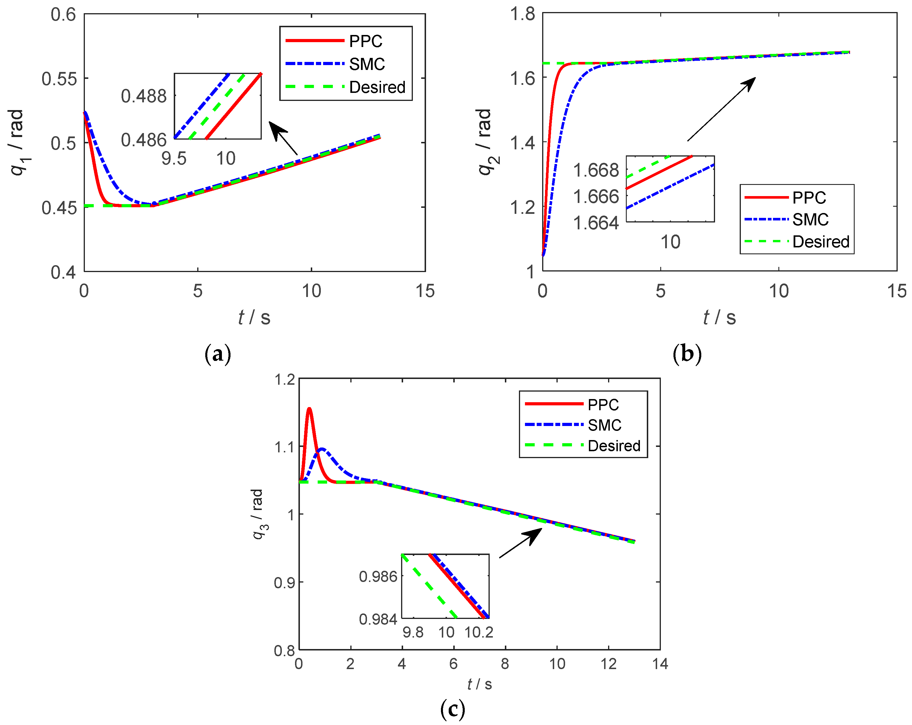
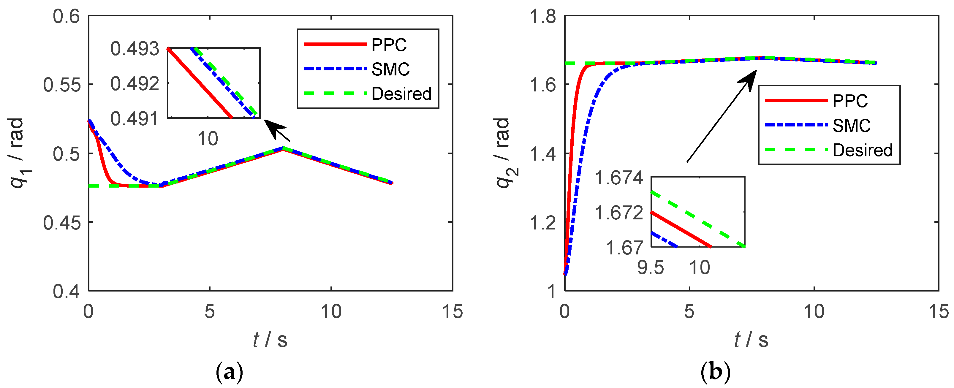
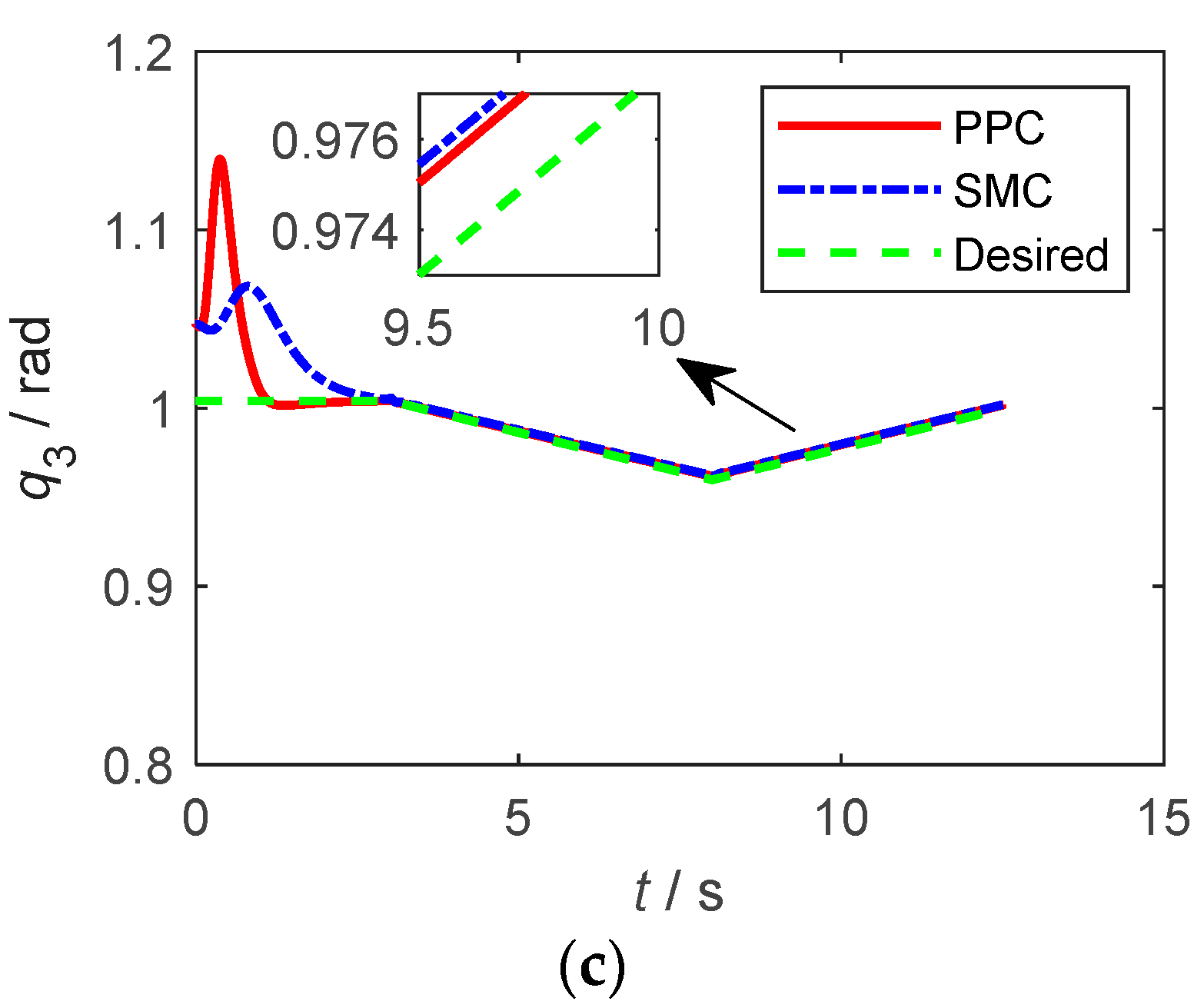
Figure 5 shows the joint trajectory tracking curve.
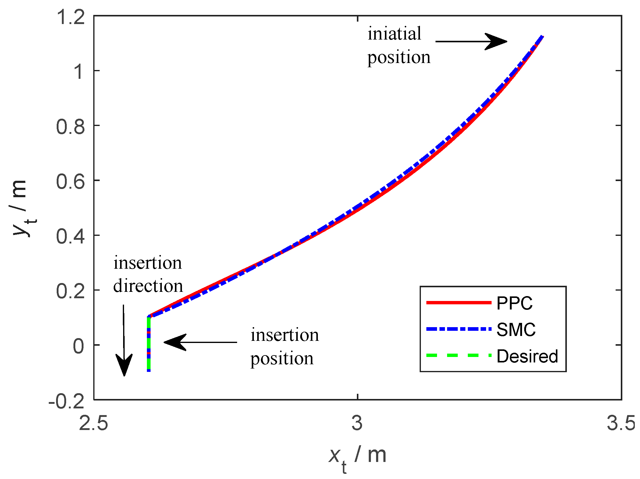
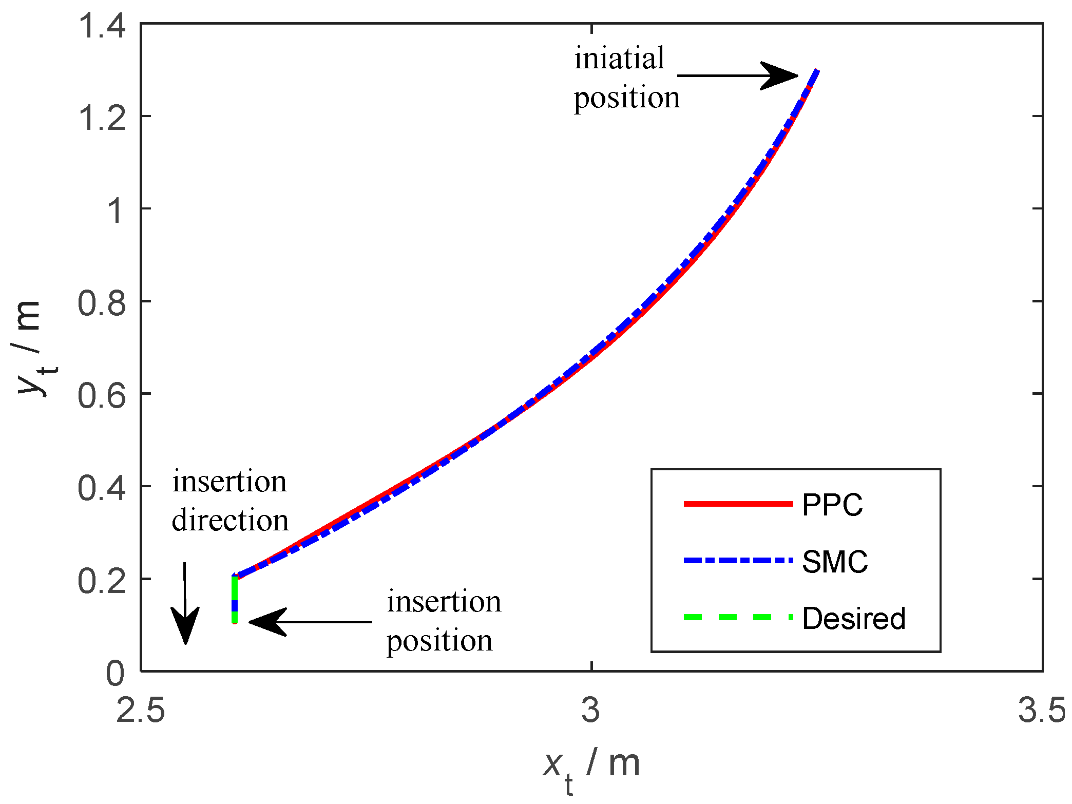
Figure 6 shows the two-dimensional trajectory in basic coordinate system . The initial position of the space robot end and the insertion position are marked in the image.
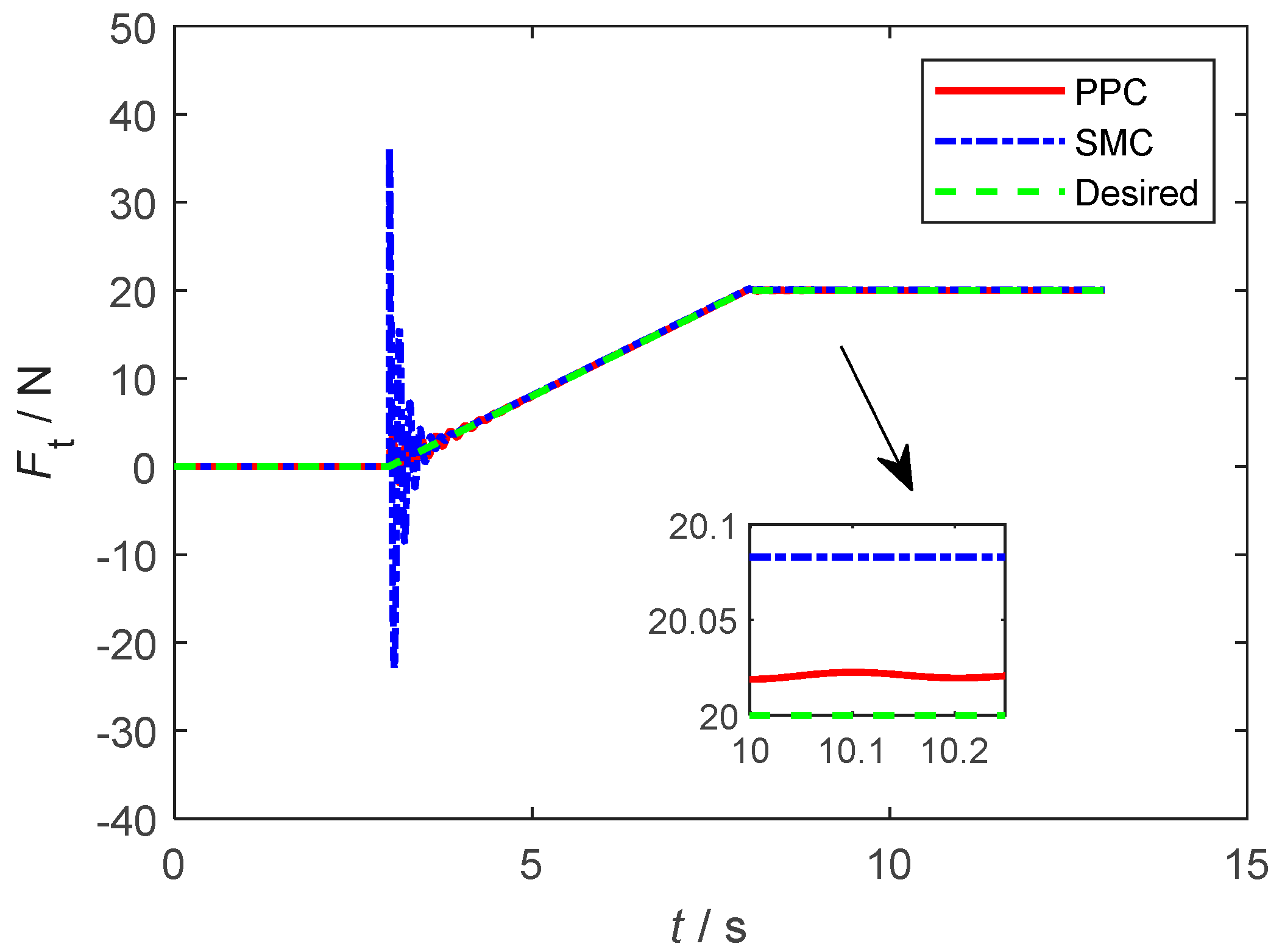
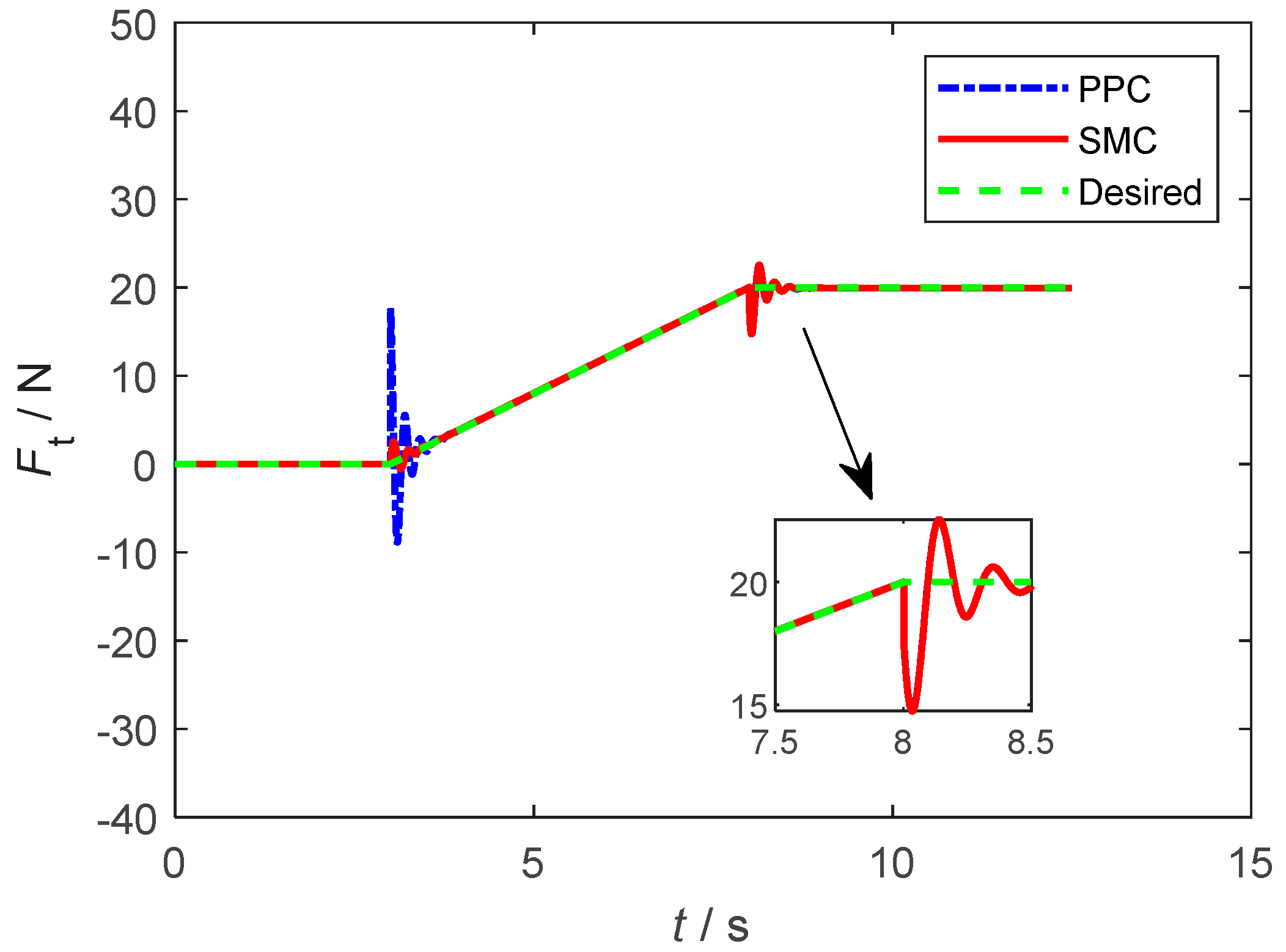
The control condition illustrated in Figure 7 is in accordance with the description in the beginning of this subsection. The space robot end impedance control is switched off in 0~3 s and switched on in 3~13 s. In 3~8 s, the output forces of space robot end are increased to 20 N gradually and linearly. Then, in 8~13 s, the output forces remain the expected value and the space robot begin to perform the operation.
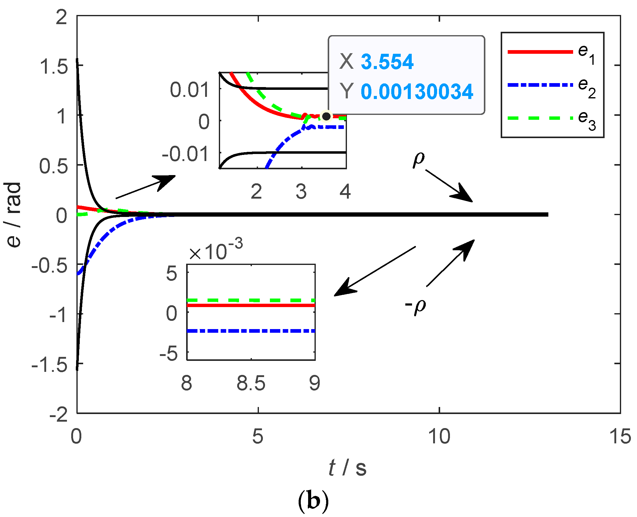
The joint tracking error curves of PPC method are given in Figure 8a, and which of SMC method are given in Figure 8b. For the convergence time, the error under the control of PPC method is stable convergence at 1.413 s and which is stable convergence under the control of SMC method at 3.554 s. For the error range, it is enveloped by the prescribed performance function under the control of PPC method while it is beyond the boundary of the same function under the control of SMC method. For the control accuracy, the PPC method is better than the SMC method. Analysis of the results shows that the PPC method can ensure that the tracking error is always within the predetermined boundaries. Therefore, the transient and steady state performance of space robot system has been improved.
Figure 4, Figure 5, Figure 6, Figure 7 and Figure 8 show that both the PPC method and SMC method can complete the on-orbit insertion operation.
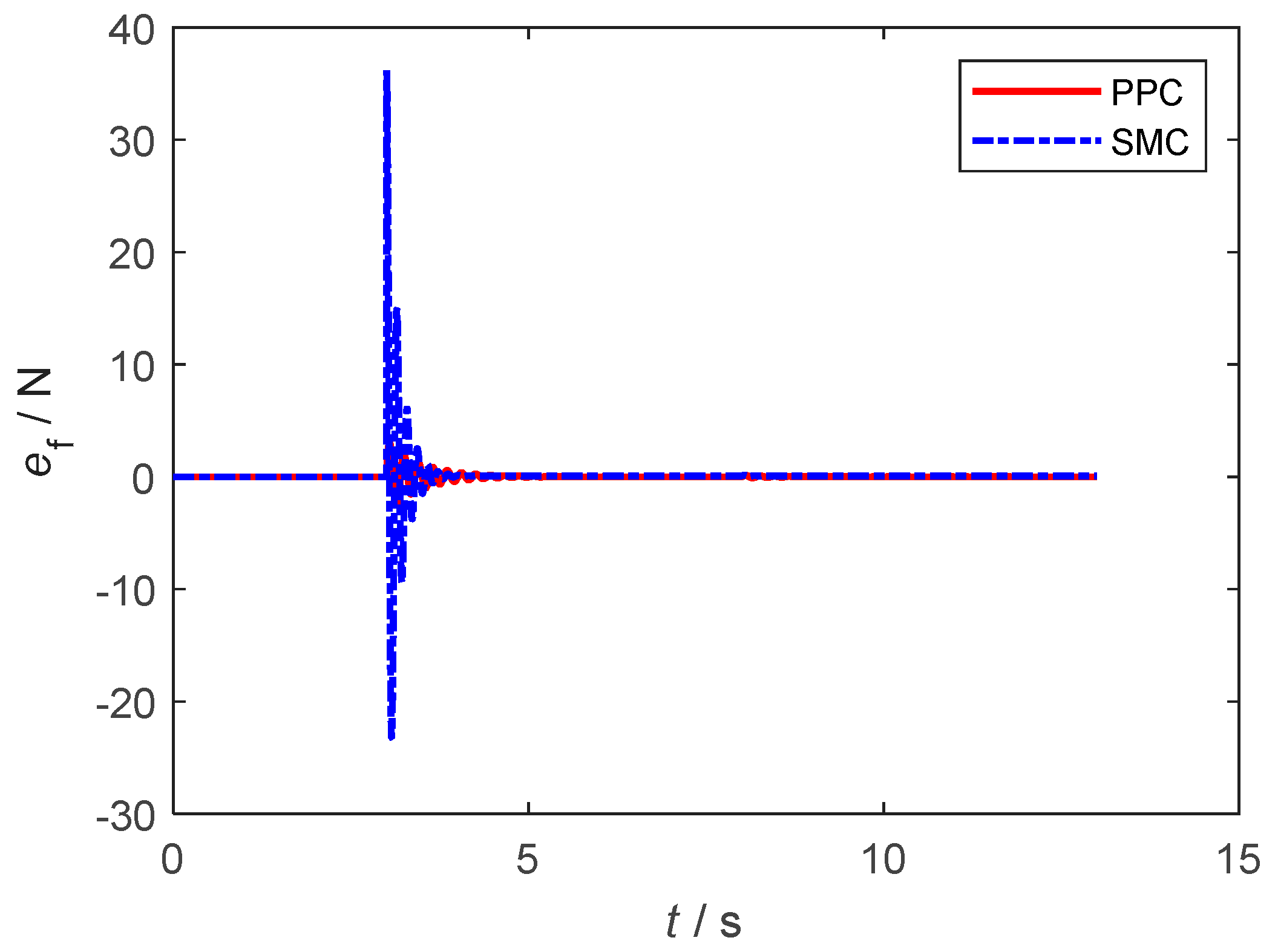
Figure 9 shows the output force of space robot end tracking error which is defined as . It is obvious that the error of PPC method is more smaller fluctuating than that of SMC method in 3~4 s, which means the insertion process of PPC method is more flexible. From the perspective of engineering practice, it is not only conducive to improve the success rate of insertion operation, but also conducive to the protection of space robot and other hardware equipment.
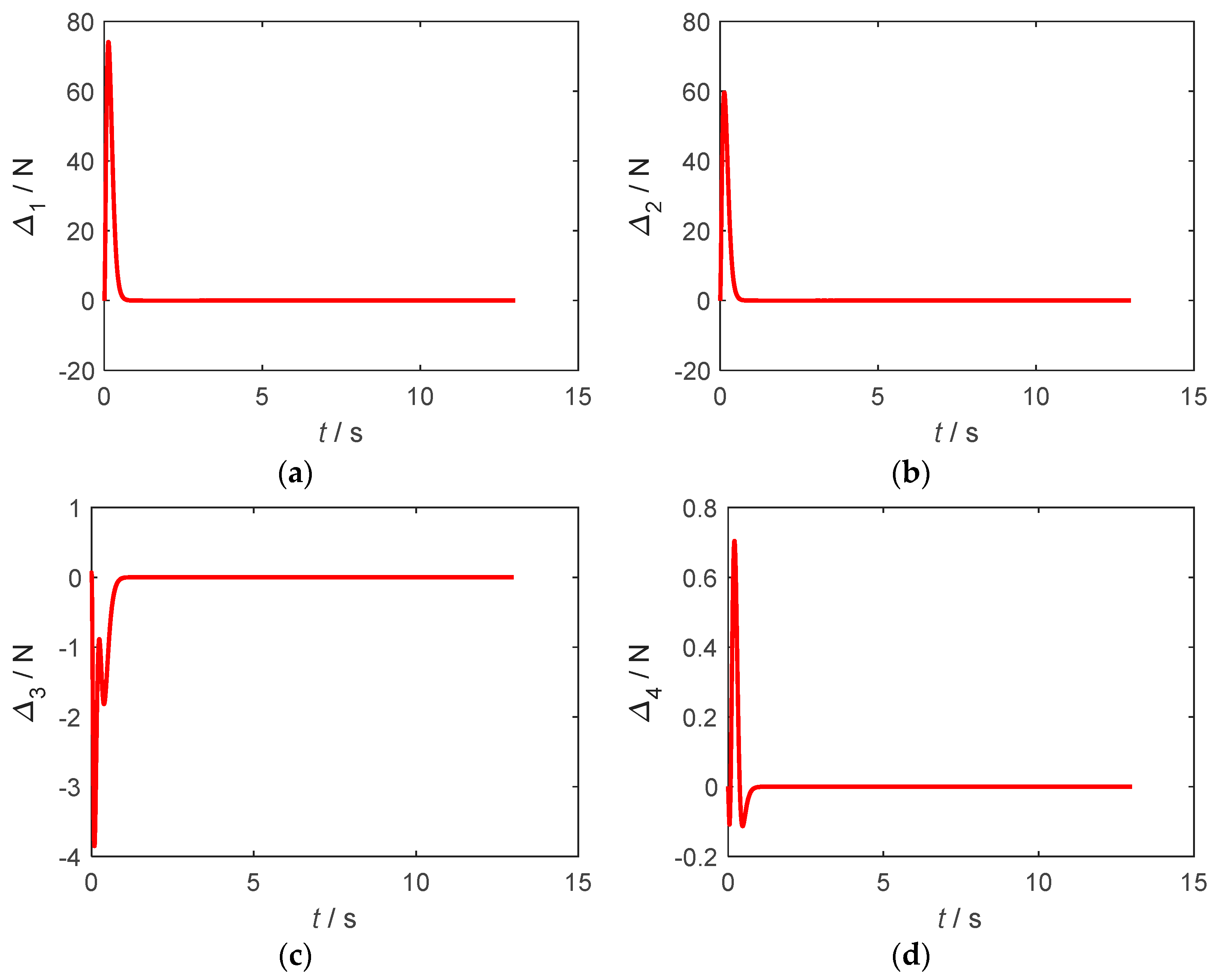
Figure 10a–d shows the unknown system dynamic estimator errors of the carrier and joints. These figures illustrated that the estimator can precisely compensate the dynamic uncertainties which consists of and . It also indicates that the robustness of space robot system is enhanced.
5.2. Details and Results of the Second Simulation Condition
Suppose that there is a sudden change of the friction happened when the insertion operation proceeding to four fifths. Other conditions of the second simulation are same as the first. The friction of second condition can be expressed as:
The control strategy is to stop the insertion and gradually increase the output force until it exceeds the friction after the sudden change happened.
The expected trajectory and output force are, respectively, designed as:
The second simulation control parameters are the same as the first and the total simulation time is 19 s. Its simulation results are shown in the following figures.
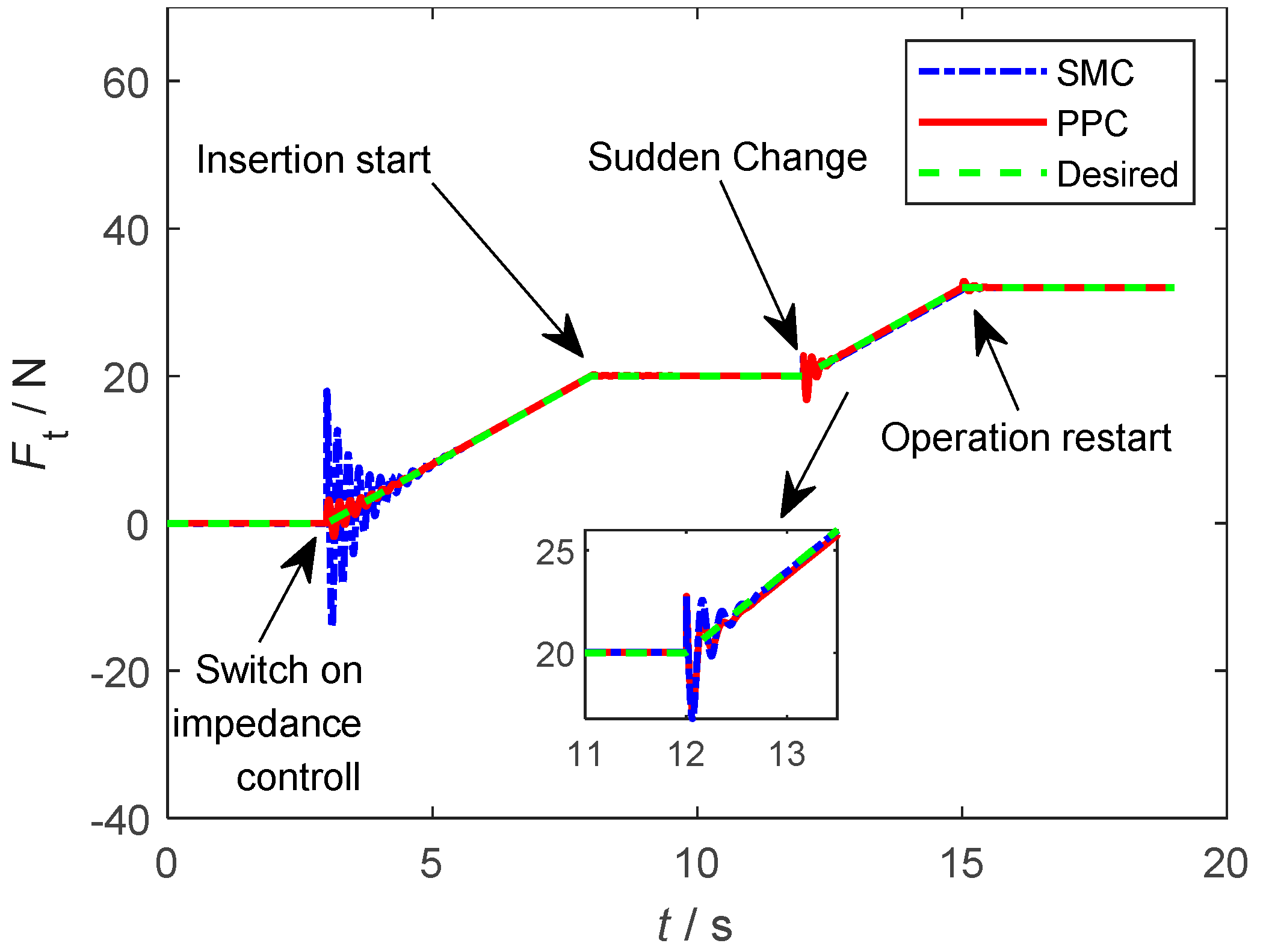
Figure 11c shows that the sudden change of friction happens at 12 s and the space robot end stop the insertion during 12–15 s. Then, the operation restart at a slower speed until the space robot end force output by impedance controller is greater the friction after sudden change. It also can be found that what expressed in Figures 13 and 14 is consistent with the above content.
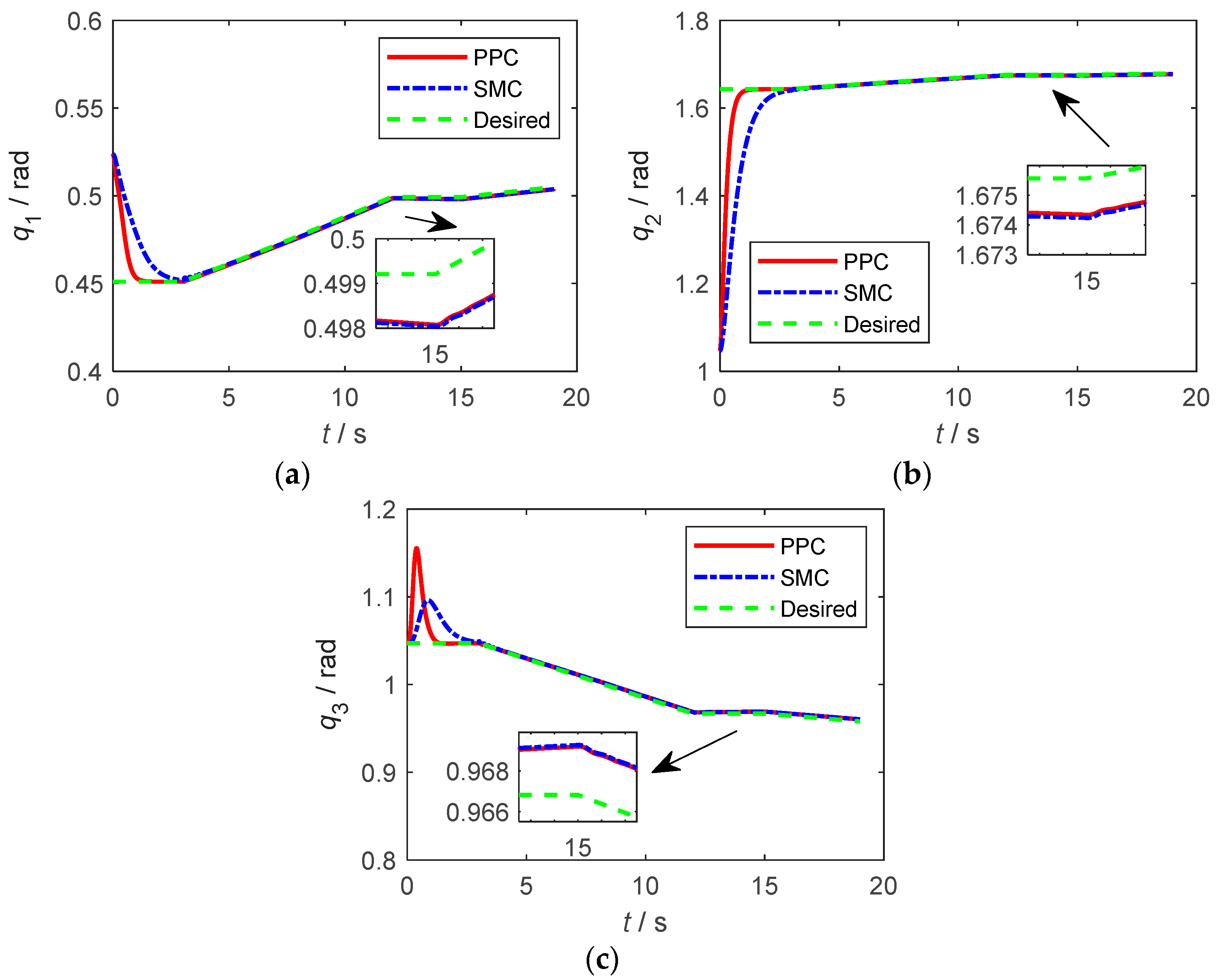
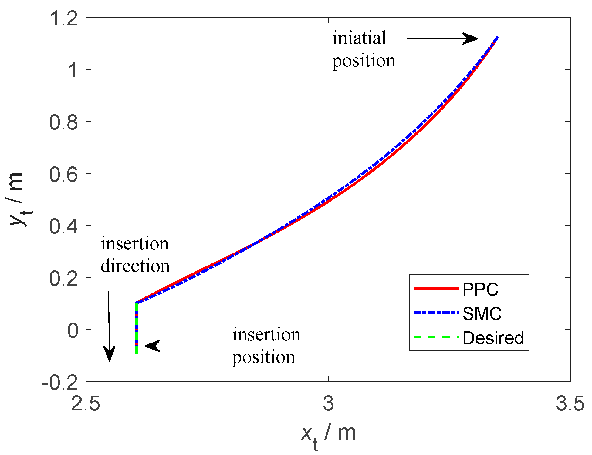
Figure 12a–c and Figure 13 are extended descriptions of the second simulation condition. That is the space robot joint trajectories and end trajectory of XY two dimensional.
Figure 12a–c show that the convergence rate is about 2 s faster than that of SMC method. In addition, the control accuracy of PPC method is better at . This is conducive to the rapid response of the space manipulator when executing the operation of inserting and extracting.
Figure 14 is the force tracking curve of space robot end. The sudden change of friction mentioned in working conditions happens at 12 s. It can be found that the vibration amplitude of end output force of PPC is much less than that of SMC in 3~5 s. This vibration is an adverse effect on the manipulator performing space tasks. The longer it lasts, the more difficult it is to adjust the attitude of the space robot in carrying out the space tasks. Thus, affecting the success rate of task execution.
The comprehensive comparison results in Section 5.1 are similar to those in Section 5.2, this shows that our proposed algorithm has faster convergence speed and smaller tracking error, and can quickly stabilize and track the output expected force in case of sudden change in the end environment.
5.3. Details and Results of the Third Simulation Condition
Suppose that the extraction operation is the inverse process of the insertion. Then, an extraction simulation condition is designed based on the first simulation condition.
The expected trajectory and output force are, respectively, designed as:
The setting of simulation parameters is consistent with that in Section 5.1 The results of extraction condition are shown in Figure 15, Figure 16, Figure 17 and Figure 18. Different from the two previous working conditions, the trajectories shown in Figure 15b,c and Figure 17 belong to the manipulator end without the replaceable instrument.
In Figure 15c, the manipulator end effector clamps the target and executes the extraction mission at 8 s. In addition, completes the extraction mission at 13 s with a setup of constant friction.
Figure 16a–c are the joint tracking curve of space robot. The extracting operation is executed at 8 s. Taking t = 8 s as the central axis, it can be found that the joint trajectories at 3~8 s and 8~13 s are symmetrical. In addition, this is consistent with the setting in the extracting work condition.
Figure 17 shows the XY two-dimensional trajectory of manipulator end without replaceable instruments. Figure 18 is the tracking curve of output force of the end.
The same conclusions can be analyzed by the extraction comparison results in Section 5.3. These results of three simulating conditions consistently illustrate that the advantages of our proposed algorithm from multiple aspects. It is worth mentioning that the transient performance of PPC controller is much better than that of SMC controller.
6. Conclusions
In this paper, the dynamics model of free-floating space robot with carrier position uncontrolled and attitude controlled is firstly established to solve the problem of on-orbit insertion and extraction of space robot. To avoid the introduction of acceleration signal, the filter operation is introduced based on the reconstruction. By using PPC method, the sliding mode controller is designed to ensure the transient and steady state performance of the system and compared with the sliding mode controller. The simulation results indicate that:
- The space robot successfully realized the operation of on-orbit insertion and extraction under the setting of simulation conditions. In addition, the vertical inserting and extracting and precise position tracking are ensured by the proposed algorithm. Therefore, the adverse effects brought out by the impact are also reduced.
- The output force of the manipulator end is tracked precisely and stably, which is good for these operations. The controlled system is robust which can adjust its output force according to the actual change of friction.
- Compared with sliding mode controller, the PPC controller has a better convergence performance and a higher control accuracy. The calculation amount of PPC controller is reduced due to the acceleration signal is avoided being introduced and its control parameters are easy to be adjusted. This would benefit to the popularization and application of this method in practical engineering scenarios.
Author Contributions
Conceptualization, D.L.; methodology, D.L. and H.A.; software, D.L. and L.C.; investigation, D.L. and H.A.; writing—original draft preparation, D.L.; writing—review and editing, D.L. and H.A.; supervision, H.A. and L.C.; funding acquisition, H.A. and L.C. All authors have read and agreed to the published version of the manuscript.
Funding
This work was supported by the National Natural Science Foundation of China (Grant No. 51741502, 51775114, 11372073), Science and Technology Project of the Education Department of Jiangxi Province (Grant No. GJJ200864), Jiangxi University of Science and Technology PhD Research Initiation Fund (Grant No. 205200100514), the Fujian Provincial High-End Equipment Manufacturing Collaborative Innovation Center (Grant No. 2021-C-275).
Informed Consent Statement
Informed consent was obtained from all subjects involved in the study.
Conflicts of Interest
The authors declare no conflict of interest.
Appendix A. System Dynamic Modeling and Motion Jacobian
In the global inertial coordinates system , the geometric position relation of each part of the space robot system with respect to the origin can be expressed as the following:
where is the position of base centroid in and are the unit vector in the direction of , respectively.
The velocity vector can be obtained by taking the first derivative of Equation (A1) with respect to time, then we have:
where are the unit velocity vector in the direction of .
According to the centroid velocity vector expression of each split body in Equation (A2), the kinetic energy expression of each split body of the space robot system can be solved as:
where indicates the kinetic energy of the base, kinetic energy of each arm, and indicates the kinetic energy of the end replaceable instrument .
The total kinetic energy of the system is the sum of the kinetic energy of each component, then we have:
Ignoring the influence of the weak gravity gradient in space, the gravitational potential energy can be simply written as:
Then the Lagrange function can be expressed as:
Combined with the second Lagrange modeling method and Equation (A6), the dynamics equation of a rigid space robot system with carrier position uncontrolled and attitude controlled can be derived as:
The kinetic equation satisfies the following:
Property A1.
, are uniformly ultimate boundedness.
where are positive constant.
Property A2.
satisfies the skew symmetry.
Assumption A1.
The external disturbances and their derivatives are bounded.
where and are positive constant.
Considering the mission design requirements, the motion Jacobian relation of the point ‘t’ on the end replaceable instrument relative to the origin in needs to be studied. When the vector is projected within the coordinate system , we have:
where indicates the length of space robot arm when being attached with end replaceable instrument .
In coordinate system , the attitude of the end replaceable instrument is in line with , then we have:
The Jacobian relation of the relative motion of the end point of the end replaceable instrument is obtained by taking the time derivative of Equation (A8), then we have:
References
- Nguyen, P.; Ravindran, R.; Carr, R.; Gossain, D.; Doetsch, K. Structural flexibility of the Shuttle remote manipulator system mechanical arm. In Proceedings of the Guidance & Control Conference, San Diego, CA, USA, 9–11 August 1982; pp. 246–256. [Google Scholar]
- Cocuzza, S.; Pretto, I.; Debei, S. Least-Squares-Based Reaction Control of Space Manipulators. J. Guid. Control Dyn. 2012, 35, 976–986. [Google Scholar] [CrossRef]
- Sands, T. Development of deterministic artificial intelligence for unmanned underwater vehicles (UUV). J. Mar. Sci. Eng. 2020, 8, 578. [Google Scholar] [CrossRef]
- Wu, J.; Wang, J.; You, Z. An overview of dynamic parameter identification of robots. Robot. Comput.-Integr. Manuf. 2010, 26, 414–419. [Google Scholar] [CrossRef]
- Liu, X.; Li, H.; Wang, J.; Cai, G. Dynamics analysis of flexible space robot with joint friction. Aerosp. Sci. Technol. 2015, 47, 164–176. [Google Scholar] [CrossRef]
- Flores-Abad, A.; Ma, O.; Pham, K.; Ulrich, S. A review of space robotics technologies for on-orbit servicing. Prog. Aerosp. Sci. 2014, 68, 1–26. [Google Scholar] [CrossRef] [Green Version]
- Antonelli, G.; Caccavale, F.; Chiacchio, P. A systematic procedure for the identification of dynamic parameters of robot manipulators. Robotica 1999, 17, 427–435. [Google Scholar] [CrossRef]
- Gautier, M. Dynamic identification of robots with power model. In Proceedings of the International Conference on Robotics and Automation, Albuquerque, NM, USA, 25 April 1997; Volume 3, pp. 1922–1927. [Google Scholar]
- Beschi, M.; Villagrossi, E.; Pedrocchi, N.; Tosatti, L.M. A general analytical procedure for robot dynamic model reduction. In Proceedings of the 2015 IEEE/RSJ International Conference on Intelligent Robots and Systems (IROS), Hamburg, Germany, 28 September–2 October 2015; pp. 4127–4132. [Google Scholar]
- Iriarte, X.; Ros, J.; Mata, V.; Aginaga, J. Determination of the symbolic base inertial parameters of planar mechanisms. Eur. J. Mech.-A/Solids 2017, 61, 82–91. [Google Scholar] [CrossRef]
- de Wit, C.C.; Olsson, H.; Astrom, K.J.; Lischinsky, P. A new model for control of systems with friction. IEEE Trans. Autom. Control 1995, 40, 419–425. [Google Scholar] [CrossRef] [Green Version]
- Cheng, J.; Chen, L. Mechanical analysis and calm control of dual-arm space robot for capturing a satellite. Lixue Xuebao Chin. J. Theor. Appl. Mech. 2016, 48, 832–842. [Google Scholar]
- Ai, H.; Chen, L. Force/position fuzzy control of space robot capturing spacecraft by dual-arm clamping. J. Harbin Eng. Univ. 2020, 41, 1847–1853. [Google Scholar]
- Fu, X.; Ai, H.; Chen, L. Repetitive learning sliding mode stabilization control for a flexible-base, flexible-link and flexible-joint space robot capturing a satellite. Appl. Sci. 2021, 11, 2076. [Google Scholar] [CrossRef]
- Ai, H.; Zhu, A.; Wang, J.; Yu, X.; Chen, L. Buffer compliance control of space robots capturing a non-cooperative spacecraft based on reinforcement learning. Appl. Sci. 2021, 11, 5783. [Google Scholar] [CrossRef]
- Liu, Y.; Yu, Z.; Liu, X.; Chen, J.; Cai, G. Active detumbling technology for noncooperative space target with energy dissipation. Adv. Space Res. 2019, 63, 1813–1823. [Google Scholar] [CrossRef]
- Han, D.; Liu, Z.; Huang, P. Capture and Detumble of a Non-cooperative Target without a Specific Gripping Point by a Dual-arm Space Robot. Adv. Space Res. 2022, 69, 3770–3784. [Google Scholar] [CrossRef]
- Dai, H.; Cao, X.; Jing, X.; Wang, X.; Yue, X. Bio-inspired anti-impact manipulator for capturing non-cooperative spacecraft: Theory and experiment. Mech. Syst. Signal Process. 2020, 142, 106785. [Google Scholar] [CrossRef]
- Yan, W.; Liu, Y.; Lan, Q.; Zhang, T.; Tu, H. Trajectory planning and low-chattering fixed-time nonsingular terminal sliding mode control for a dual-arm free-floating space robot. Robotica 2022, 40, 625–645. [Google Scholar] [CrossRef]
- Seraji, H.; Colbaugh, R. Force tracking in impedance control. In Proceedings of the IEEE International Conference on Robotics and Automation, Atlanta, GA, USA, 2–6 May 1993; Volume 2, pp. 499–506. [Google Scholar]
- Lange, F.; Bertleff, W.; Suppa, M. Force and trajectory control of industrial robots in stiff contact. In Proceedings of the 2013 IEEE International Conference on Robotics and Automation, Karlsruhe, Germany, 6–10 May 2013; pp. 2927–2934. [Google Scholar]
- Roveda, L.; Iannacci, N.; Vicentini, F.; Pedrocchi, N.; Braghin, F.; Tosatti, L.M. Optimal Impedance Force-Tracking Control Design with Impact Formulation for Interaction Tasks. IEEE Robot. Autom. Lett. 2016, 1, 130–136. [Google Scholar] [CrossRef]
- Kizir, S.; Elşavi, A. Position-Based Fractional-Order Impedance Control of a 2 DOF Serial Manipulator. Robotica 2021, 39, 1560–1574. [Google Scholar] [CrossRef]
- Izadbakhsh, A.; Khorashadizadeh, S. Polynomial-Based Robust Adaptive Impedance Control of Electrically Driven Robots. Robotica 2021, 39, 1181–1201. [Google Scholar] [CrossRef]
- Polverini, M.P.; Zanchettin, A.M.; Castello, S.; Rocco, P. Sensorless and constraint-based peg-in-hole task execution with a dual-arm robot. In Proceedings of the 2016 IEEE International Conference on Robotics and Automation (ICRA), Stockholm, Sweden, 16–21 May 2016; pp. 415–420. [Google Scholar]
- Yao, Y.; Ding, L.; Ma, R.; Wang, Y. Robust Control for a Cable-driven Aerial Manipulator with Joint Flexibility in Joint Space. Control Decis. 2021, 1893, online ahead of print. [Google Scholar]
- Jia, Q.; Yuan, B.; Chen, G.; Fu, Y. Adaptive fuzzy terminal sliding mode control for the free-floating space manipulator with free-swinging joint failure. Chin. J. Aeronaut. 2021, 34, 178–198. [Google Scholar] [CrossRef]
- Zhan, B.; Jin, M.; Yang, G.; Zhang, C. A novel strategy for space manipulator detumbling a non-cooperative target with collision avoidance. Adv. Space Res. 2020, 66, 785–799. [Google Scholar] [CrossRef]
- Yang, Y. Analytic LQR design for spacecraft control system based on quaternion model. J. Aerosp. Eng. 2011, 25, 448–453. [Google Scholar] [CrossRef]
- Mehrzad, S.; Mehdi, K.; Arun, K. Dynamic analysis and trajectory tracking of a tethered space robot. Acta Astronaut. 2016, 128, 335–342. [Google Scholar]
- Li, Y.; Hao, X.; She, Y.; Li, S.; Yu, M. Constrained motion planning of free-float dual-arm space manipulator via deep reinforcement learning. Aerosp. Sci. Technol. 2021, 109, 106446. [Google Scholar] [CrossRef]
- Bechlioulis, C.P.; Rovithakis, G.A. Robust adaptive control of feedback linearizable MIMO nonlinear systems with prescribed performance. IEEE Trans. Autom. Control 2008, 53, 2090–2099. [Google Scholar] [CrossRef]
- Wei, C.; Luo, J.; Ma, C.; Dai, H.; Yua, J. Event-triggered neuroadaptive control for postcapture spacecraft with ultralow-frequency actuator updates. Neurocomputing 2018, 315, 310–321. [Google Scholar] [CrossRef]
- Yao, Q. Adaptive trajectory tracking control of a free-flying space manipulator with guaranteed prescribed performance and actuator saturation. Acta Astronaut. 2021, 185, 283–298. [Google Scholar] [CrossRef]
- Li, X.; Luo, X.; Wang, J.; Guan, X. Finite-time consensus of nonlinear multi-agent system with prescribed performance. Nonlinear Dyn. 2018, 91, 2397–2409. [Google Scholar] [CrossRef]
Figure 1.
Three-link single-arm rigid space robot structure diagram.

Figure 2.
The control structure of space robot system.

Figure 3.
The space robot operation of insertion and extraction diagram.

Figure 4.
Space robot end trajectory tracking curve of on-orbit insertion operation. (a) The carrier attitude, (b) The X-direction position, (c) The Y-direction position, (d) The space robot end attitude.
Figure 4.
Space robot end trajectory tracking curve of on-orbit insertion operation. (a) The carrier attitude, (b) The X-direction position, (c) The Y-direction position, (d) The space robot end attitude.

Figure 5.
Joint trajectory tracking curve of on-orbit insertion operation. (a) The joint , (b) The joint , (c) The joint .
Figure 5.
Joint trajectory tracking curve of on-orbit insertion operation. (a) The joint , (b) The joint , (c) The joint .

Figure 6.
Space robot end X&Y-direction trajectory tracking curve of on-orbit insertion operation.

Figure 7.
Output force of space robot end tracking curve of on-orbit insertion operation.

Figure 8.
The joint tracking error curve of space robot end on-orbit insertion operation. (a) PPC. (b) SMC.
Figure 8.
The joint tracking error curve of space robot end on-orbit insertion operation. (a) PPC. (b) SMC.


Figure 9.
Force tracking error curve of space robot end on-orbit insertion operation.

Figure 10.
The tracking error of unknown system dynamic estimator. (a) The carrier . (b) The joint . (c) The joint . (d) The joint .
Figure 10.
The tracking error of unknown system dynamic estimator. (a) The carrier . (b) The joint . (c) The joint . (d) The joint .

Figure 11.
Space robot end trajectory tracking curve of on-orbit insertion operation. (a) The carrier attitude. (b) The X-direction position. (c) The Y-direction position. (d) The space robot end attitude.
Figure 11.
Space robot end trajectory tracking curve of on-orbit insertion operation. (a) The carrier attitude. (b) The X-direction position. (c) The Y-direction position. (d) The space robot end attitude.

Figure 12.
Joint trajectory tracking curve of on-orbit insertion operation. (a) The joint . (b) The joint . (c) The joint .
Figure 12.
Joint trajectory tracking curve of on-orbit insertion operation. (a) The joint . (b) The joint . (c) The joint .

Figure 13.
Space robot end X&Y-direction trajectory tracking curve of on-orbit insertion operation with friction change.
Figure 13.
Space robot end X&Y-direction trajectory tracking curve of on-orbit insertion operation with friction change.

Figure 14.
Output force of space robot end tracking curve of on-orbit insertion operation with friction change.
Figure 14.
Output force of space robot end tracking curve of on-orbit insertion operation with friction change.

Figure 15.
Space robot end trajectory tracking curve of on-orbit extraction operation. (a) The carrier attitude. (b) The X-direction position. (c) The Y-direction position. (d) The space robot end attitude.
Figure 15.
Space robot end trajectory tracking curve of on-orbit extraction operation. (a) The carrier attitude. (b) The X-direction position. (c) The Y-direction position. (d) The space robot end attitude.

Figure 16.
Joint trajectory tracking curve of on-orbit extraction operation. (a) The joint . (b) The joint . (c)The joint .
Figure 16.
Joint trajectory tracking curve of on-orbit extraction operation. (a) The joint . (b) The joint . (c)The joint .


Figure 17.
Space robot end X&Y-direction trajectory tracking curve of on-orbit extraction operation.
Figure 17.
Space robot end X&Y-direction trajectory tracking curve of on-orbit extraction operation.

Figure 18.
Output force of space robot end tracking curve of on-orbit extraction operation.

Publisher’s Note: MDPI stays neutral with regard to jurisdictional claims in published maps and institutional affiliations. |
© 2022 by the authors. Licensee MDPI, Basel, Switzerland. This article is an open access article distributed under the terms and conditions of the Creative Commons Attribution (CC BY) license (https://creativecommons.org/licenses/by/4.0/).
Share and Cite
MDPI and ACS Style
Liu, D.; Ai, H.; Chen, L. Impedance Control of Space Robot On-Orbit Insertion and Extraction Based on Prescribed Performance Method. Appl. Sci. 2022, 12, 5147. https://0-doi-org.brum.beds.ac.uk/10.3390/app12105147
AMA Style
Liu D, Ai H, Chen L. Impedance Control of Space Robot On-Orbit Insertion and Extraction Based on Prescribed Performance Method. Applied Sciences. 2022; 12(10):5147. https://0-doi-org.brum.beds.ac.uk/10.3390/app12105147
Chicago/Turabian StyleLiu, Dongbo, Haiping Ai, and Li Chen. 2022. "Impedance Control of Space Robot On-Orbit Insertion and Extraction Based on Prescribed Performance Method" Applied Sciences 12, no. 10: 5147. https://0-doi-org.brum.beds.ac.uk/10.3390/app12105147
Note that from the first issue of 2016, this journal uses article numbers instead of page numbers. See further details here.