
An End-to-End Atrous Spatial Pyramid Pooling and Skip-Connections Generative Adversarial Segmentation Network for Building Extraction from High-Resolution Aerial Images


Abstract
:1. Introduction
- (1)
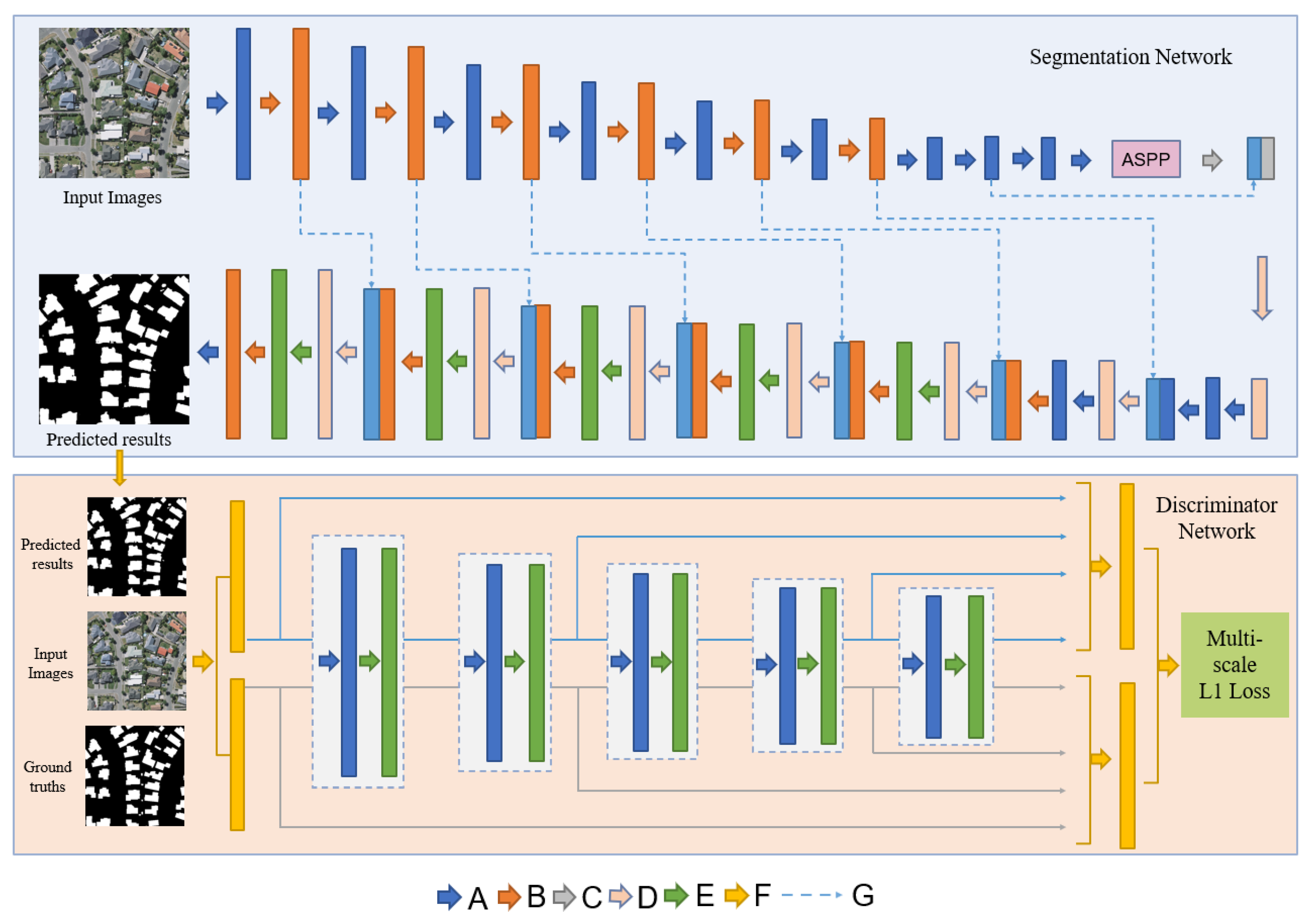
- ASGASN implements automatic and efficient building segmentation based on GAN. In this algorithm, the segmentation network provides the class-false a priori knowledge for the training of the discriminator network, and the discriminator network corrects the learning of the segmentation network through training to make the classification results more closely match the a posteriori knowledge.
- (2)
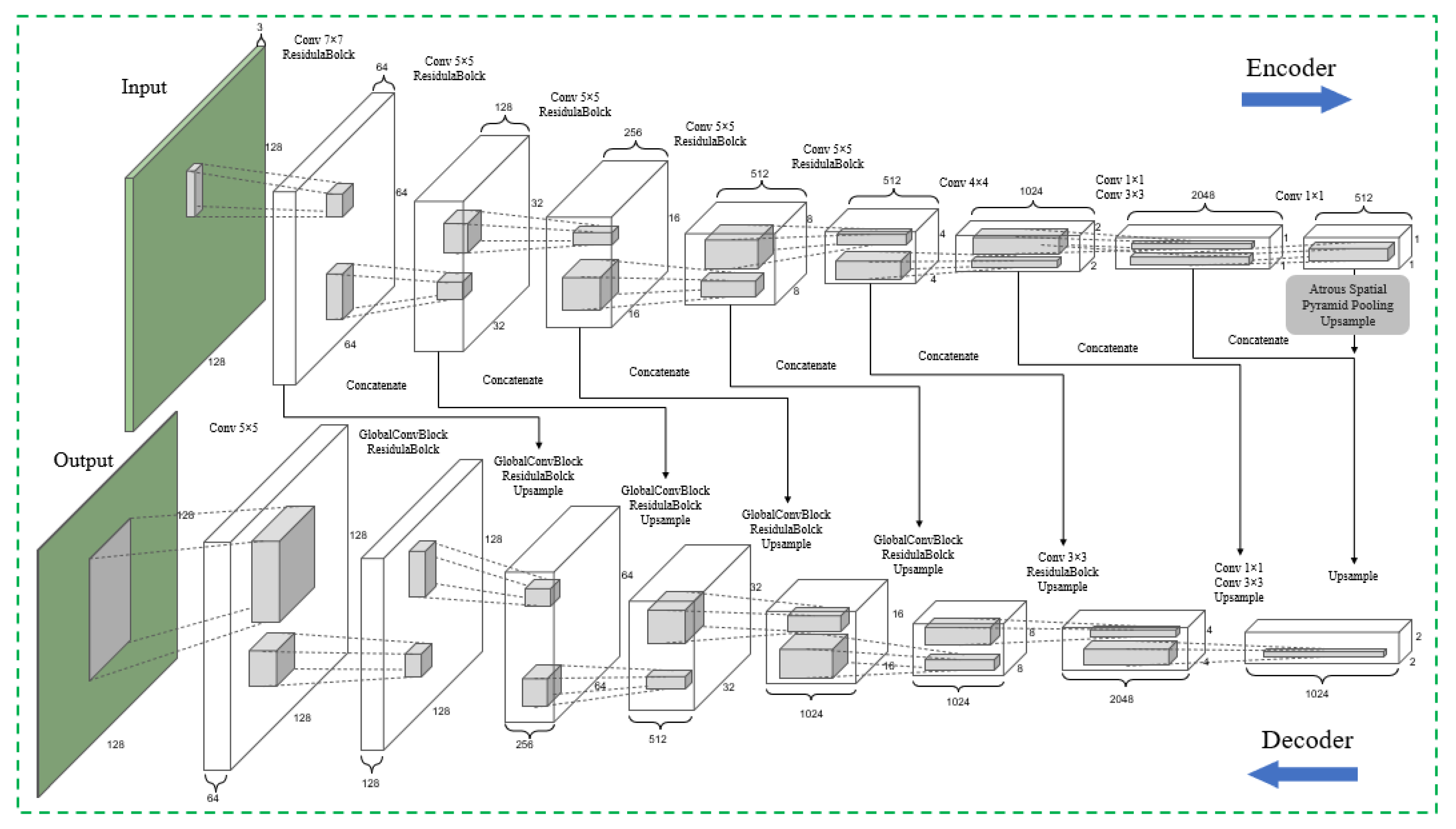
- The ASGASN architecture, into which ASPP and skip connections are embedded, allows features to be extracted from multiple spatial scales and improves segmentation accuracy by fusing multiscale information. The global convolutional block is also added to make a tight connection between the feature map and the pixel-by-pixel classifier.
- (3)
- The segmentation and discriminator network are trained alternately by multiscale L1 loss and multiple cross entropy losses, which finally make the best performance of ASGASN. We conduct relevant experiments on both the WHU building dataset [38] and the Chinese typical city building dataset [39] to verify the advancedness of the present network.
2. Methods
2.1. Proposed Network ASGASN
2.2. Segmentation Network
2.2.1. Subsubsection Atrous Spatial Pyramid Pooling
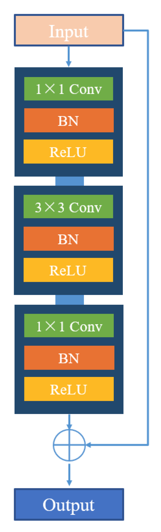
2.2.2. Residual Block
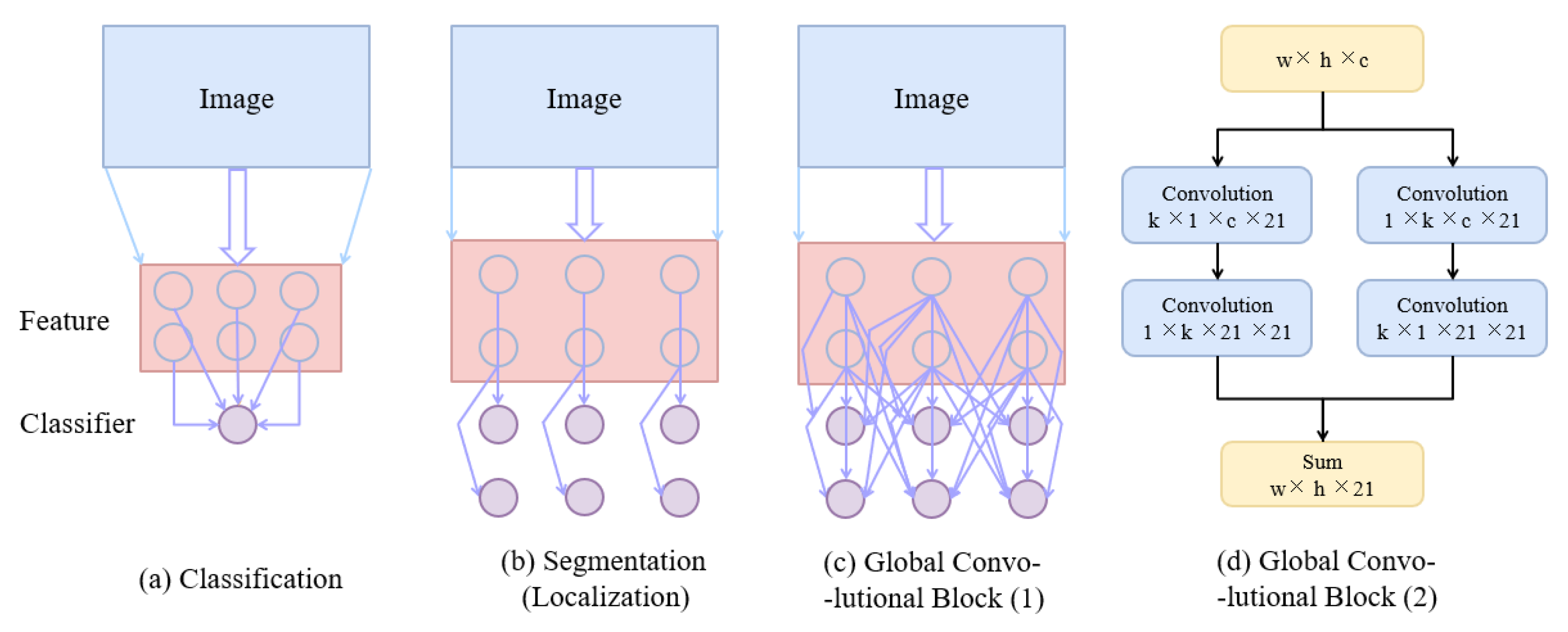
2.2.3. Global Convolutional Block
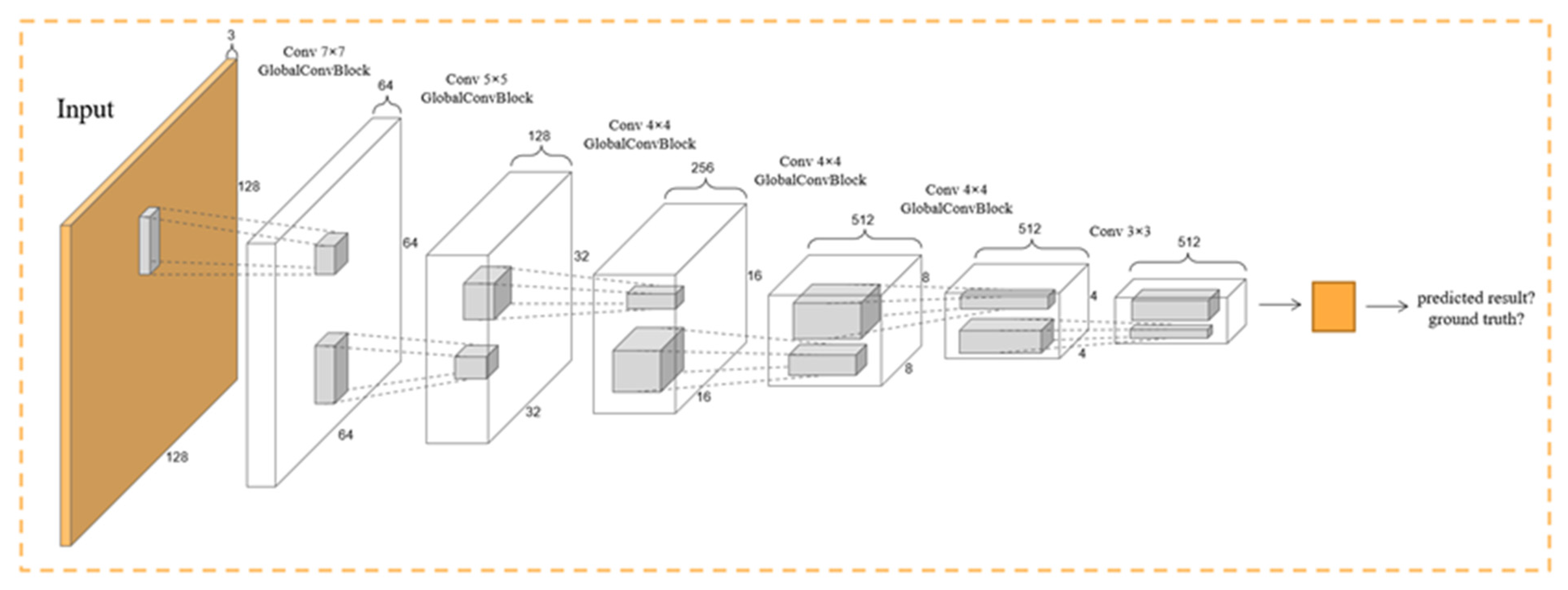
2.3. Discriminator Network
2.4. Loss Function
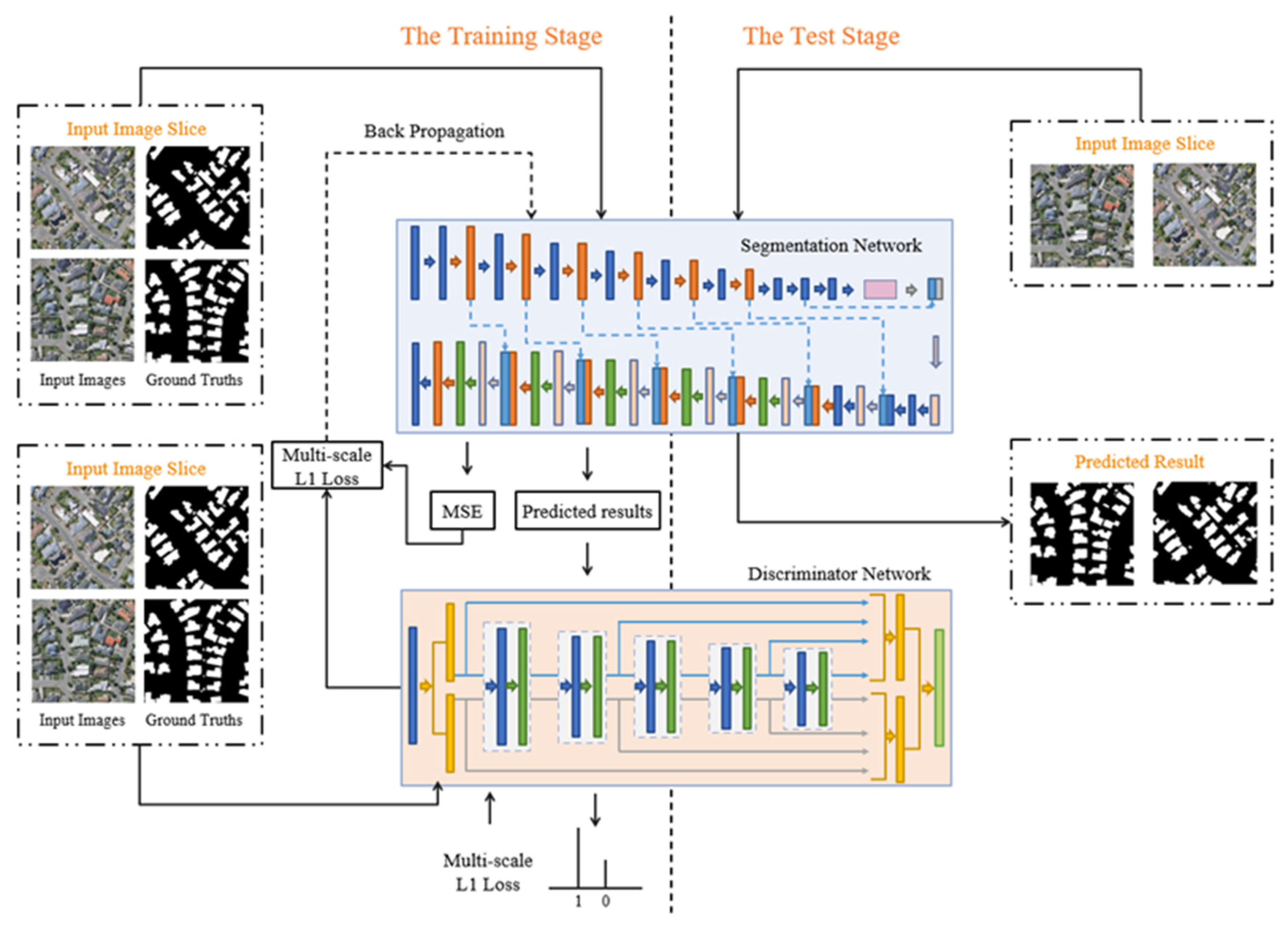
2.5. Flowchart
2.6. Pixel Analysis
3. Experiment Dataset and Evaluation
3.1. Experiment Data
3.2. Data Processing
3.3. Experiment Settings
3.4. Evaluation Metrics
- OA refers to the proportion of correctly predicted building and background pixels to all pixels in the image:
- 2
- Recall refers to the proportion of correctly predicted building pixels in the image to the true value pixels in the building area:
- 3
- Precision refers to proportion of correctly predicted building pixels to all predicted building pixels in the image:
- 4
- F1-score represents the weighted average of OA and Precision:
- 5
- IoU, which can describe segment-level accuracy:
3.5. Model Comparisons
4. Results
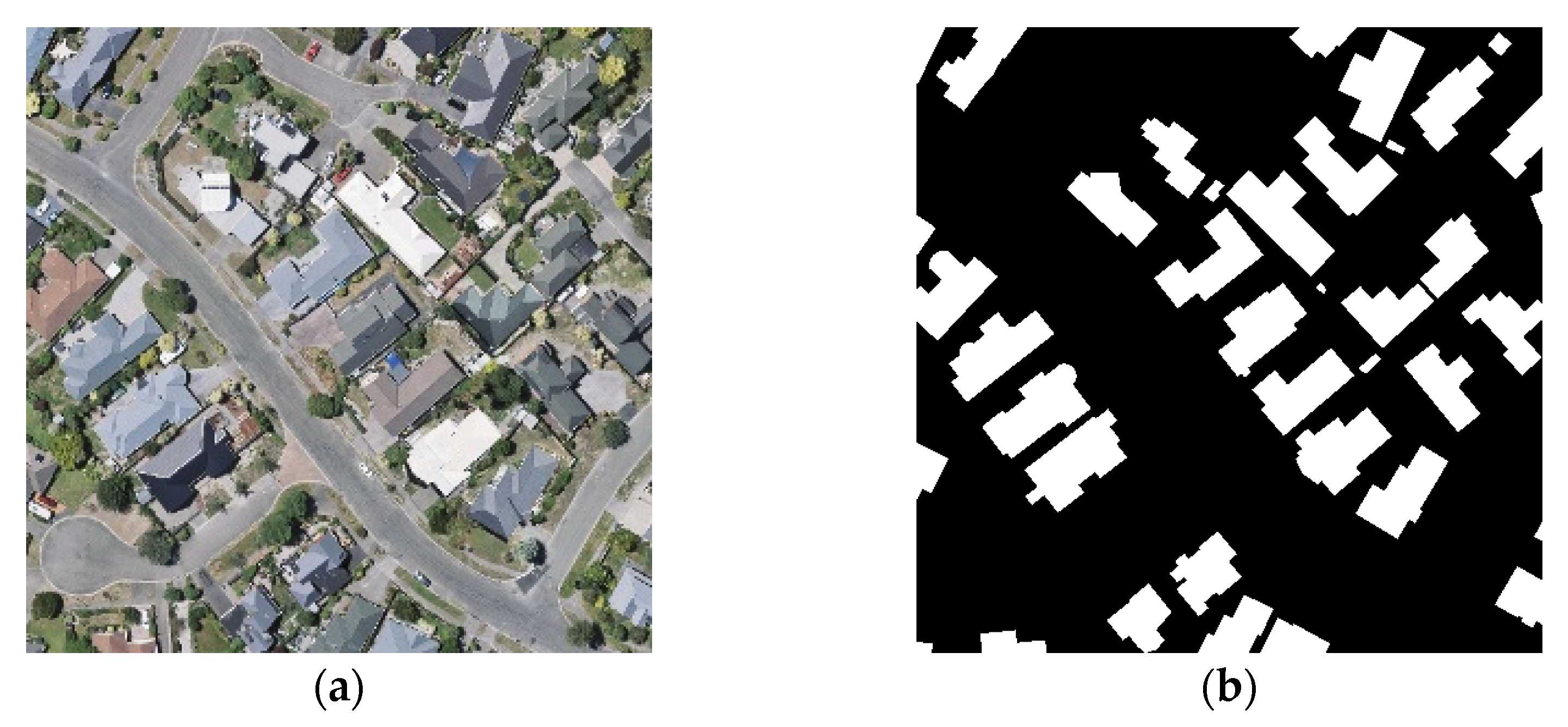
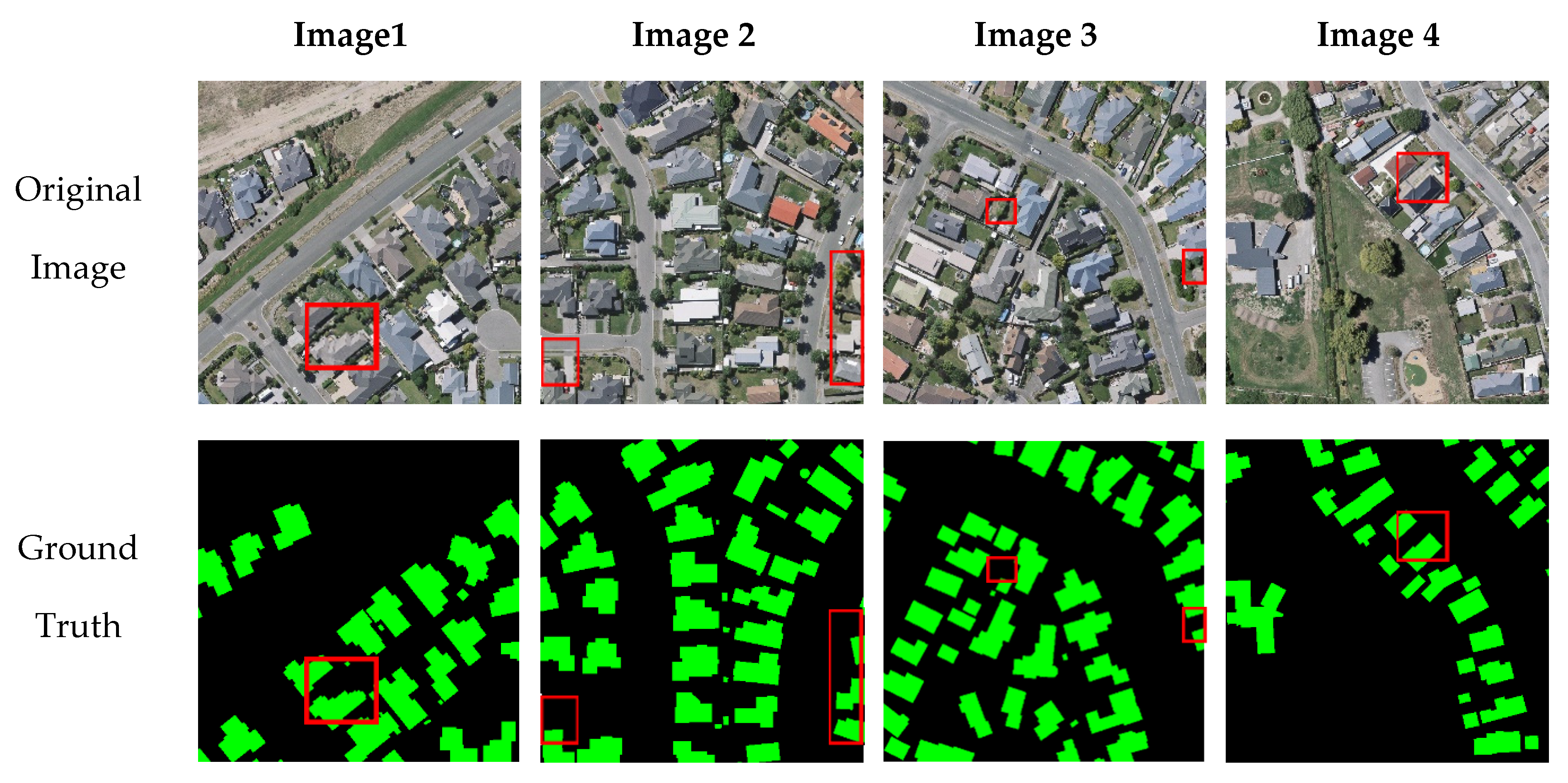
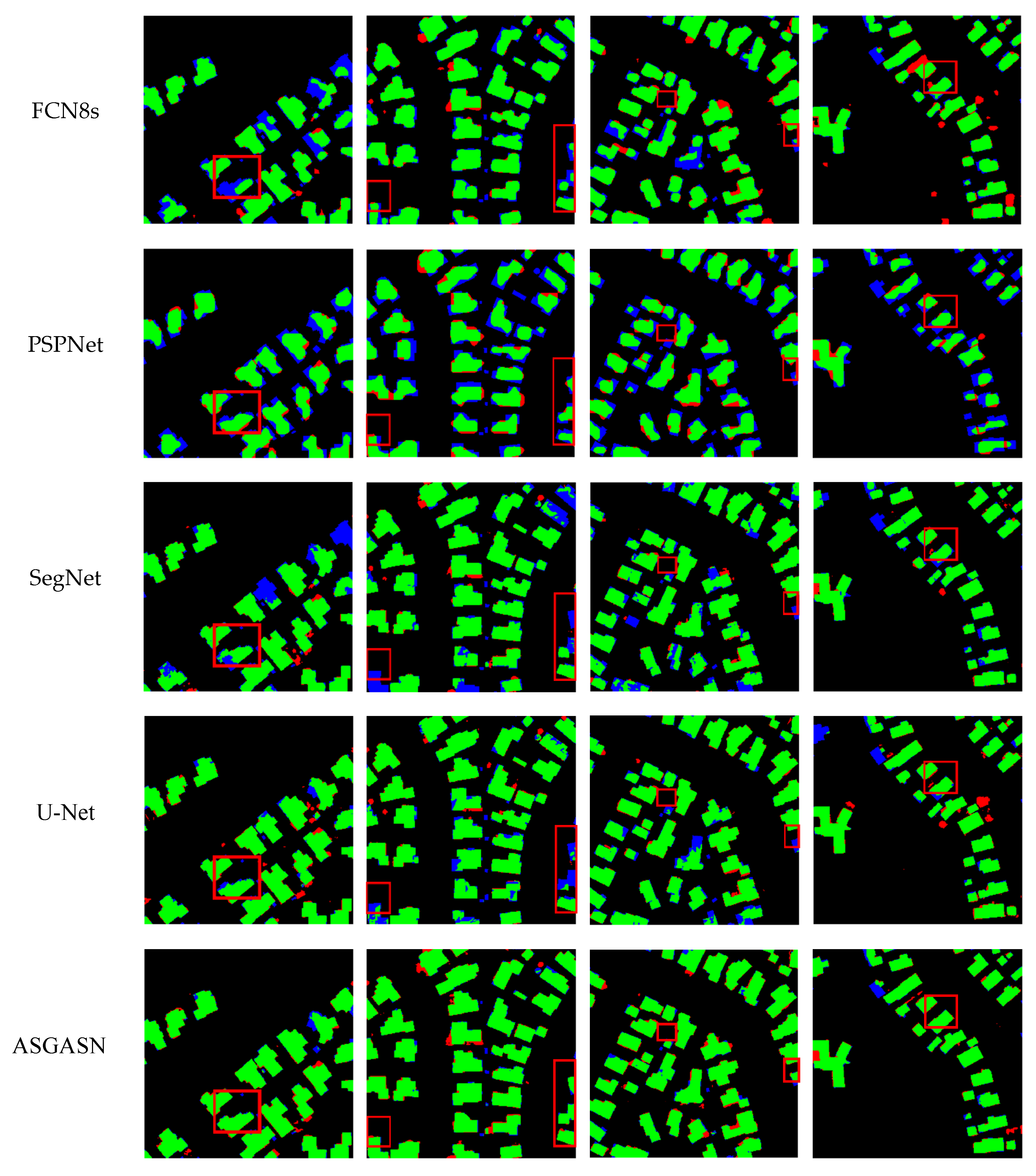
4.1. Experimental Results on the WHU Dataset
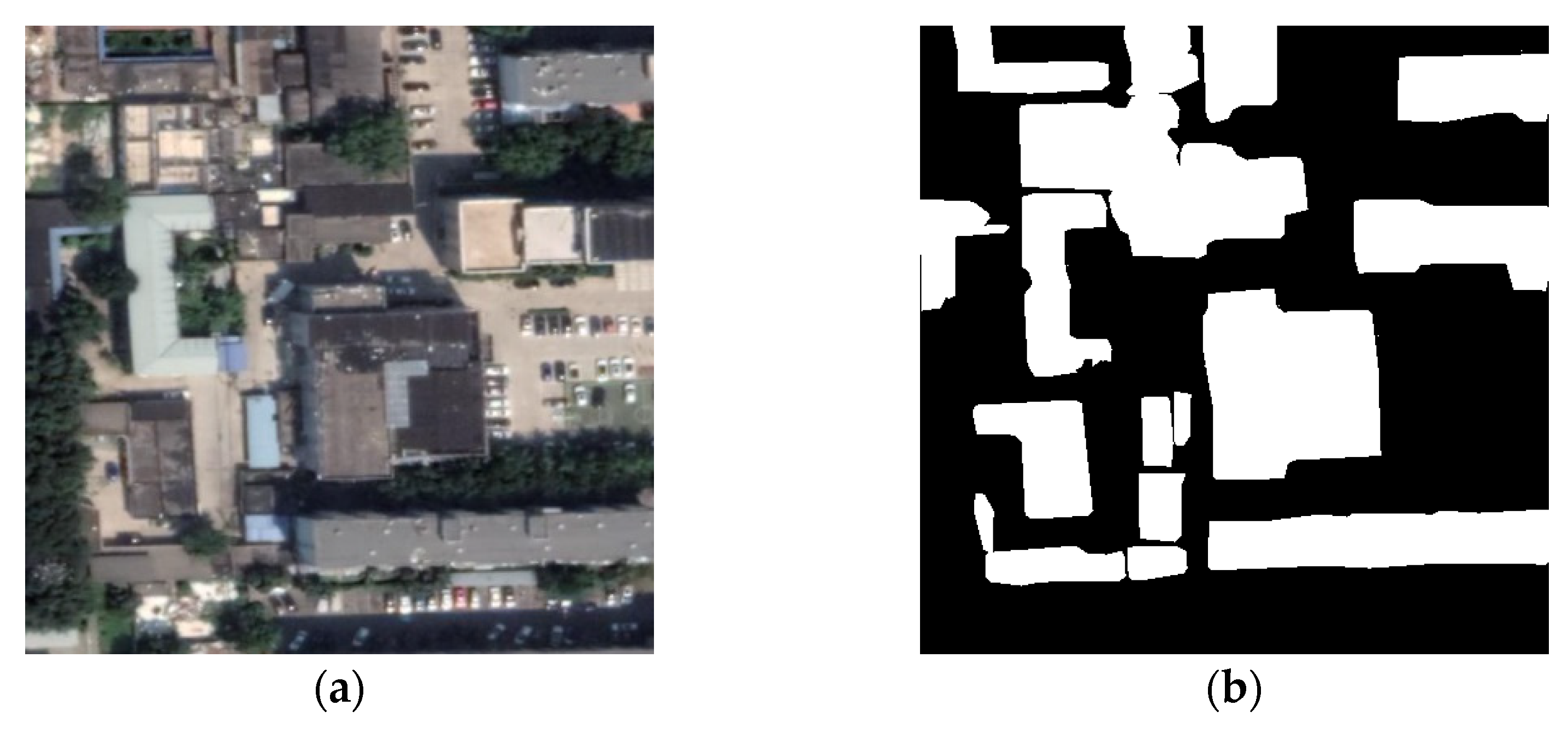
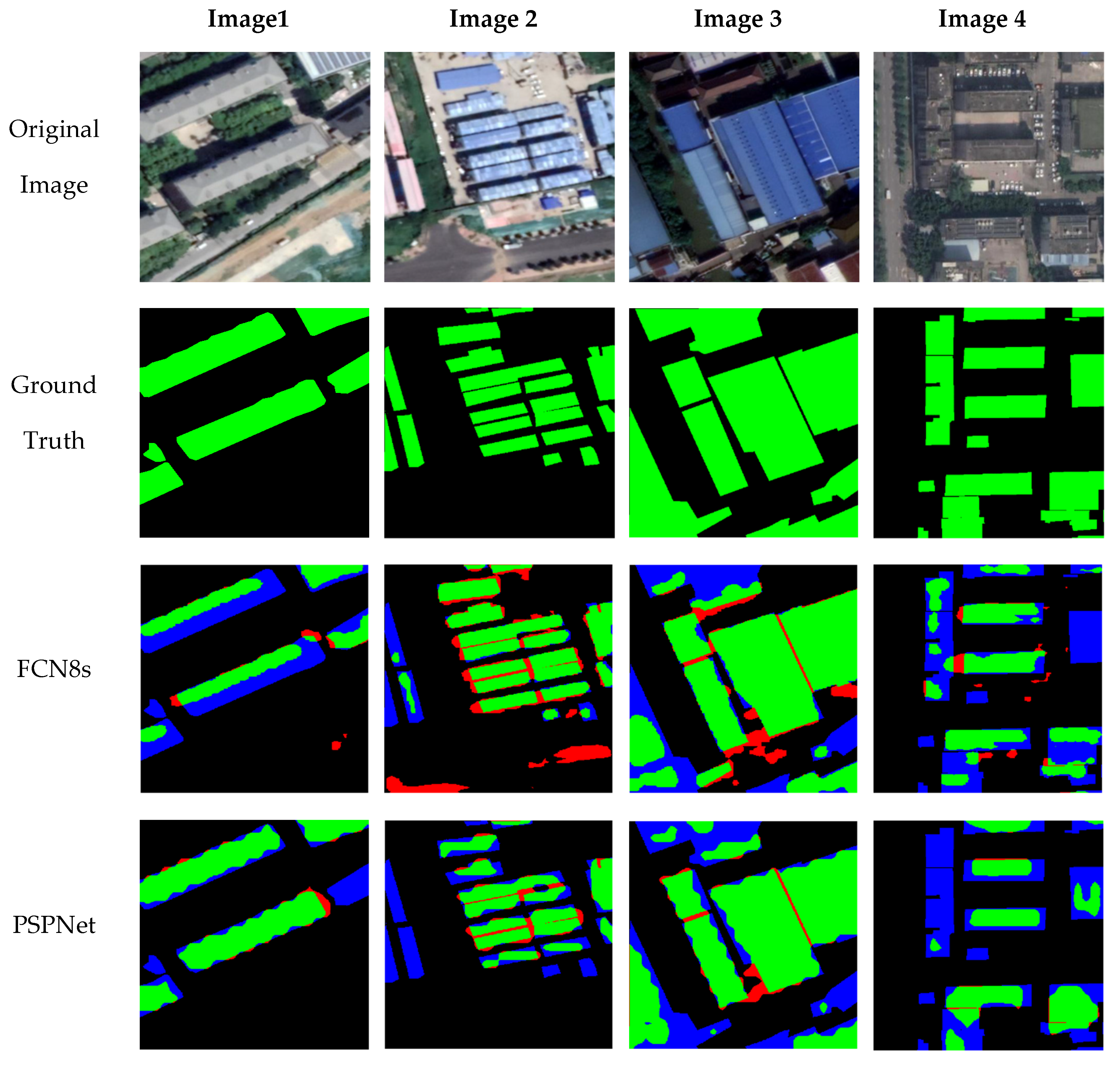
4.2. Experimental Results on the CHN Dataset
5. Discussion
5.1. About the Proposed ASGASN Model
5.2. Limitations
6. Conclusions
- (1)
- ASGASN using the adversarial training strategy can pay more attention to the relationship between pixels, improve the continuity of segmentation results, and make the extracted building boundaries clearer.
- (2)
- ASGASN introduces depth-separable convolution and global convolution to im-prove the classification and localization accuracy of the model, and uses ASPP to improve the model’s ability to perceive buildings at different scales. These measures allow the network to obtain building extraction results that are closer to the ground truth.
- (3)
- The wide applicability of ASGASN for remote sensing images is greatly improved compared with other networks. The building extraction results on the WHU dataset show that ASGASN can get better extraction results for different types of buildings. Additionally, in the quantitative evaluation metrics of both datasets, the method in this paper achieves better score performance.
Author Contributions
Funding
Institutional Review Board Statement
Informed Consent Statement
Data Availability Statement
Acknowledgments
Conflicts of Interest
References
- He, H.; Yang, D.; Wang, S.; Wang, S.; Li, Y. Road Extraction by Using Atrous Spatial Pyramid Pooling Integrated Encoder-Decoder Network and Structural Similarity Loss. Remote Sens. 2019, 11, 1015. [Google Scholar] [CrossRef] [Green Version]
- Liu, Y.; Gross, L.; Li, Z.; Li, X.; Fan, X.; Qi, W. Automatic Building Extraction on High-Resolution Remote Sensing Imagery Using Deep Convolutional Encoder-Decoder with Spatial Pyramid Pooling. IEEE Access 2019, 7, 128774–128786. [Google Scholar] [CrossRef]
- Boonpook, W.; Tan, Y.; Ye, Y.; Torteeka, P.; Torsri, K.; Dong, S. A Deep Learning Approach on Building Detection from Unmanned Aerial Vehicle-Based Images in Riverbank Monitoring. Sensors 2018, 18, 3921. [Google Scholar] [CrossRef] [Green Version]
- Liu, Y.; Zhou, J.; Qi, W.; Li, X.; Gross, L.; Shao, Q.; Zhao, Z.; Ni, L.; Fan, X.; Li, Z. ARC-Net: An Efficient Network for Building Extraction from High-Resolution Aerial Images. IEEE Access 2020, 8, 154997–155010. [Google Scholar] [CrossRef]
- Xing, H.; Zhu, L.; Hou, D.; Zhang, T. Integrating Change Magnitude Maps of Spectrally Enhanced Multi-Features for Land Cover Change Detection. Int. J. Remote Sens. 2021, 42, 4284–4308. [Google Scholar] [CrossRef]
- Cleve, C.; Kelly, M.; Kearns, F.R.; Moritz, M. Classification of the Wildland–Urban Interface: A Comparison of Pixel-and Object-Based Classifications Using High-Resolution Aerial Photography. Comput. Environ. Urban Syst. 2008, 32, 317–326. [Google Scholar] [CrossRef]
- Wang, J.; Yang, X.; Qin, X.; Ye, X.; Qin, Q. An Efficient Approach for Automatic Rectangular Building Extraction from Very High Resolution Optical Satellite Imagery. IEEE Geosci. Remote Sens. Lett. 2014, 12, 487–491. [Google Scholar] [CrossRef]
- Dalal, N.; Triggs, B. Histograms of Oriented Gradients for Human Detection. In Proceedings of the 2005 IEEE Computer Society Conference on Computer Vision and Pattern Recognition (CVPR’05), San Diego, CA, USA, 20–25 June 2005; Volume 1, pp. 886–893. [Google Scholar]
- Clausi, D.A. An Analysis of Co-Occurrence Texture Statistics as a Function of Grey Level Quantization. Can. J. Remote Sens. 2002, 28, 45–62. [Google Scholar] [CrossRef]
- Xing, H.; Zhu, L.; Feng, Y.; Wang, W.; Hou, D.; Meng, F.; Ni, Y. An Adaptive Change Threshold Selection Method Based on Land Cover Posterior Probability and Spatial Neighborhood Information. IEEE J. Sel. Top. Appl. Earth Obs. Remote Sens. 2021, 14, 11608–11621. [Google Scholar] [CrossRef]
- Kim, T.; Lee, T.-Y.; Lim, Y.J.; Kim, K.-O. The Use of Voting Strategy for Building Extraction from High Resolution Satellite Images. In Proceedings of the 2005 IEEE International Geoscience and Remote Sensing Symposium, IGARSS’05, Seoul, Korea, 29 July 2005; Volume 2, pp. 1269–1272. [Google Scholar]
- Shrivastava, N.; Kumar Rai, P. Automatic Building Extraction Based on Multiresolution Segmentation Using Remote Sensing Data. Geogr. Pol. 2015, 88, 407–421. [Google Scholar] [CrossRef] [Green Version]
- Karantzalos, K.; Paragios, N. Recognition-Driven Two-Dimensional Competing Priors toward Automatic and Accurate Building Detection. IEEE Trans. Geosci. Remote Sens. 2008, 47, 133–144. [Google Scholar] [CrossRef]
- Aytekin, Ö.; Zöngür, U.; Halici, U. Texture-Based Airport Runway Detection. IEEE Geosci. Remote Sens. Lett. 2012, 10, 471–475. [Google Scholar] [CrossRef]
- Inglada, J. Automatic Recognition of Man-Made Objects in High Resolution Optical Remote Sensing Images by SVM Classification of Geometric Image Features. ISPRS J. Photogramm. Remote Sens. 2007, 62, 236–248. [Google Scholar] [CrossRef]
- Désir, C.; Bernard, S.; Petitjean, C.; Heutte, L. One Class Random Forests. Pattern Recognit. 2013, 46, 3490–3506. [Google Scholar] [CrossRef] [Green Version]
- Guo, J.; Pan, Z.; Lei, B.; Ding, C. Automatic Color Correction for Multisource Remote Sensing Images with Wasserstein CNN. Remote Sens. 2017, 9, 483. [Google Scholar] [CrossRef] [Green Version]
- LeCun, Y.; Bottou, L.; Bengio, Y.; Haffner, P. Gradient-Based Learning Applied to Document Recognition. Proc. IEEE 1998, 86, 2278–2324. [Google Scholar] [CrossRef] [Green Version]
- Krizhevsky, A.; Sutskever, I.; Hinton, G.E. Imagenet Classification with Deep Convolutional Neural Networks. Adv. Neural Inf. Process. Syst. 2012, 25, 84–90. [Google Scholar] [CrossRef]
- Simonyan, K.; Zisserman, A. Very Deep Convolutional Networks for Large-Scale Image Recognition. arXiv 2014, arXiv:1409.1556. [Google Scholar]
- Szegedy, C.; Liu, W.; Jia, Y.; Sermanet, P.; Reed, S.; Anguelov, D.; Erhan, D.; Vanhoucke, V.; Rabinovich, A. Going Deeper with Convolutions. In Proceedings of the IEEE Conference on Computer Vision and Pattern Recognition, Boston, MA, USA, 8–10 June 2015; pp. 1–9. [Google Scholar]
- Szegedy, C.; Vanhoucke, V.; Ioffe, S.; Shlens, J.; Wojna, Z. Rethinking the Inception Architecture for Computer Vision. In Proceedings of the IEEE Conference on Computer Vision and Pattern Recognition, Las Vegas, NV, USA, 27–30 June 2016; pp. 2818–2826. [Google Scholar]
- Marmanis, D.; Wegner, J.D.; Galliani, S.; Schindler, K.; Datcu, M.; Stilla, U. Semantic Segmentation of Aerial Images with an Ensemble of CNSS. ISPRS Ann. Photogramm. Remote Sens. Spat. Inf. Sci. 2016, 3, 473–480. [Google Scholar] [CrossRef] [Green Version]
- Long, J.; Shelhamer, E.; Darrell, T. Fully Convolutional Networks for Semantic Segmentation. In Proceedings of the IEEE Conference on Computer Vision and Pattern Recognition, Boston, MA, USA, 8–10 June 2015; pp. 3431–3440. [Google Scholar]
- Ronneberger, O.; Fischer, P.; Brox, T. U-Net: Convolutional Networks for Biomedical Image Segmentation. In Proceedings of the International Conference on Medical Image Computing and Computer-Assisted Intervention; Springer: Berlin/Heidelberg, Germany, 2015; pp. 234–241. [Google Scholar]
- Badrinarayanan, V.; Kendall, A.; SegNet, R.C. A Deep Convolutional Encoder-Decoder Architecture for Image Segmentation. arXiv 2015, arXiv:1511.0056. [Google Scholar] [CrossRef]
- Chen, L.-C.; Papandreou, G.; Kokkinos, I.; Murphy, K.; Yuille, A.L. Semantic Image Segmentation with Deep Convolutional Nets and Fully Connected Crfs. arXiv 2014, arXiv:1412.7062. [Google Scholar]
- Chen, L.-C.; Papandreou, G.; Kokkinos, I.; Murphy, K.; Yuille, A.L. Deeplab: Semantic Image Segmentation with Deep Convolutional Nets, Atrous Convolution, and Fully Connected Crfs. IEEE Trans. Pattern Anal. Mach. Intell. 2017, 40, 834–848. [Google Scholar] [CrossRef] [PubMed] [Green Version]
- Chen, L.-C.; Papandreou, G.; Schroff, F.; Adam, H. Rethinking Atrous Convolution for Semantic Image Segmentation. arXiv 2017, arXiv:1706.05587. [Google Scholar]
- Chen, L.-C.; Zhu, Y.; Papandreou, G.; Schroff, F.; Adam, H. Encoder-Decoder with Atrous Separable Convolution for Semantic Image Segmentation. In Proceedings of the European Conference on Computer Vision (ECCV), Munich, Germany, 8–14 September 2018; pp. 801–818. [Google Scholar]
- Guo, M.; Liu, H.; Xu, Y.; Huang, Y. Building Extraction Based on U-Net with an Attention Block and Multiple Losses. Remote Sens. 2020, 12, 1400. [Google Scholar] [CrossRef]
- Liu, W.; Xu, J.; Guo, Z.; Li, E.; Li, X.; Zhang, L.; Liu, W. Building Footprint Extraction from Unmanned Aerial Vehicle Images via PRU-Net: Application to Change Detection. IEEE J. Sel. Top. Appl. Earth Obs. Remote Sens. 2021, 14, 2236–2248. [Google Scholar] [CrossRef]
- Ye, Z.; Fu, Y.; Gan, M.; Deng, J.; Comber, A.; Wang, K. Building Extraction from Very High Resolution Aerial Imagery Using Joint Attention Deep Neural Network. Remote Sens. 2019, 11, 2970. [Google Scholar] [CrossRef] [Green Version]
- Creswell, A.; White, T.; Dumoulin, V.; Arulkumaran, K.; Sengupta, B.; Bharath, A.A. Generative Adversarial Networks: An Overview. IEEE Signal Process. Mag. 2018, 35, 53–65. [Google Scholar] [CrossRef] [Green Version]
- Zhu, X.; Zhang, X.; Zhang, X.-Y.; Xue, Z.; Wang, L. A Novel Framework for Semantic Segmentation with Generative Adversarial Network. J. Vis. Commun. Image Represent. 2019, 58, 532–543. [Google Scholar] [CrossRef]
- Abdollahi, A.; Pradhan, B.; Gite, S.; Alamri, A. Building Footprint Extraction from High Resolution Aerial Images Using Generative Adversarial Network (GAN) Architecture. IEEE Access 2020, 8, 209517–209527. [Google Scholar] [CrossRef]
- Aung, H.T.; Pha, S.H.; Takeuchi, W. Building Footprint Extraction in Yangon City from Monocular Optical Satellite Image Using Deep Learning. Geocarto. Int. 2020, 37, 1–21. [Google Scholar] [CrossRef]
- Ji, S.; Wei, S.; Lu, M. Fully Convolutional Networks for Multisource Building Extraction from an Open Aerial and Satellite Imagery Data Set. IEEE Trans. Geosci. Remote Sens. 2018, 57, 574–586. [Google Scholar] [CrossRef]
- Wu, K.; Zheng, D.; Chen, Y.; Zeng, L.; Zhang, J.; Chai, S.; Xu, W.; Yang, Y.; Li, S.; Liu, Y.; et al. A Dataset of Building Instances of Typical Cities in China. Chinese Sci. Data 2021, 6, 191–199. [Google Scholar]
- Liu, Q.; Hang, R.; Song, H.; Li, Z. Learning Multiscale Deep Features for High-Resolution Satellite Image Scene Classification. IEEE Trans. Geosci. Remote Sens. 2017, 56, 117–126. [Google Scholar] [CrossRef]
- He, K.; Zhang, X.; Ren, S.; Sun, J. Deep Residual Learning for Image Recognition. In Proceedings of the IEEE Conference on Computer Vision and Pattern Recognition, Las Vegas, NV, USA, 27–30 June 2016; pp. 770–778. [Google Scholar]
- Peng, C.; Zhang, X.; Yu, G.; Luo, G.; Sun, J. Large Kernel Matters--Improve Semantic Segmentation by Global Convolutional Network. In Proceedings of the IEEE Conference on Computer Vision and Pattern Recognition, Honolulu, HI, USA, 21–26 July 2017; pp. 4353–4361. [Google Scholar]
- Vikhamar, D.; Solberg, R. Subpixel Mapping of Snow Cover in Forests by Optical Remote Sensing. Remote Sens. Environ. 2003, 84, 69–82. [Google Scholar] [CrossRef]
- Valjarević, A.; Filipović, D.; Valjarević, D.; Milanović, M.; Milošević, S.; Živić, N.; Lukić, T. GIS and Remote Sensing Techniques for the Estimation of Dew Volume in the Republic of Serbia. Meteorol. Appl. 2020, 27, e1930. [Google Scholar] [CrossRef]
- Zhang, Z.; Wang, Y. JointNet: A Common Neural Network for Road and Building Extraction. Remote Sens. 2019, 11, 696. [Google Scholar] [CrossRef] [Green Version]
- Zhao, H.; Shi, J.; Qi, X.; Wang, X.; Jia, J. Pyramid Scene Parsing Network. In Proceedings of the IEEE Conference on Computer Vision and Pattern Recognition, Honolulu, HI, USA, 21–26 July 2017; pp. 2881–2890. [Google Scholar]
- Wu, G.; Shao, X.; Guo, Z.; Chen, Q.; Yuan, W.; Shi, X.; Xu, Y.; Shibasaki, R. Automatic Building Segmentation of Aerial Imagery Using Multi-Constraint Fully Convolutional Networks. Remote Sens. 2018, 10, 407. [Google Scholar] [CrossRef] [Green Version]
- Kwon, H.; Kim, Y. BlindNet Backdoor: Attack on Deep Neural Network Using Blind Watermark. Multimed. Tools Appl. 2022, 81, 1–18. [Google Scholar] [CrossRef]
- Kwon, H. Medicalguard: U-Net Model Robust against Adversarially Perturbed Images. Secur. Commun. Netw. 2021, 2021, 1–8. [Google Scholar] [CrossRef]
- Kwon, H.; Yoon, H.; Choi, D. Data Correction for Enhancing Classification Accuracy by Unknown Deep Neural Network Classifiers. KSII Trans. Internet Inf. Syst. 2021, 15, 3243–3257. [Google Scholar]


| Block | Type | Kernel Size | Input | Output |
|---|---|---|---|---|
| 1 | Conv1 | (7, 7) | 3 × 128 × 128 | 64 × 64 × 64 |
| LeakyReLU1 | 64 × 64 × 64 | 64 × 64 × 64 | ||
| Residule Block1 | 64 × 64 × 64 | 64 × 64 × 64 | ||
| 2 | Conv2 | (5, 5) | 64 × 64 × 64 | 128 × 32 × 32 |
| BN1 + LeakyReLU2 | 128 × 32 × 32 | 128 × 32 × 32 | ||
| Residule Block2 | 128 × 32 × 32 | 128 × 32 × 32 | ||
| 3 | Conv3 | (5, 5) | 128 × 32 × 32 | 256 × 16 × 16 |
| BN2 + LeakyReLU3 | 256 × 16 × 16 | 256 × 16 × 16 | ||
| Residule Block3 | 256 × 16 × 16 | 256 × 16 × 16 | ||
| 4 | Conv4 | (5, 5) | 256 × 16 × 16 | 512 × 8 × 8 |
| BN3 + LeakyReLU4 | 512 × 8 × 8 | 512 × 8 × 8 | ||
| Residule Block4 | 512 × 8 × 8 | 512 × 8 × 8 | ||
| 5 | Conv5 | (5, 5) | 512 × 8 × 8 | 512 × 4 × 4 |
| BN4 + LeakyReLU5 | 512 × 4 × 4 | 512 × 4 × 4 | ||
| Residule Block5 | 512 × 4 × 4 | 512 × 4 × 4 | ||
| 6 | Conv6 | (4, 4) | 512 × 4 × 4 | 1024 × 2 × 2 |
| BN5 + LeakyReLU6 | 1024 × 2 × 2 | 1024 × 2 × 2 | ||
| Conv7 | (1, 1) | 1024 × 2 × 2 | 1024 × 2 × 2 | |
| 7 | Conv8 | (3, 3) | 1024 × 2 × 2 | 2048 × 1 × 1 |
| BN6 + LeakyReLU7 | 2048 × 1 × 1 | 2048 × 1 × 1 | ||
| 8 | Conv9 | (1, 1) | 2048 × 1 × 1 | 512 × 1 × 1 |
| BN7 + LeakyReLU8 | 512 × 1 × 1 | 512 × 1 × 1 | ||
| 9 | ASPP | 512 × 1 × 1 | 512 × 1 × 1 | |
| 10 | Conv10 | (1, 1) | 512 × 1 × 1 | 2048 × 1 × 1 |
| BN8 + ReLU1 | 2048 × 1 × 1 | 2048 × 1 × 1 | ||
| Upsample1 | 2048 × 1 × 1 | 1024 × 2 × 2 | ||
| 11 | Conv11 | (3, 3) | 1024 × 2 × 2 | 1024 × 2 × 2 |
| BN9 + ReLU2 | 1024 × 2 × 2 | 1024 × 2 × 2 | ||
| Conv12 | (1, 1) | 1024 × 2 × 2 | 2048 × 2 × 2 | |
| BN10 + ReLU3 | 2048 × 2 × 2 | 2048 × 2 × 2 | ||
| Upsample2 | 2048 × 2 × 2 | 2048 × 4 × 4 | ||
| 12 | Conv12 | (3, 3) | 2048 × 4 × 4 | 512 × 4 × 4 |
| BN10 + ReLU3 | 512 × 4 × 4 | 512 × 4 × 4 | ||
| Residule Block6 | 512 × 4 × 4 | 512 × 4 × 4 | ||
| Upsample3 | 512 × 4 × 4 | 1024 × 8 × 8 | ||
| 13 | GlobalConv Block1 | 1024 × 8 × 8 | 512 × 8 × 8 | |
| BN11 + ReLU4 | 512 × 8 × 8 | 512 × 8 × 8 | ||
| Residule Block7 | 512 × 8 × 8 | 512 × 8 × 8 | ||
| Upsample4 | 512 × 8 × 8 | 1024 × 16 × 16 | ||
| 14 | GlobalConv Block2 | 1024 × 16 × 16 | 256 × 16 × 16 | |
| BN12 + ReLU5 | 256 × 16 × 16 | 256 × 16 × 16 | ||
| Residule Block8 | 256 × 16 × 16 | 256 × 16 × 16 | ||
| Upsample5 | 256 × 16 × 16 | 512 × 32 × 32 | ||
| 15 | GlobalConv Block3 | 512 × 32 × 32 | 128 × 32 × 32 | |
| BN13 + ReLU6 | 128 × 32 × 32 | 128 × 32 × 32 | ||
| Residule Block9 | 128 × 32 × 32 | 128 × 32 × 32 | ||
| Upsample6 | 128 × 32 × 32 | 256 × 64 × 64 | ||
| 16 | GlobalConv Block4 | 256 × 64 × 64 | 64 × 64 × 64 | |
| BN14 + ReLU7 | 64 × 64 × 64 | 64 × 64 × 64 | ||
| Residule Block10 | 64 × 64 × 64 | 64 × 64 × 64 | ||
| Upsample7 | 64 × 64 × 64 | 128 × 128 × 128 | ||
| 17 | GlobalConv Block5 | 128 × 128 × 128 | 64 × 128 × 128 | |
| BN15 + ReLU8 | 64 × 128 × 128 | 64 × 128 × 128 | ||
| Residule Block11 | 64 × 128 × 128 | 64 × 128 × 128 | ||
| Upsample8 | 64 × 128 × 128 | 64 × 128 × 128 | ||
| 18 | Conv13 | (5, 5) | 64 × 128 × 128 | 3 × 128 × 128 |
| Metrics | Methods | Image1 | Image2 | Image3 | Image4 | Mean |
|---|---|---|---|---|---|---|
| OA | FCN8s | 0.938 | 0.945 | 0.963 | 0.938 | 0.946 |
| PSPNet | 0.931 | 0.899 | 0.927 | 0.906 | 0.915 | |
| SegNet | 0.951 | 0.938 | 0.973 | 0.944 | 0.951 | |
| U-Net | 0.973 | 0.953 | 0.969 | 0.959 | 0.936 | |
| ASGASN | 0.977 | 0.971 | 0.981 | 0.968 | 0.974 | |
| Precision | FCN8s | 0.967 | 0.953 | 0.876 | 0.925 | 0.931 |
| PSPNet | 0.944 | 0.921 | 0.924 | 0.926 | 0.928 | |
| SegNet | 0.954 | 0.955 | 0.954 | 0.957 | 0.955 | |
| U-Net | 0.938 | 0.961 | 0.913 | 0.959 | 0.942 | |
| ASGASN | 0.947 | 0.937 | 0.936 | 0.932 | 0.938 | |
| Recall | FCN8s | 0.785 | 0.874 | 0.897 | 0.871 | 0.856 |
| PSPNet | 0.779 | 0.787 | 0.703 | 0.787 | 0.764 | |
| SegNet | 0.804 | 0.828 | 0.864 | 0.836 | 0.833 | |
| U-Net | 0.939 | 0.889 | 0.899 | 0.901 | 0.907 | |
| ASGASN | 0.948 | 0.962 | 0.936 | 0.955 | 0.951 | |
| F1-score | FCN8s | 0.867 | 0.912 | 0.887 | 0.897 | 0.891 |
| PSPNet | 0.854 | 0.849 | 0.703 | 0.851 | 0.814 | |
| SegNet | 0.873 | 0.887 | 0.907 | 0.893 | 0.891 | |
| U-Net | 0.939 | 0.923 | 0.906 | 0.929 | 0.924 | |
| ASGASN | 0.947 | 0.951 | 0.936 | 0.943 | 0.944 | |
| IoU | FCN8s | 0.765 | 0.838 | 0.797 | 0.814 | 0.803 |
| PSPNet | 0.745 | 0.737 | 0.665 | 0.741 | 0.722 | |
| SegNet | 0.775 | 0.797 | 0.831 | 0.806 | 0.802 | |
| U-Net | 0.885 | 0.858 | 0.828 | 0.867 | 0.859 | |
| ASGASN | 0.901 | 0.904 | 0.881 | 0.893 | 0.894 |
| Metrics | Methods | Image1 | Image2 | Image3 | Image4 | Mean |
|---|---|---|---|---|---|---|
| OA | FCN8s | 0.861 | 0.883 | 0.812 | 0.811 | 0.841 |
| PSPNet | 0.917 | 0.883 | 0.781 | 0.813 | 0.848 | |
| SegNet | 0.967 | 0.932 | 0.818 | 0.882 | 0.899 | |
| U-Net | 0.961 | 0.961 | 0.846 | 0.935 | 0.925 | |
| ASGASN | 0.976 | 0.946 | 0.848 | 0.937 | 0.926 | |
| Precision | FCN8s | 0.967 | 0.758 | 0.921 | 0.959 | 0.901 |
| PSPNet | 0.946 | 0.882 | 0.964 | 0.941 | 0.933 | |
| SegNet | 0.958 | 0.866 | 0.972 | 0.943 | 0.934 | |
| U-Net | 0.949 | 0.883 | 0.963 | 0.932 | 0.931 | |
| ASGASN | 0.961 | 0.852 | 0.953 | 0.919 | 0.921 | |
| Recall | FCN8s | 0.644 | 0.848 | 0.801 | 0.641 | 0.733 |
| PSPNet | 0.741 | 0.695 | 0.744 | 0.674 | 0.713 | |
| SegNet | 0.887 | 0.821 | 0.719 | 0.729 | 0.789 | |
| U-Net | 0.875 | 0.948 | 0.813 | 0.896 | 0.833 | |
| ASGASN | 0.944 | 0.948 | 0.818 | 0.901 | 0.902 | |
| F1-score | FCN8s | 0.773 | 0.801 | 0.856 | 0.768 | 0.799 |
| PSPNet | 0.831 | 0.777 | 0.841 | 0.785 | 0.808 | |
| SegNet | 0.921 | 0.843 | 0.827 | 0.822 | 0.853 | |
| U-Net | 0.911 | 0.914 | 0.882 | 0.914 | 0.905 | |
| ASGASN | 0.952 | 0.897 | 0.883 | 0.910 | 0.911 | |
| IoU | FCN8s | 0.631 | 0.668 | 0.749 | 0.624 | 0.688 |
| PSPNet | 0.710 | 0.636 | 0.724 | 0.647 | 0.679 | |
| SegNet | 0.854 | 0.729 | 0.705 | 0.698 | 0.746 | |
| U-Net | 0.836 | 0.843 | 0.789 | 0.842 | 0.827 | |
| ASGASN | 0.908 | 0.814 | 0.791 | 0.834 | 0.836 |
Publisher’s Note: MDPI stays neutral with regard to jurisdictional claims in published maps and institutional affiliations. |
© 2022 by the authors. Licensee MDPI, Basel, Switzerland. This article is an open access article distributed under the terms and conditions of the Creative Commons Attribution (CC BY) license (https://creativecommons.org/licenses/by/4.0/).
Share and Cite
Yu, M.; Zhang, W.; Chen, X.; Liu, Y.; Niu, J. An End-to-End Atrous Spatial Pyramid Pooling and Skip-Connections Generative Adversarial Segmentation Network for Building Extraction from High-Resolution Aerial Images. Appl. Sci. 2022, 12, 5151. https://0-doi-org.brum.beds.ac.uk/10.3390/app12105151
Yu M, Zhang W, Chen X, Liu Y, Niu J. An End-to-End Atrous Spatial Pyramid Pooling and Skip-Connections Generative Adversarial Segmentation Network for Building Extraction from High-Resolution Aerial Images. Applied Sciences. 2022; 12(10):5151. https://0-doi-org.brum.beds.ac.uk/10.3390/app12105151
Chicago/Turabian StyleYu, Mingyang, Wenzhuo Zhang, Xiaoxian Chen, Yaohui Liu, and Jingge Niu. 2022. "An End-to-End Atrous Spatial Pyramid Pooling and Skip-Connections Generative Adversarial Segmentation Network for Building Extraction from High-Resolution Aerial Images" Applied Sciences 12, no. 10: 5151. https://0-doi-org.brum.beds.ac.uk/10.3390/app12105151