A Modelling Study on the Comparison of Predicted Auditory Nerve Firing Rates for the Personalized Indication of Cochlear Implantation

Featured Application

A potential future application is the simulation-based personalized indication of cochlear implantation in hearing-impaired individuals.

Abstract

The decision of whether to perform cochlear implantation is crucial because implantation cannot be reversed without harm. The aim of the study was to compare model-predicted time–place representations of auditory nerve (AN) firing rates for normal hearing and impaired hearing with a view towards personalized indication of cochlear implantation. AN firing rates of 1024 virtual subjects with a wide variety of different types and degrees of hearing impairment were predicted. A normal hearing reference was compared to four hearing prosthesis options, which were unaided hearing, sole acoustic amplification, sole electrical stimulation, and a combination of the latter two. The comparisons and the fitting of the prostheses were based on a ‘loss of action potentials’ (LAP) score. Single-parameter threshold analysis suggested that cochlear implantation is indicated when more than approximately two-thirds of the inner hair cells (IHCs) are damaged. Second, cochlear implantation is also indicated when more than an average of approximately 12 synapses per IHC are damaged due to cochlear synaptopathy (CS). Cochlear gain loss (CGL) appeared to shift these thresholds only slightly. Finally, a support vector machine predicted the indication of a cochlear implantation from hearing loss parameters with a 10-fold cross-validated accuracy of 99.2%.

1. Introduction

Communication disorders include disorders of hearing, voice, speech, and language [1]. Their prevalence was estimated as 5 to 10% according to self-report in surveys. Data from audiometric testing suggested even much higher prevalence, e.g., up to 65% in elderly Canadians [2]. Delayed or suboptimal treatment decisions may result in avoidable complications and follow-up costs. In particular, they can result in reduced quality of life, reduced career opportunities, early retirement, depression, or social isolation.

Three particular types of hearing loss are cochlear gain loss (CGL), loss of inner hair cells (IHCL), and cochlear synaptopathy (CS). CGL is caused by damage of outer hair cells (OHCs), IHCL refers to the damage of IHCs, and CS is a damage of the synapses between the IHCs and the auditory nerve (AN) [3,4,5,6,7,8,9]. Hearing aids and cochlear implants (CIs) are common approaches for treating impaired hearing and deafness. While most implanted patients benefit from cochlear implantation, hearing may be worse after implantation than before for a one-digit percentage of them [10]. Clinicians aim at optimizing clinical outcome via selecting a hearing aid, a CI, or combinations of the two [11]. The decision for implanting a CI is crucial because it irreversibly damages hair cells. Moreover, the different types of impairment (e.g., CGL, IHCL, and CS) are neither mutually exclusive, nor binary, which further complicates the decision. Furthermore, non-cochlear impairment, e.g., conductive hearing loss or impairment of the AN, influences the decision but is beyond the scope of this paper.

The objective of this work was to conduct a computational simulation study on the indication of cochlear implantation. AN firing rates of hearing-impaired individuals were predicted and compared for (i) unaided hearing, (ii) acoustical amplification, (iii) electrical stimulation, (iv) electrical stimulation combined with acoustical amplification, and (v) a normal hearing (NH) reference. For automatic fitting of the prostheses, parameters of options (ii) to (iv) were optimized to minimize the difference between predicted firing rates and the normal hearing (NH) reference. Acoustic amplification was optimized by finding optimal low-level gains of a multi-channel compressor. Electrical stimulation was optimized by finding the optimal electrode insertion depth. The parameters of hearing loss were the following: CGL ranged from 0 to 35 dB, and IHCL from 0 to 60 dB, while a frequency-flat and a frequency-sloping component were distinguished for each of them. For simulating CS, nerve fibers with low, middle, and high spontaneous rates were distinguished. As a first objective, the one of options (i) to (iv) that supposedly worked best for a particular individual was identified with respect to the parameters of hearing impairment. The one option that resulted in AN firing rates that were most similar to the NH reference was presumed to be the best. Similarity was assessed by a ‘loss of action potentials’ (LAP) score, which was a root mean square difference of AN firing rates adjusted for the ‘costs’ of the used hearing prosthesis options. In addition, examples of personalized bar charts of LAP scores ranked options (i) to (iv). These charts are supposed to reflect a clinical recommendation based on the cost-adjusted AN firing rate difference. As a second objective, an implantation recommendation was obtained that reflected whether the best option involved a CI. In addition, the influence of the cost adjustment parameters was investigated in detail. Finally, ROC curves were used for predicting implantation recommendations using single hearing loss parameters, whereas logistic regression and a support vector machine used multiple predictors.

The remainder of the article is structured as follows: In the beginning of Section 2, an overview is given over the used computational models and their combination. In Section 2.1, the models of the AN firing rates are explained. The used model for acoustical stimulation was Version 1.2 of the model of Verhulst et al. [8,12]. For electrical stimulation, the Fredelake and Hohmann model was used [13]. It is based on Hamacher’s model [14]. Section 2.2 explains the model of acoustic amplification, i.e., the open Master Hearing Aid (openMHA) toolbox [15,16]. In Section 2.3, the stimuli and the distributions of the hearing impairment parameters are described. Section 2.4 and Section 2.5 describe the fitting of the auditory prostheses and the classification regarding the indication of cochlear implantation, respectively. The results presented in Section 3 are individual examples of time–place representations of AN firing rates, examples of personalized bar charts reflecting hearing prostheses recommendations, and statistical models for predicting recommendations from hearing impairment parameters. In Section 4, a short summary is given, a general discussion regarding the clinical indication of cochlear implantation is provided, and added values as well as limitations of the study are presented.

2. Materials and Methods

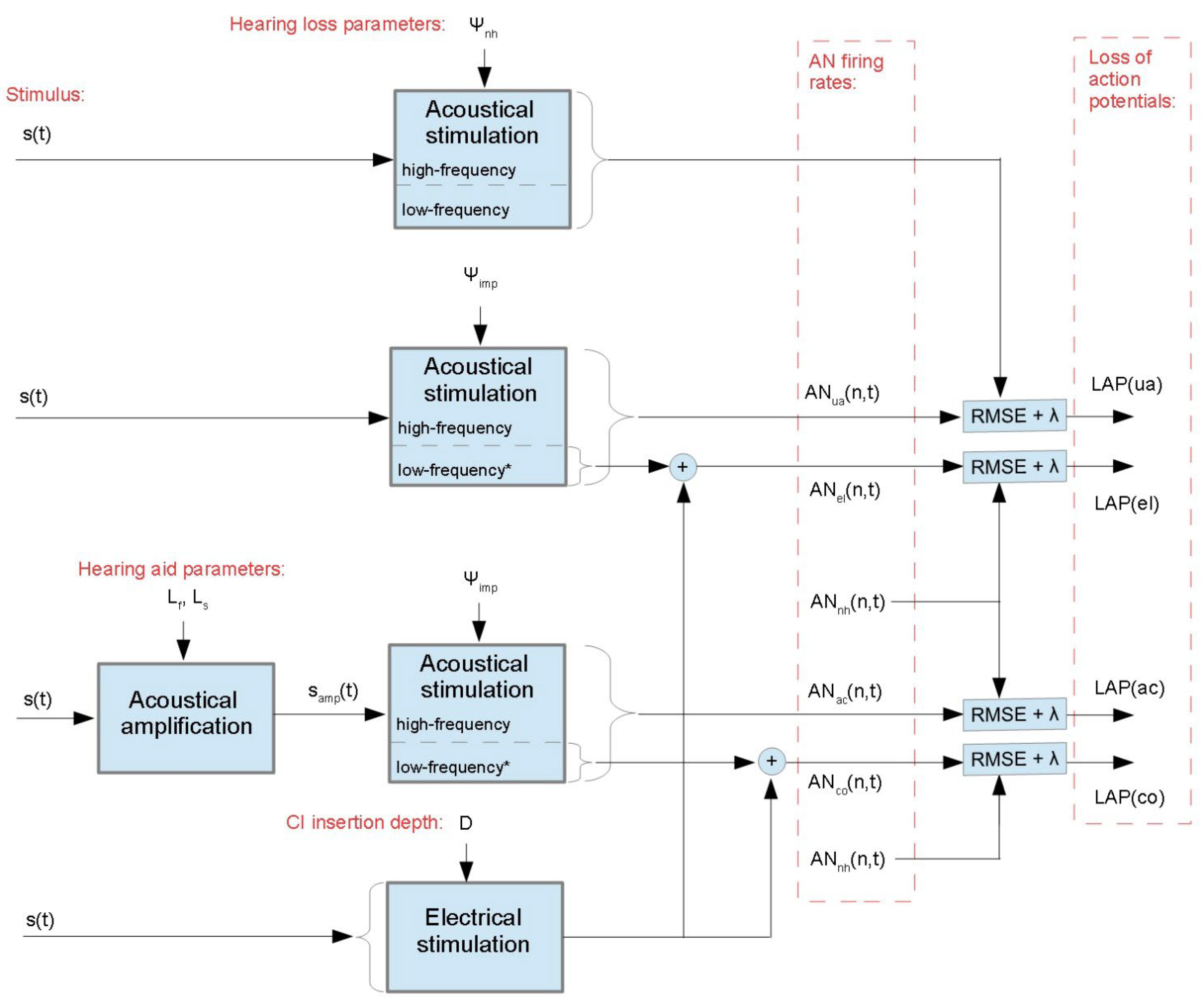
Figure 1 shows a block diagram overview of the modelling approach to predict AN firing rates for different hearing prosthesis options in a personalized way, as well as to obtain for each prosthesis option the LAP scores. First, the model of Verhulst et al. of acoustical stimulation was used three times with different hearing loss parameters $\mathsf{\Psi }$ and input stimuli [8]. The AN firing rates of the NH reference ${\mathrm{AN}}_{\mathrm{nh}}\left(\mathrm{n},\mathrm{t}\right)$ were obtained with hearing parameters reflecting NH (${\mathsf{\Psi }}_{\mathrm{nh}}$). The nerve signals of impaired (unaided) hearing ${\mathrm{AN}}_{\mathrm{ua}}\left(\mathrm{n},\mathrm{t}\right)$ were obtained with hearing parameters reflecting impaired hearing (${\mathsf{\Psi }}_{\mathrm{imp}}$). The input signal $\mathrm{s}\left(\mathrm{t}\right)$ was pre-amplified, owing to the amplification parameters ${\mathrm{L}}_{\mathrm{f}}$ and ${\mathrm{L}}_{\mathrm{s}}$ to obtain the firing rates of hearing with acoustical amplification ${\mathrm{AN}}_{\mathrm{ac}}\left(\mathrm{n},\mathrm{t}\right)$. Second, the model of Fredelake and Hohmann was used to obtain firing rates triggered by electrical stimulation ${\mathrm{AN}}_{\mathrm{el}}\left(\mathrm{n},\mathrm{t}\right)$ [13]. The fitting parameter was the CI insertion depth $\mathrm{D}$. The output was added to the low-frequency outputs of the models of acoustical stimulation ${\mathrm{AN}}_{\mathrm{ua}}\left(\mathrm{n},\mathrm{t}\right)$ to obtain firing rates including residual low-frequency hearing [17]. The residual hearing was simulated with stimuli that were attenuated by 20 dB [18]. To obtain firing rates for electrical stimulation combined with acoustic amplification, i.e., ${\mathrm{AN}}_{\mathrm{co}}\left(\mathrm{n},\mathrm{t}\right)$, the electrical stimulation model’s output was added to the low-frequency part of ${\mathrm{AN}}_{\mathrm{ac}}\left(\mathrm{n},\mathrm{t}\right)$. All nerve signals were compared to the NH reference, and their LAP scores were obtained. Details regarding the models of the firing rates, the acoustic amplification, the used stimuli, and the automatic fitting of the auditory prostheses are disclosed hereafter.

2.1. Models of the Auditory Nerve Firing Rates

2.1.1. Acoustical Stimulation

A biophysical model was used to predict stimuli firing rates of the AN fibers [8] from acoustic input. Version 1.2 of the model was used is and summarized as follows [12]. First, the acoustic stimulus passes a middle ear filter [19]. Second, the signal is put into an electrical equivalent circuit transmission-line model of the basilar membrane. The transmission line model is a cascade of serial impedances and parallel admittances [20]. The admittances are characterized by frequency- and level-dependent poles. Level dependence reflects the cochlear gain. At low stimulus levels, the poles are close to the imaginary axis of the s-plane, resulting in small-bandwidth high-gain cochlear filters. At high levels, the poles are apart from the imaginary axis, resulting in large-bandwidth low-gain cochlear filters. At levels in between, the pole positions are interpolated hyperbolically in a dynamics-compressing way. Tonotopy refers to a frequency–place mapping, i.e., low and high frequencies excite basilar membrane regions close to its apical and basal end, respectively. Subsequent processing is organized tonotopically. Third, the IHC membrane’s electrical potential is obtained from the deflections of the stereocilia, using a non-linear non-instantaneous electrical equivalent circuit with parallel branches for the direct mechanoelectrical transduction channel, as well as for the fast and the slow activating potassium channels of the cell [21]. Fourth, the synapse’s emission rate of neurotransmitters, i.e., the exocytosis rate, is another non-linear non-instantaneous function of the cell’s membrane electrical potential. Synapses with low, middle, and high exocytosis rates are modelled. In the absence of CS, each IHC is connected via synapses to ${\mathrm{N}}_{\mathrm{HSR}}=13$ high-rate fibers, ${\mathrm{N}}_{\mathrm{MSR}}=3$ middle-rate fibers, and ${\mathrm{N}}_{\mathrm{LSR}}=3$ low-rate fibers [22]. The fiber spontaneous rates before refractoriness are 1, 10, and 70 spikes/s, and their maximal rates are 800, 1000, and 3000 spikes/s, respectively. These rates are pre-refractoriness rates since they are well above the maximal steady-state rates. The adaptation of the exocytosis rate is modelled by a classic three-store diffusion model [23], and refractoriness is modelled by reducing the firing rate by short-term and long-term integrals over past firing rates [24].

2.1.2. Electrical Stimulation

A CI generates electrical impulses and injects them via its electrode array into the cochlea in order to trigger action potentials of the AN fibers. We used the continuous interleaved sampling (CIS) strategy to generate electrical impulses [25] and predicted the AN firing rates using the model of Fredelake and Hohmann [13].

First, the CIS strategy is explained. The signal is pre-processed with a head-related transfer function for frontal incidence of sound and are high-pass-filtered for pre-emphasis; then, automatic gain control is applied. The signal passes a 22-channel filter bank. The band envelopes are extracted by rectification and low-pass filtering and are input into a multi-band compressor that reduces the dynamic ranges. In each stimulation cycle, the eight channels with the largest activity are selected, which is referred to as 8-of-22 channel stimulation. The band envelopes of the selected channels modulate biphasic pulse trains, the pulses of which are interlaced in time for each channel to avoid simultaneous stimulation of multiple channels. The modulated biphasic pulse trains drive the electrode array.

Second, the firing rates of the ANs were predicted from the electrical pulse output by the electrode array using the model of Fredelake and Hohmann. The model is overviewed as follows. A spatial spread function predicts from the electrical pulses the effective input currents of the AN cells. The spatial spread function models the distribution of the electric field across the cochlea as a two-sided symmetrically decreasing exponential. In particular, the strength of the electric field decreases exponentially with distance from an electrode. The electrical fields of the individual electrodes are superimposed for all positions across the cochlea. The model of an AN cell comprises the models of the cell membrane, the membrane noise, the refractoriness of the cell, and latency and jitter of the action potentials. The cell membrane is modelled as an RC low-pass, taking a current as input and outputting the membrane depolarization potential. An action potential is triggered whenever the potential exceeds a threshold. To model the membrane noise, low-pass-filtered zero-mean Gaussian noise is added to the depolarization potential before thresholding. To model refractoriness after the release of an action potential, a cell has a dead time, after which the threshold potential is restored following an exponential function of time. Finally, the action potential is slightly delayed and jittered.

2.2. Acoustical Amplification

The open Master Hearing Aid (openMHA) toolbox was used to simulate multi-band compression of the acoustic signal [15,16]. Nine logarithmically spaced channel center frequencies ranging from 177 to 13,790 Hz were used. In each channel, low-level input signals up to 30 dB SPL were amplified using a low-level gain that is allowed to range from 0 to 60 dB. The gain decreased linearly up to input levels of 90 dB SPL, for which the gain was 0 dB. The low-level gain was controlled in a frequency-dependent way. In particular, frequency-flat and -sloping gain components $L_f$ and $L_s$ were used. For the four lowest frequency bands, i.e., 177, 305, 526, and 906 Hz, the low-level gains were equal to $L_f$, and for the five remaining bands, the low-level gains increased linearly with frequency. $L_s$ denotes the gain at the eighth frequency band, which was centered at 8 kHz.

2.3. Corpus Description

2.3.1. Stimuli

A microphone recording of a speaker uttering the word ‘nest’ was used as input. The word ‘nest’ was chosen because it contains a variety of phoneme types, while it is short enough for fast computation. The phoneme types were the nasal /n/, the vowel /e/, the fricative /s/, and the plosive /t/. The length of the recording was 320 ms. The average fundamental frequency was 114 Hz, and the frequencies of the first and second formants of the vowel were approximately 300 and 1450 Hz, respectively. A headworn microphone AKG HC 577 L and a portable recorder TASCAM DR-100 were used. The sampling frequency was 44.1 kHz, and the quantization resolution was 24 bits. To reflect input-level-dependent effects, the microphone recording was input to the model twice, i.e., with equivalent sound pressure levels set to 45 and 65 dB (20 µPa).

2.3.2. Characterization of Hearing Loss

A total of 1024 different hearing loss profiles was created. Each of the profiles reflected an individual subject. Groups of subjects were distinguished by the presence or absence of CGL, IHCL, and CS, which resulted in eight groups of 128 subjects each. For subjects with CGL and/or IHCL, the flat components were drawn from uniform distributions ranging from 0 to 35 and 0 to 60 dB, respectively. The slopes were also drawn from uniform distributions, which were truncated subject-wise to keep ${\mathrm{O}}_{\mathrm{f}}\ge {\mathrm{O}}_{\mathrm{s}}$ and ${\mathrm{I}}_{\mathrm{f}}\ge {\mathrm{I}}_{\mathrm{s}}$. For subjects with CS, the average number of active fibers per IHC ${\mathrm{N}}_{\mathrm{fib}}$ was drawn from a beta distribution ranging from 0 to 19.

Table 1. Distributions of hearing loss parameters $\mathsf{\Psi }=\left\{{\mathrm{I}}_{\mathrm{f}},{\mathrm{I}}_{\mathrm{s}},{\mathrm{O}}_{\mathrm{f}},{\mathrm{O}}_{\mathrm{s}},{\mathrm{N}}_{\mathrm{fib}}\right\}$ with regard to subject groups.

		Hearing Loss Parameters
		Cochlear Gain Loss		Loss of Inner Hair Cells		Cochlear Synaptopathy
		Flat Component	Sloping Component	Flat Component	Sloping Component	Number of Active Fibers
		${\mathrm{O}}_{\mathrm{f}}$ (dB)	${\mathrm{O}}_{\mathrm{s}}$ (dB)	${\mathrm{I}}_{\mathrm{f}}$ (dB)	${\mathrm{I}}_{\mathrm{s}}$ (dB)	${\mathrm{N}}_{\mathrm{fib}}$
Subject groups	NH	0	0	0	0	19
	CS	0	0	0	0	$19\cdot \mathrm{Beta}\left(1, 0.5\right)$
	IHCL	0	0	$\mathcal{U}\left(0, 60\right)$	$\mathcal{U}\left({\mathrm{I}}_{\mathrm{f}}, 60\right)$	19
	IHCL + CS	0	0	$\mathcal{U}\left(0, 60\right)$	$\mathcal{U}\left({\mathrm{I}}_{\mathrm{f}}, 60\right)$	$19\cdot \mathrm{Beta}\left(1, 0.5\right)$
	CGL	$\mathcal{U}\left(0, 35\right)$	$\mathcal{U}\left({\mathrm{O}}_{\mathrm{f}}, 35\right)$	0	0	19
	CGL + CS	$\mathcal{U}\left(0, 35\right)$	$\mathcal{U}\left({\mathrm{O}}_{\mathrm{f}}, 35\right)$	0	0	$19\cdot \mathrm{Beta}\left(1, 0.5\right)$
	CGL + IHCL	$\mathcal{U}\left(0, 35\right)$	$\mathcal{U}\left({\mathrm{O}}_{\mathrm{f}}, 35\right)$	$\mathcal{U}\left(0, 60\right)$	$\mathcal{U}\left({\mathrm{I}}_{\mathrm{f}}, 60\right)$	19
	CGL + IHCL + CS	$\mathcal{U}\left(0, 35\right)$	$\mathcal{U}\left({\mathrm{O}}_{\mathrm{f}}, 35\right)$	$\mathcal{U}\left(0, 60\right)$	$\mathcal{U}\left({\mathrm{I}}_{\mathrm{f}}, 60\right)$	$19\cdot \mathrm{Beta}\left(1, 0.5\right)$

For cochlear gain loss (CGL) and loss of IHCs (IHCL), frequency-flat and -sloping components were either 0 dB or drawn from uniform distributions. For cochlear synaptopathy (CS), the number of active fibers per IHC was either 19 or drawn from a beta distribution. The eight subject groups reflect all possible combinations of the presence or absence of CGL, IHCL, and CS.

summarizes distributions of hearing loss parameters $\mathsf{\Psi }$ with regard to subject groups.

CGL was simulated by moving the poles of the basilar membrane transition line model described in Section 2.1.1. In particular, the positions of low-level poles of the basilar membrane transmission line model are modified to reflect individual frequency-specific CGLs, i.e., a frequency profile in the dB hearing level (HL) [8]. The low-level poles are moved toward the high-level poles in the case of CGL.

To simulate IHCL, i.e., damage of the IHCs, firing rates of single nerve fibers were set to zero in order to match a target density of residual functional IHCs. In particular, IHCL was simulated by switching off the outputs of randomly selected individual IHCs. The switched-off IHCs were selected using a Bernoulli distribution. The distribution’s parameter $\mathrm{p}$ was the probability of switching off a particular IHC. The probability was allowed to vary with frequency, owing to the flat and sloping component of IHCL, i.e., ${\mathrm{I}}_{\mathrm{f}}$ and ${\mathrm{I}}_{\mathrm{s}}$. The probability of the flat component $\mathrm{p}=1-{10}^{\left(-{\mathrm{I}}_{\mathrm{f}}/20\right)}$. The probability increased linearly for frequencies exceeding 1 kHz and went through ${\mathrm{p}}_8=1-{10}^{\left(-{\mathrm{I}}_{\mathrm{s}}/20\right)}$ at 8 kHz. It should be noted that the components regarding IHCL did not correspond to dB HL, but instead rather referred to spatial density of damaged IHCs.

To simulate CS, i.e., damage of the synapses between the IHCs and the AN, the numbers of synapses were reduced for the IHCs that were not switched off due to IHCL. For modelling CS, if $19>{\mathrm{N}}_{\mathrm{fib}}\ge 16$, only the number of LSR synapses was reduced, i.e., ${\mathrm{N}}_{\mathrm{fib}}^{\mathrm{LSR}}=19-{\mathrm{N}}_{\mathrm{fib}}$, ${\mathrm{N}}_{\mathrm{fib}}^{\mathrm{MSR}}=3$, and ${\mathrm{N}}_{\mathrm{fib}}^{\mathrm{HSR}}=13$. If $16>{\mathrm{N}}_{\mathrm{fib}}\ge 13$, no LSR synapses were left, and the number of MSR synapses was reduced, i.e., ${\mathrm{N}}_{\mathrm{fib}}^{\mathrm{LSR}}=0$, ${\mathrm{N}}_{\mathrm{fib}}^{\mathrm{MSR}}=16-{\mathrm{N}}_{\mathrm{fib}}$, and ${\mathrm{N}}_{\mathrm{fib}}^{\mathrm{HSR}}=13$. If $13>{\mathrm{N}}_{\mathrm{fib}}$, no LSR and MSR synapses were left, and the number of HSR synapses was reduced, i.e., ${\mathrm{N}}_{\mathrm{fib}}^{\mathrm{LSR}}={\mathrm{N}}_{\mathrm{fib}}^{\mathrm{MSR}}=0$ and ${\mathrm{N}}_{\mathrm{fib}}^{\mathrm{HSR}}={\mathrm{N}}_{\mathrm{fib}}$.

2.4. Fitting of the Hearing Prostheses

The CI and the hearing aid parameters were fit to individual hearing loss profiles by minimizing the normalized root mean square difference reflecting the ‘loss of action potentials’, i.e.,

$$\mathrm{LAP}\left(\mathsf{\Omega }\right)=\frac{\sqrt{\overline{{\left({\mathrm{AN}}_{\mathrm{nh}}-{\mathrm{AN}}_{\mathsf{\Omega }}\right)}^2}}}{\sqrt{\overline{{\mathrm{AN}}_{\mathrm{nh}}^2}}}+{\mathsf{\lambda }}_{\mathsf{\Omega }},$$

(1)

where ${\mathrm{AN}}_{\mathsf{\Omega }}\left(\mathrm{n},\mathrm{t}\right)$ are AN firing rates predicted for prosthesis option $\mathsf{\Omega }\in \left\{\mathrm{ua},\mathrm{ac},\mathrm{el},\mathrm{co}\right\}$, i.e., unaided hearing, acoustic amplification, electrical stimulation, and electrical stimulation combined with acoustic amplification. ${\mathsf{\lambda }}_{\mathsf{\Omega }}$ is a parameter to adjust LAP for the ‘costs’ of acoustical amplification and cochlear implantation. The cost parameter for unaided hearing ${\mathsf{\lambda }}_{\mathsf{\Omega }=\mathrm{ua}}=0$, for sole acoustical amplification $0\le {\mathsf{\lambda }}_{\mathsf{\Omega }=\mathrm{ac}}\le 0.1$, for sole electrical stimulation $0\le {\mathsf{\lambda }}_{\mathsf{\Omega }=\mathrm{el}}\le 0.25$, and for electrical stimulation combined with acoustical amplification ${\mathsf{\lambda }}_{\mathsf{\Omega }=\mathrm{co}}={\mathsf{\lambda }}_{\mathsf{\Omega }=\mathrm{ac}}+{\mathsf{\lambda }}_{\mathsf{\Omega }=\mathrm{el}}$. The default values were ${\mathsf{\lambda }}_{\mathsf{\Omega }=\mathrm{ac}}=0.01$, and ${\mathsf{\lambda }}_{\mathsf{\Omega }=\mathrm{el}}=0.05$. The LAP was typically between 0 (NH) and 1 (deafness). LAP was obtained for stimulus levels of 45 and 65 dB (20 µPa) individually, and the mean was taken. Before the computation of $\mathrm{LAP}$, the spontaneous rates were subtracted from all AN firing rates. The place resolution was 120 nerve fibers, and the time resolution was 1.4 ms.

The fitting parameters for the acoustic amplification were the frequency-flat and the frequency-sloping components of the low-level gain, i.e., ${\mathrm{L}}_{\mathrm{f}}$ and ${\mathrm{L}}_{\mathrm{s}}$. The optimal parameters were obtained as $\left[{\mathrm{L}}_{\mathrm{f}}^{\mathrm{opt}},{\mathrm{L}}_{\mathrm{s}}^{\mathrm{opt}}\right]= \mathrm{argmin}\left[\mathrm{LAP}\left({\mathrm{L}}_{\mathrm{f}},{\mathrm{L}}_{\mathrm{s}}\right)\right]$, where $\mathrm{LAP}$ was obtained with ${\mathrm{AN}}_{\mathsf{\Omega }=\mathrm{ac}}$. ${\mathrm{L}}_{\mathrm{f}}$ and ${\mathrm{L}}_{\mathrm{s}}$ were jointly optimized in two loops. In each loop, first ${\mathrm{L}}_{\mathrm{f}}$ was optimized using golden-section search with parabolic interpolation, and then ${\mathrm{L}}_{\mathrm{s}}$. In the first loop, the minimization was coarse, i.e., with stopping criterion tolerances of 5 dB for both ${\mathrm{L}}_{\mathrm{f}}$ and ${\mathrm{L}}_{\mathrm{s}}$, and 1% for $\mathrm{LAP}$. In the second loop, ${\mathrm{L}}_{\mathrm{f}}$ and ${\mathrm{L}}_{\mathrm{s}}$ were fine-tuned, i.e., with stopping criterion tolerances of 0.5 dB and 0.1%, respectively. ${\mathrm{L}}_{\mathrm{f}}$ and ${\mathrm{L}}_{\mathrm{s}}$ were constraint to 0 and 60 dB, and ${\mathrm{L}}_{\mathrm{f}}\le { \mathrm{L}}_{\mathrm{s}}$.

The fitting parameter of the electrical stimulation was the electrode array’s insertion depth $\mathrm{D}$. The optimal insertion depth was obtained as ${\mathrm{D}}^{\mathrm{opt}}= \mathrm{argmin}\left[{\mathrm{r}}_{\mathrm{d}}\left(\mathrm{D}\right)\right]$. $\mathrm{D}$ was optimized using golden-section search with parabolic interpolation, using a stopping criterion tolerance of 0.5 mm. $\mathrm{D}$ was constraint to 19 and 29 mm, which corresponded to apex-to-tip distances ranging from 16 to 6 mm in a 35 mm cochlea.

2.5. Statistics and Classification

First, descriptive statistics regarding the best prosthesis option (minimum LAP) with respect to hearing loss types were obtained. All combinations of IHCL, GCL, and CS were considered.

Second, classifiers were trained to predict a binary group allocation, i.e., ‘implant’ versus ‘no implant’. Subjects for which the minimum LAP was observed with either unaided hearing or sole acoustic amplification were allocated to the group ‘no implant’. The remaining subjects were allocated to the group ‘implant’. For these subjects, the minimum LAP was observed with either sole electrical stimulation or electrical stimulation combined with acoustic amplification.

Third, single- and multi-predictor classification was used. Regarding single-predictor classification, cut-off thresholds were estimated using ROC curves. Regarding multi-predictor classification, logistic regression and a support vector machine with a quadratic kernel were trained independently of each other. The logistic regression model and the support vector machine were trained using as predictors the hearing loss parameters ${\mathrm{I}}_{\mathrm{f}}$ (dB), ${\mathrm{I}}_{\mathrm{s}}$ (dB), ${\mathrm{O}}_{\mathrm{f}}$ (dB), ${\mathrm{O}}_{\mathrm{s}}$ (dB), and ${\mathrm{N}}_{\mathrm{fib}}$. Tenfold cross-validation was applied.

3. Results

This section is structured as follows. In Section 3.1, descriptive statistics regarding the number of subjects with respect to their types of hearing loss and their predicted best hearing prosthesis are presented. In Section 3.2, four case studies are presented, i.e., detailed comparisons of AN signals of four subjects, and bar charts reflecting personalized hearing prosthesis recommendations. Implantation recommendations using single- and multi-predictor classification are presented in Section 3.3 and Section 3.4, respectively.

3.1. Best Hearing Prostheses versus Hearing Loss Types

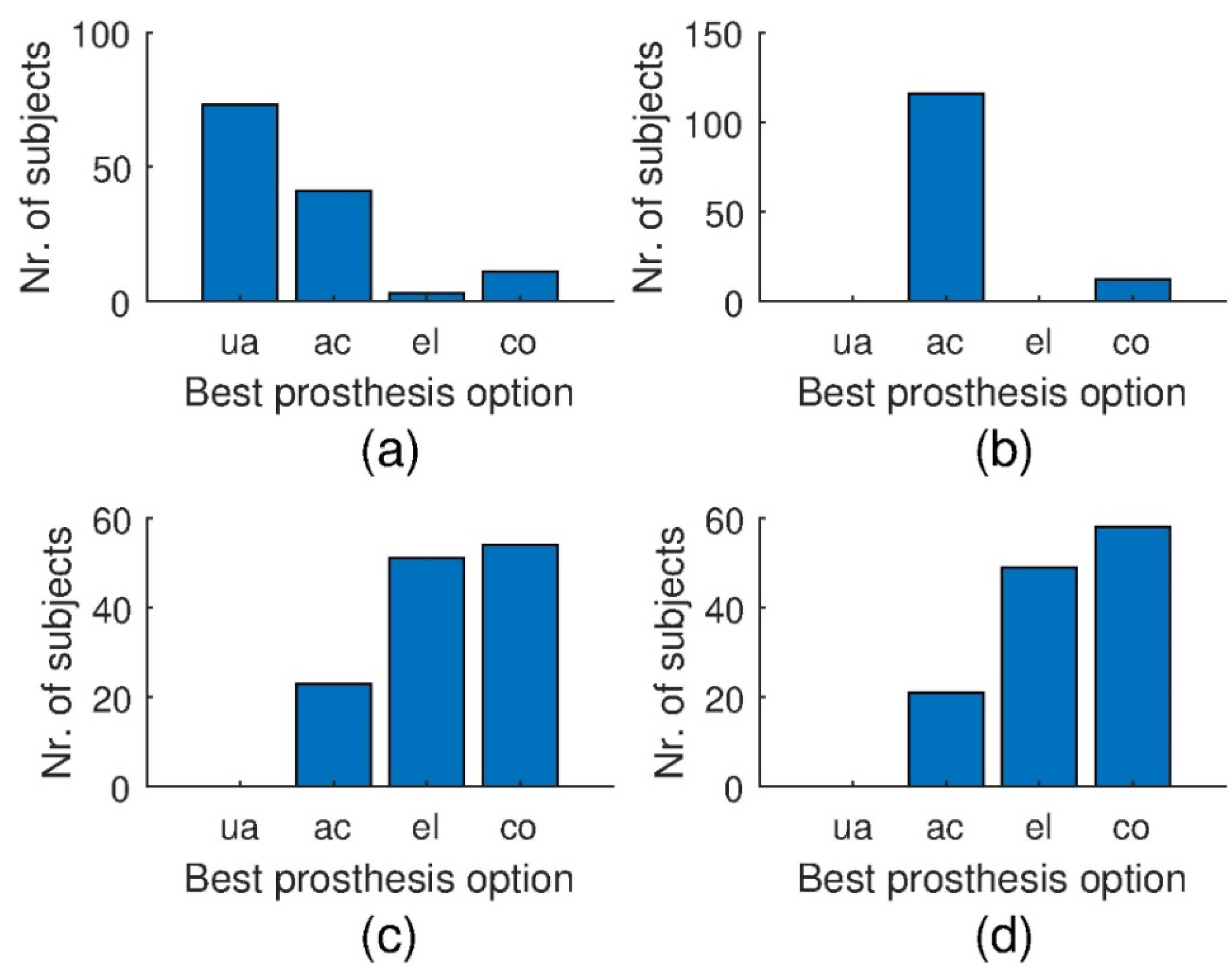
Figure 2 and Figure 3 show bar charts reporting numbers of subjects with regard to their individually predicted best hearing prosthesis option, as well as the type of hearing loss. For each subject, the best prosthesis option is the one with the minimum LAP. Figure 2 and Figure 3 report numbers of subjects without and with CS, respectively. For NH and sole CGL (first row of Figure 2), all subjects were predicted to have minimum LAP for unaided hearing and sole acoustical amplification, respectively. This provides a sanity check for NH subjects, as well as suggests that sole CGL is most appropriately compensated using sole acoustical amplification. For most subjects with IHCL (with or without additional CGL), electrical stimulation with and without additional acoustical amplification appear to be the best options for approximately equally many subjects, followed by sole acoustical amplification. None of the subjects with IHCL were suggested to remain unaided.

For sole CS (Figure 3, top left), most subjects are suggested to stay without a prosthesis, followed by sole acoustical amplification. Some subjects, presumably the ones with the most severe CS, are suggested to be implanted. For CS with CGL (top right), the majority of subjects are suggested to get a hearing aid, while some subjects, presumably the ones with severe CS, are suggested to receive a combined prosthesis. For subjects with IHCL and CS (bottom row), the results are comparable to the results for subjects with IHCL and no CS (bottom row of Figure 2).

3.2. Case Studies

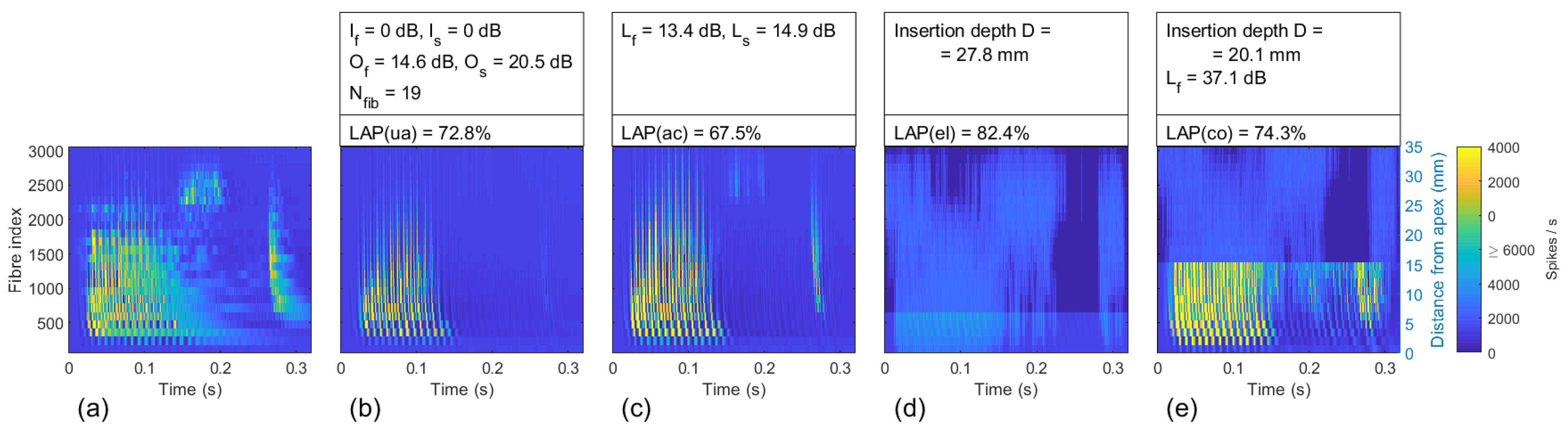
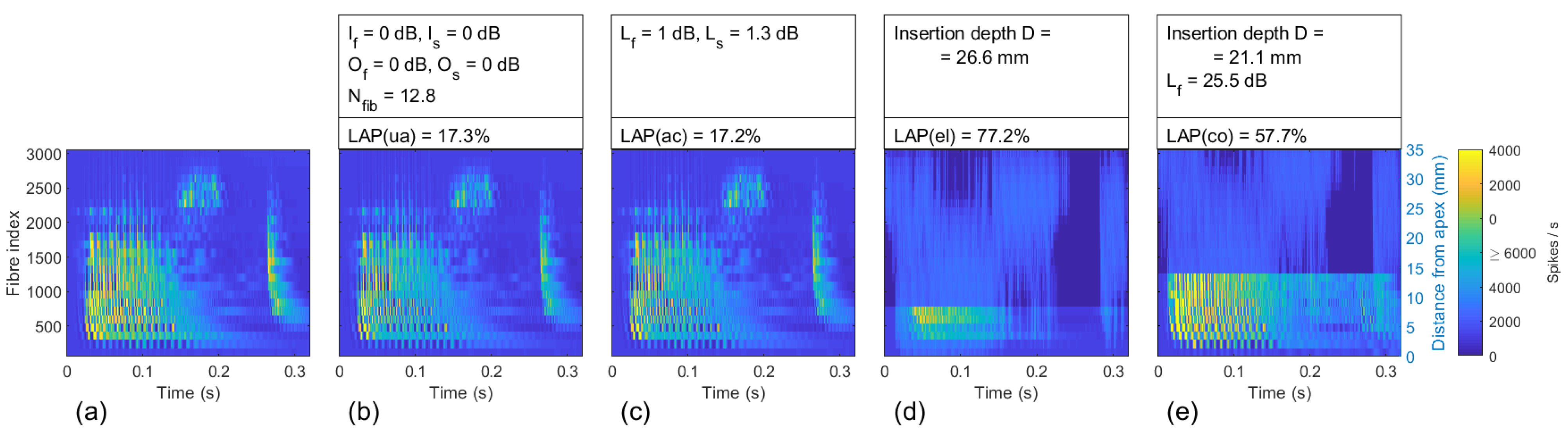
In the following, a few case studies regarding different types of hearing loss are presented. Firing rates are depicted with respect to fiber index (y-axes) and time (x-axes). The fibers are ordered by their origin from apex (bottom) to base (top), which corresponds to low and high frequencies, respectively. Figure 4, Figure 5, Figure 6 and Figure 7 show firing rates for (a) NH, i.e., the reference; (b) unaided hearing, i.e., the baseline; (c) hearing with sole acoustical amplification; (d) hearing with sole electrical stimulation, including residual hearing at low frequencies; and (e) electrical stimulation combined with acoustical amplification. In addition, hearing loss parameters, personalized fitting parameters, and LAPs are shown on the top of the images. In NH, three major clusters of AN firings are observed. First, the largest cluster at the bottom left of the image corresponds to the first two phonemes /n/ and /e/ of the stimulus. The second cluster is located at the top in the middle, i.e., around fiber index 2500 and 0.2 s. It corresponds to the third phoneme, /s/. Finally, the third cluster is shown on the right. It is located at around 0.28 s, and ranges from approximately fiber 500 to fiber 2500. Moreover, a few speckles are observed between the clusters.

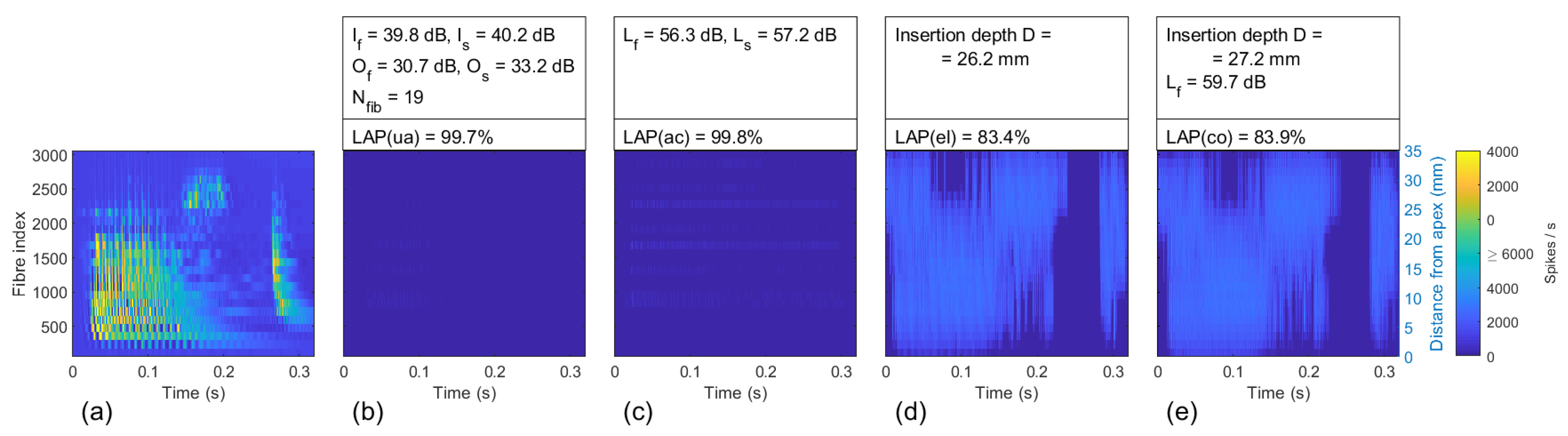
Figure 4 shows the results for a subject with severe to profound hearing impairment. In particular, most of the IHCs were damaged, which is reflected by ${\mathrm{I}}_{\mathrm{f}}$ = 39.8 dB and ${\mathrm{I}}_{\mathrm{s}}$ = 40.2 dB. Moreover, severe CGL was present, which is reflected by ${\mathrm{O}}_{\mathrm{f}}$ = 30.7 dB and ${\mathrm{O}}_{\mathrm{s}}$ = 33.2 dB. The unaided LAP(ua) = 99.7% reflected hearing loss close to deafness. With sole acoustical amplification, no improvement was achieved, i.e., LAP(ac) = 99.8%, even with large gain factors $L_f$ = 56.3 dB and $L_s$ = 57.2 dB. Smaller LAPs were obtained for the remaining two options, i.e., LAP(el) = 83.4% and LAP(co) = 83.9%. The combination with acoustical amplification did not outperform sole electrical stimulation, which was due to the absence of substantial residual hearing at low frequencies.

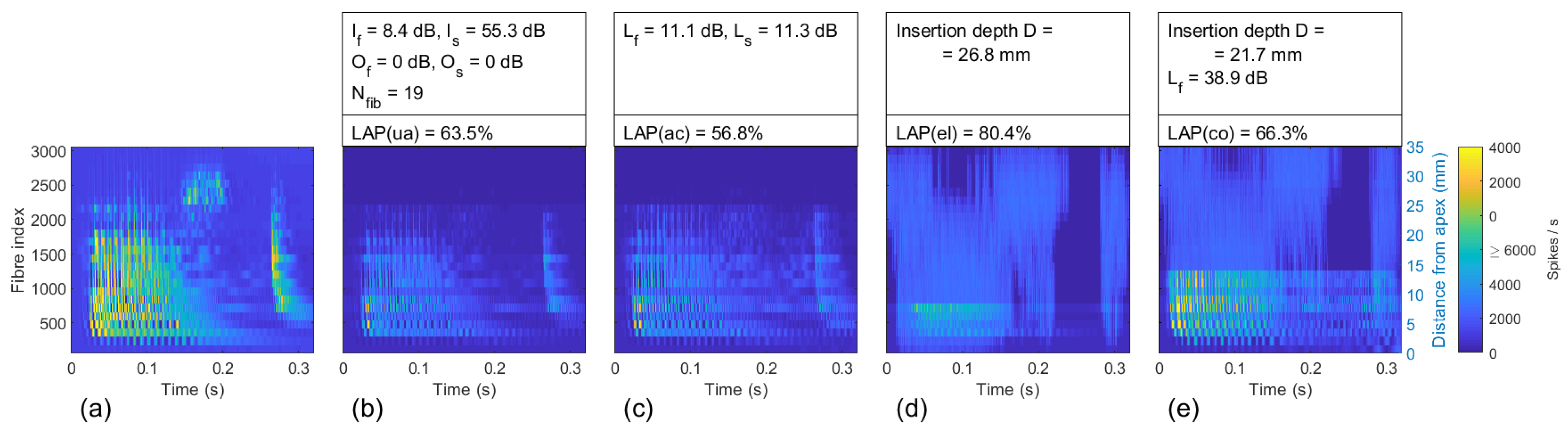
Figure 5 reports results for a subject with a complete loss of IHCs in a basal dead region, and a partly loss of IHCs in the remaining cochlear regions. The former is reflected by ${\mathrm{I}}_{\mathrm{s}}$ = 55.3 dB, and the latter by ${\mathrm{I}}_{\mathrm{f}}$ = 8.4 dB. The hearing loss is reflected in (b) by the absence of firing of high frequency fibers, i.e., missing of the /s/-cluster, as well as substantial decrease in neural activity in the lower frequency region. The unaided loss of action potentials LAP(ua) = 63.5%. A better option is acoustic amplification (LAP(ac) = 56.8%). The LAP is larger for options involving cochlear implantation, i.e., 80.4% and 66.3%.

Figure 6 reports results for a subject with a moderate flat component, as well as a larger sloping component of CGL. The LAP(ua) was 72.8%, which reflects significant loss of hearing. The speckles that are visible in the NH reference appear to be suppressed in unaided hearing (b). Moreover, the /s/- and /t/-clusters of nerve firings associated with the fricative /s/ and the plosive /t/ appear to be particularly faint in (b). Loss of frequency selectivity associated with CGL is reflected by the pronounced vertical structures shown in (b), which was due to a broadening of cochlear tuning. Acoustic amplification shown in (c) appeared to enable partial recovery of the /s/- and /t/-clusters, but the cochlear tuning remained broadened. The LAP(ac) was 67.5%. The LAPs of the hearing prosthesis options involving implantation (d, e) were larger, i.e., 82.4% and 74.3%, respectively, which reflects the fact that high-frequency AN firing rates triggered by electrical stimulation are more artificial/blurred than firing rates of unaided hearing or with acoustic amplification in this subject.

Figure 7 shows results for a subject with moderate to severe CS. In particular, an average of 12.8 functional fibers with high spontaneous rates existed for each IHC, whereas synapses releasing into low and middle spontaneous rate fibers were damaged. In (b), the unaided scenario, the predicted LAP was 17.3%. Marginal improvement was predicted for sole acoustic amplification (LAP = 17.2%). For (e), i.e., electrical stimulation combined with acoustic amplification, the LAP was much larger, i.e., 57.7%, and for sole electrical stimulation (d), the LAP was even larger, i.e., 77.2%.

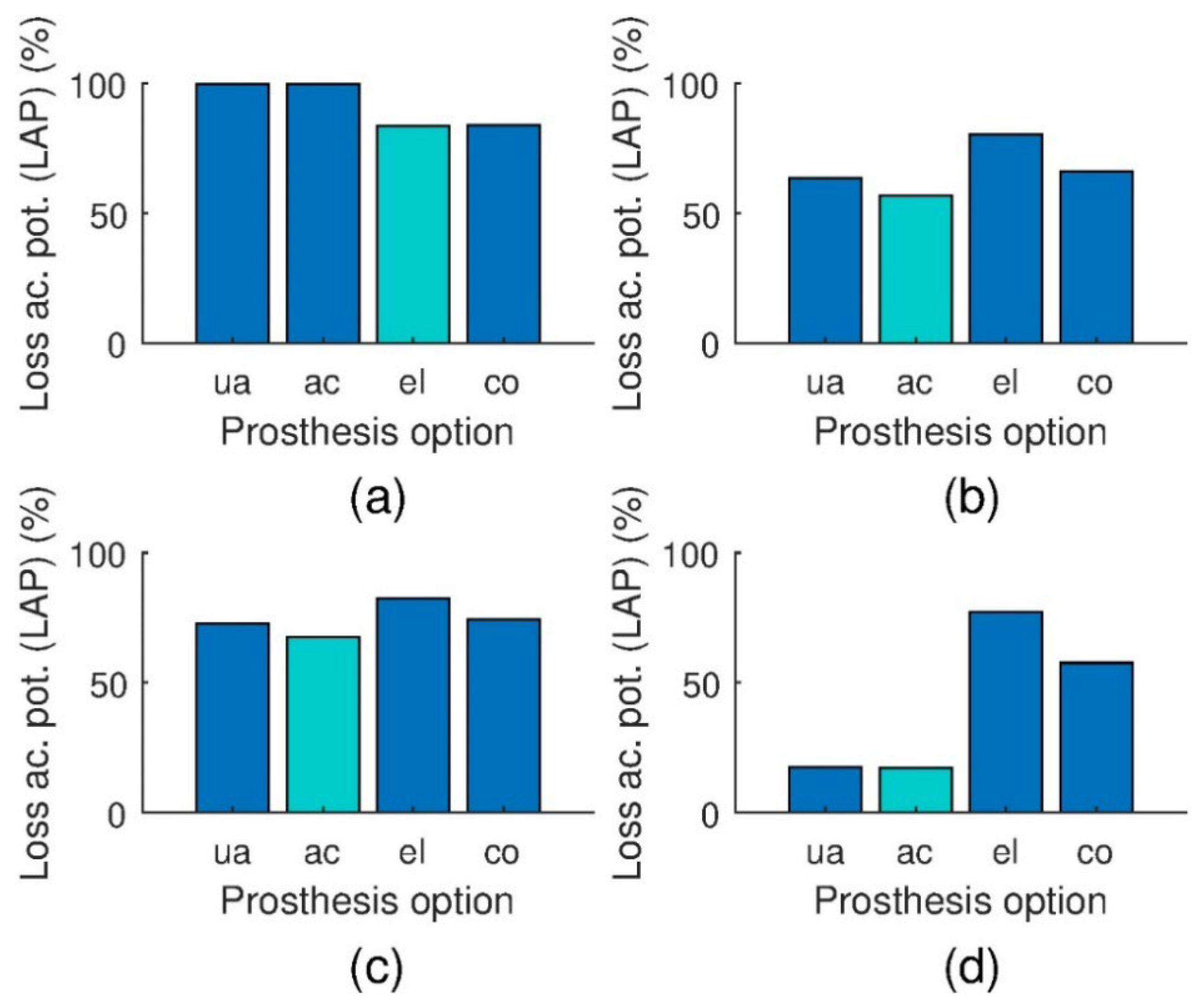
Figure 8 summarizes for each of the reported cases the LAPs in a bar chart. The bar charts may reflect recommendation weights of particular hearing prosthesis options. Shorter bars reflect stronger recommendations, and the color of the shortest bar was made distinct. Such bar charts are suggested to be displayed to clinicians by a possible prospective decision support system.

3.3. Implantation Recommendation Based on Single Hearing Loss Parameters

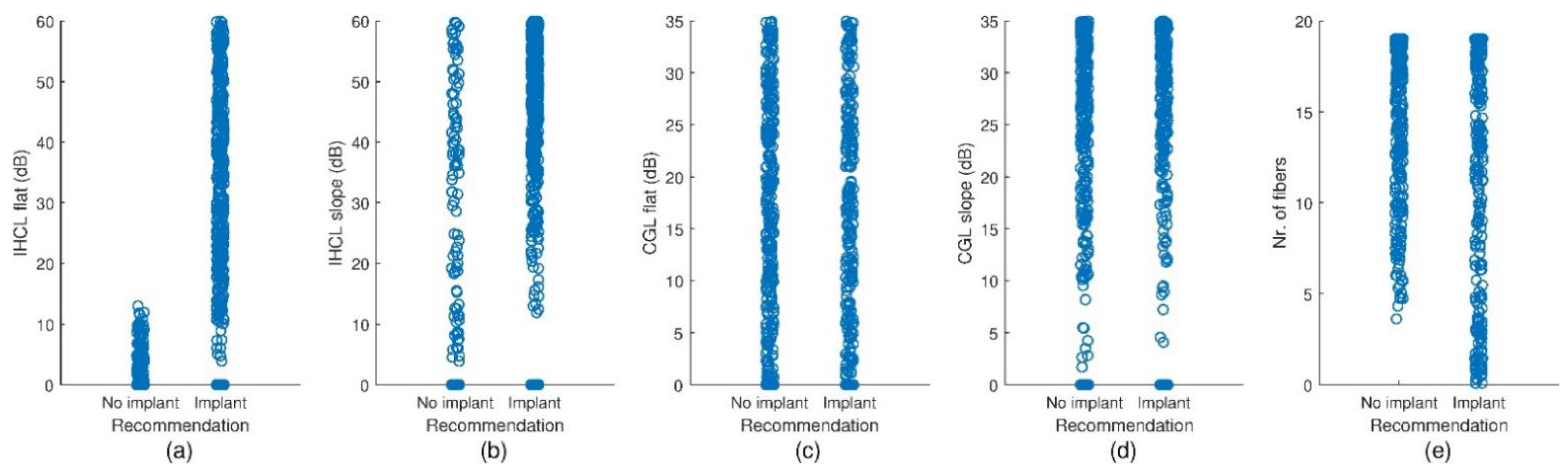
Figure 9 shows scatterplots of individual hearing loss parameters that are grouped with regard to the predicted recommendation ‘implant’/‘no implant’. Each circle corresponds to one subject. To improve visibility, a small jitter was added to the positions along the x-axes. The largest differences were observed in IHCL parameters. In particular, the ‘no implant’ subjects appeared to cluster below 10 dB, whereas the majority of the ‘implant’ subjects appeared to cluster above 10 dB. ‘No implant’ subjects with large ${\mathrm{I}}_{\mathrm{s}}$ values existed, but large ${\mathrm{I}}_{\mathrm{s}}$ values were much more frequent in the ‘implant’ subject group. Differences between the groups were also observed for ${\mathrm{N}}_{\mathrm{fib}}$. In particular, ‘no implant’ subjects with few functional synapses were rare. In contrast, group effects of CGL parameters appeared to be negligible. A more formal approach towards thresholding-based distinction of ‘implant’ and ‘no implant’ subjects using single hearing loss parameters is reported in the subsequent paragraph.

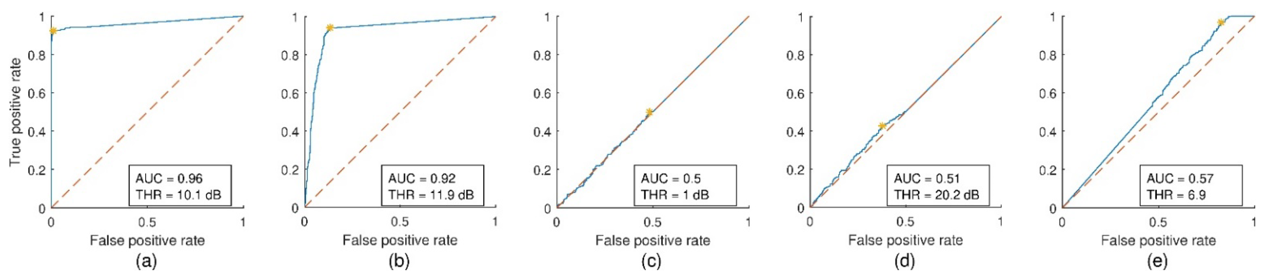
Figure 10 shows the ROC curves for the distributions shown in Figure 9. The area under the curves (AUC) were largest for the IHCL parameters ${\mathrm{I}}_{\mathrm{f}}$ and ${\mathrm{I}}_{\mathrm{s}}$, i.e., 0.96 and 0.92, respectively, reflecting large differences between these parameters in the ‘implant’ and ‘no implant’ group. The cut-off thresholds of ${\mathrm{I}}_{\mathrm{f}}$ and ${\mathrm{I}}_{\mathrm{s}}$ were estimated as 10.1 dB and 11.9 dB, respectively, corresponding to approximately 69% and 75% of damaged IHCs, respectively. The asterisks and thresholds THR refer to cut-off threshold classification. The optima of THR were found by maximizing the perpendicular distance between the line of equality (dashed line) and the curve. The AUC was substantially smaller for the CS parameter, i.e., 0.57, and even smaller for the CGL parameters, i.e., 0.5 and 0.51.

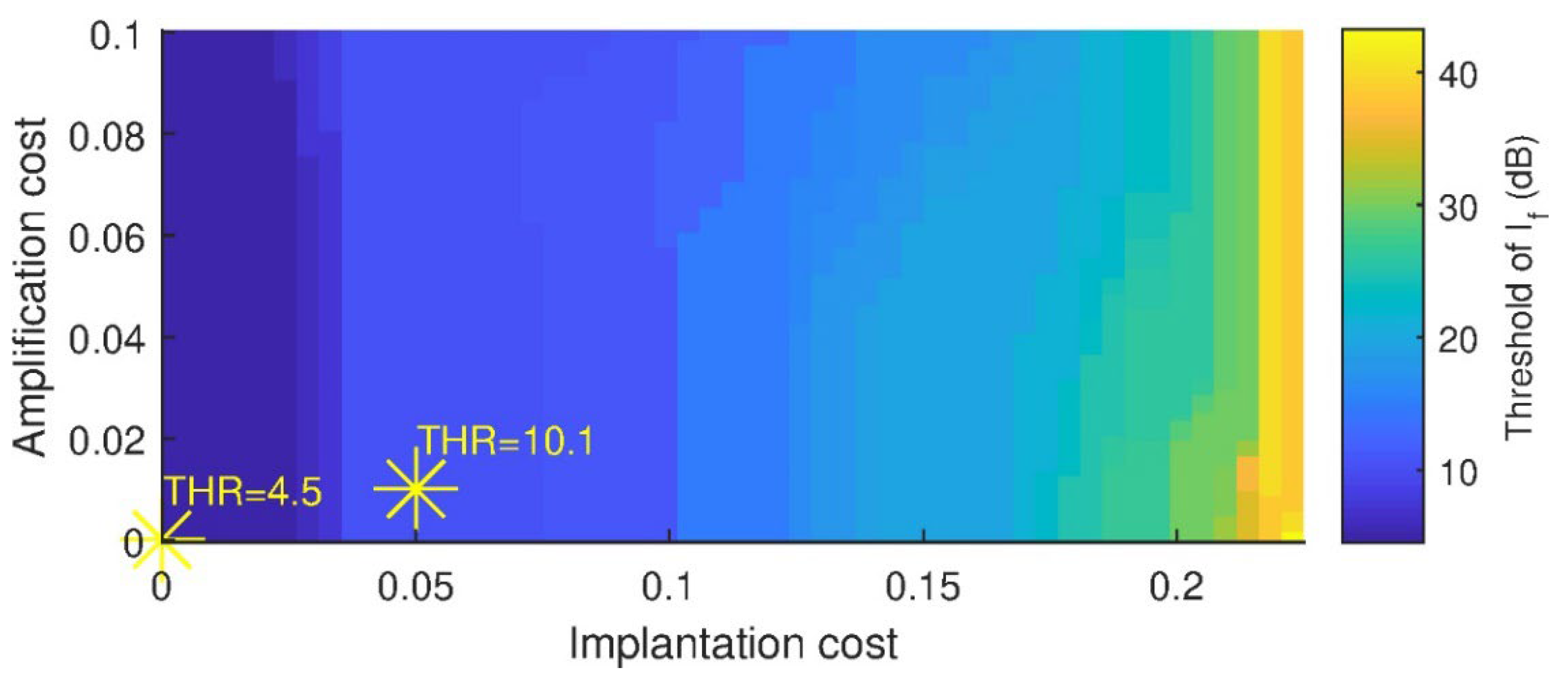
Figure 11 shows the optimal cut-off threshold of ${\mathrm{I}}_{\mathrm{f}}$ color-coded with respect to amplification cost ${\mathsf{\lambda }}_{\mathrm{amp}}$ and implantation cost ${\mathsf{\lambda }}_{\mathrm{imp}}$. The implantation cost influenced the threshold more strongly than the amplification cost. Two operating points are shown (yellow asterisks). One was at ${\mathsf{\lambda }}_{\mathrm{amp}}=0.01$ and ${\mathsf{\lambda }}_{\mathrm{amp}}=0.05$, where THR = 10.1 dB. The cost parameters of this operating point have been used throughout the manuscript. For comparison, the other operating point is shown at ${\mathsf{\lambda }}_{\mathrm{amp}}={\mathsf{\lambda }}_{\mathrm{imp}}=0$, where THR = 4.5 dB.

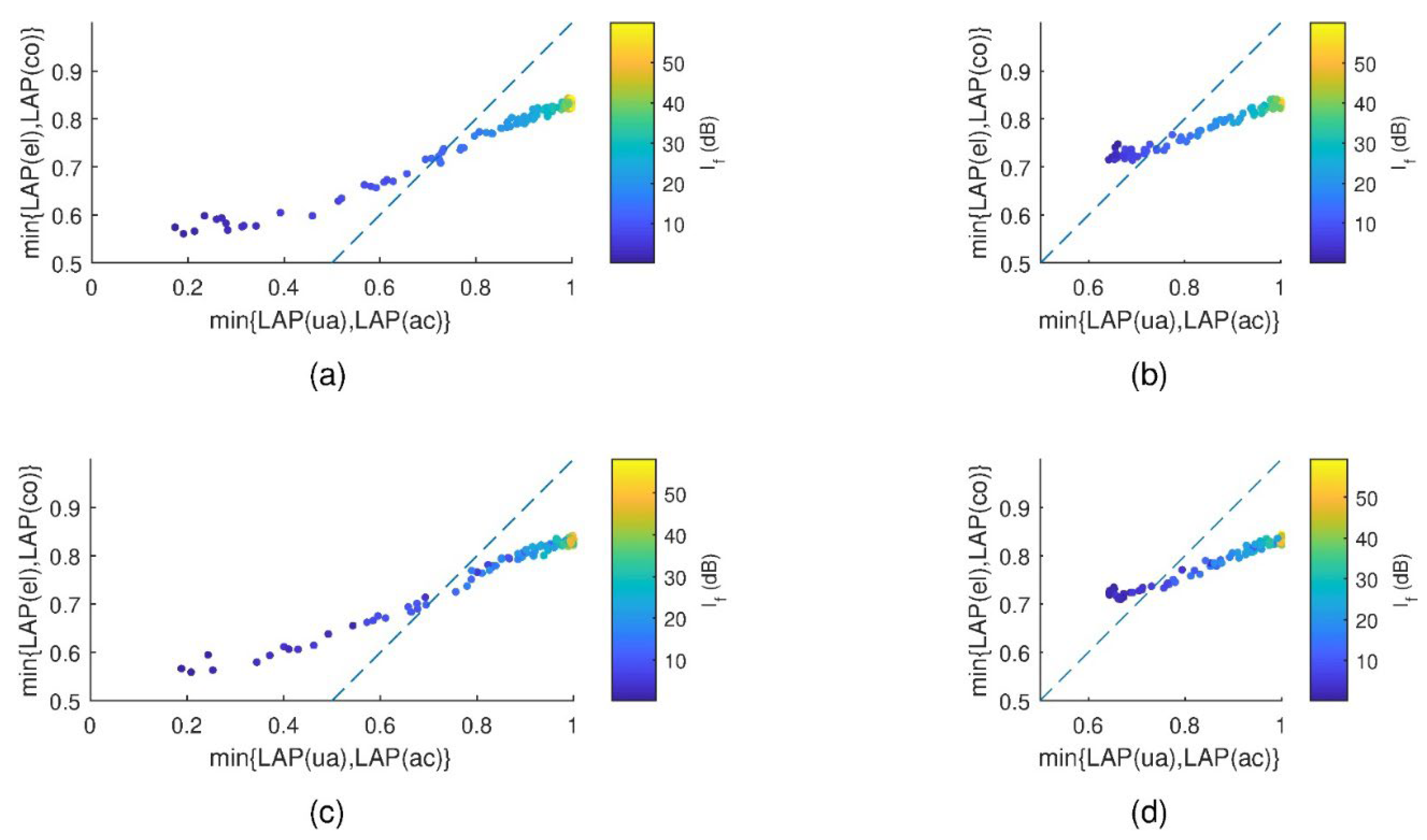
Figure 12 shows scatter plots of the minimum LAP score achieved with and without implantation. The dashed lines are the lines of equality, which were the boundary for the ‘implant’/‘no implant’ decision. The IHCL was color-coded. Each dot reflects one subject. Only subjects with IHCL are reported. The plots show distinct types of hearing loss, i.e., (a) IHCL, (b) CGL + IHCL, (c) IHCL + CS, and (d) CGL + IHCL + CS. A clear relationship between the ${\mathrm{I}}_{\mathrm{f}}$ and the position across the coordinate systems was observed. In particular, subjects with a small ${\mathrm{I}}_{\mathrm{f}}$ tended to lie to the left of the line of equality, and vice versa. Two distinct patterns were observed in the plots with and without CGL, i.e., for smallest ${\mathrm{I}}_{\mathrm{f}}$, subjects with CGL were closer to the line of equality than subjects without CGL, which reflects that the lowest possible LAP was larger for CGL subjects’ than for subjects without CGL.

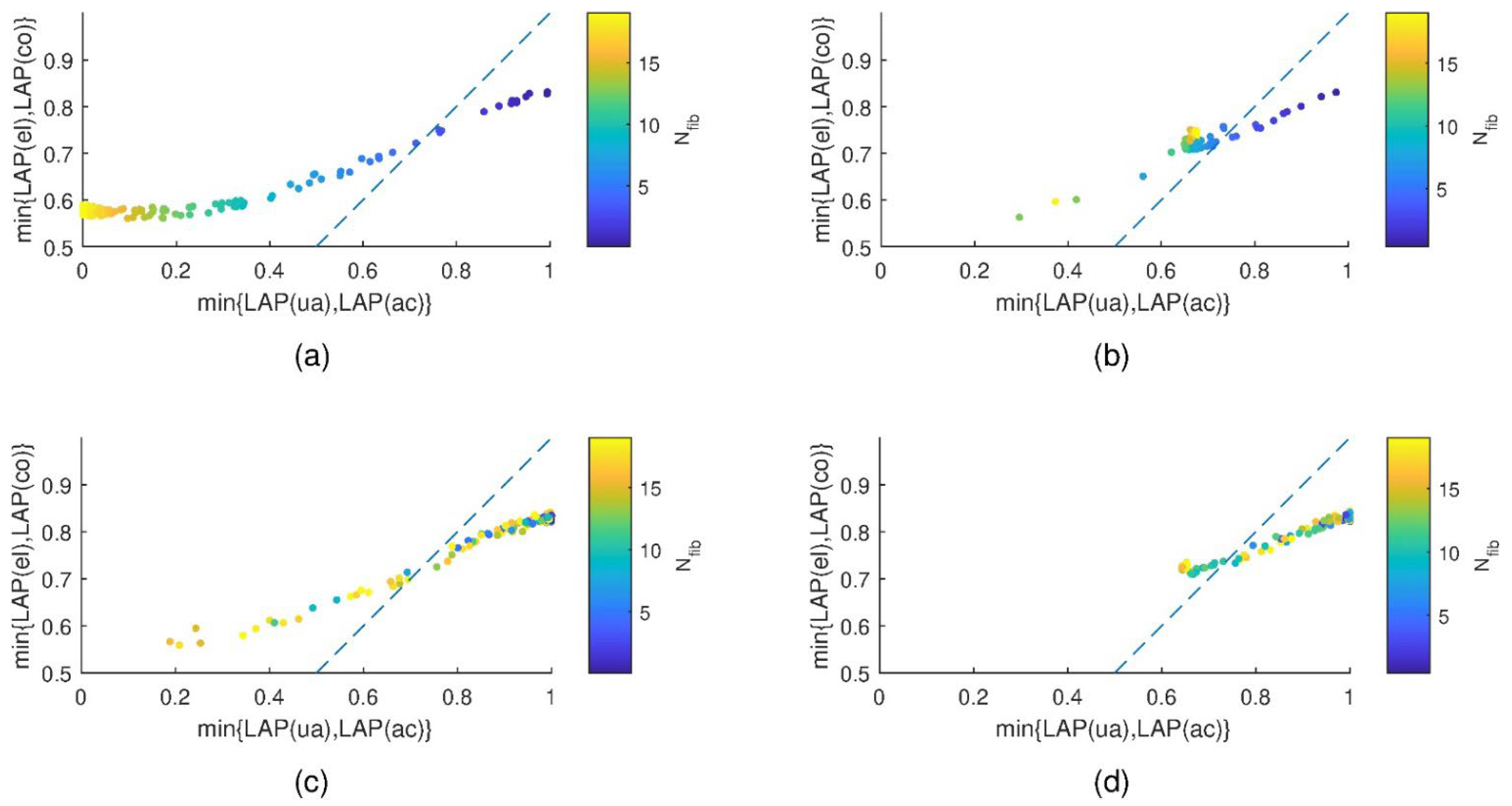
Figure 13 shows scatter plots of the minimum LAP score achieved with and without implantation. The dashed lines are the lines of equality. The number of functional synapses per IHC is color-coded. Each dot reflects one subject. Only subjects with CS are reported. The plots show distinct types of hearing loss, i.e., (a) CS, (b) CGL + CS, (c) IHCL + CS, and (d) CGL + IHCL + CS. A relationship between the degree of CS and the position across the coordinate systems was observed. In particular, subjects with mild CS, i.e., higher number of fibers, tended to lie on the left side of the line of equality, and vice versa. This trend appears to be fuzzier with IHCL (bottom row), as some subjects with low CS were located to the right of the line of equality. These were supposedly subjects with severe IHCL. As in Figure 12, two distinct patterns were observed in the plots with and without CGL.

In contrast to what was observed for IHCL and CS, no clear relationship between the degree of CS and the position across the coordinate system was observed (not shown here).

3.4. Implantation Recommendations Based on Multiple Hearing Loss Parameters

Table 2. Logistic regression coefficients for predicting cochlear implantation recommendation from hearing loss parameters $\mathsf{\Psi }$.

		Model Coefficients	p-Value
	Intercept	4.875	<0.001
Hearing loss parameters	${\mathrm{I}}_{\mathrm{f}}$ (dB)	2.417	<0.001
	${\mathrm{I}}_{\mathrm{s}}$ (dB)	−0.053	0.079
	${\mathrm{O}}_{\mathrm{f}}$ (dB)	−0.098	0.161
	${\mathrm{O}}_{\mathrm{s}}$ (dB)	0.175	0.007
	${\mathrm{N}}_{\mathrm{fib}}$	−1.754	<0.001

The parameters were the flat and sloping components of the loss of inner hair cells (${\mathrm{I}}_{\mathrm{f}}$ and ${\mathrm{I}}_{\mathrm{s}}$), the flat and sloping components of the cochlear gain loss (${\mathrm{O}}_{\mathrm{f}}$ and ${\mathrm{O}}_{\mathrm{s}}$), and the number of active fibers per IHC (${\mathrm{N}}_{\mathrm{fib}}$), reflecting cochlear synaptopathy.

lists the model coefficients and p-values for the logistic regression. The coefficients may be interpreted as follows: Three hearing loss parameters showed significant effects. First, a 1 dB increase in ${\mathrm{I}}_{\mathrm{f}}$ increased the odds for a CI recommendation by a factor of exp(2.417). Second, the loss of one synapse per IHC increased the odds by a factor of exp(1.754). Finally, a 1 dB increase in ${\mathrm{O}}_{\mathrm{s}}$ increased the odds by a factor of exp(0.175). The coefficients of the other hearing loss parameters were non-significant.

Table 3. Confusion table of the logistic regression.

		True Class
		Implant	No Implant
Predicted class	Implant	436	6
	No Implant	7	575

The true class refers to the class predicted by the simulation, i.e., whether a hearing prosthesis option involving cochlear implantation has the minimum LAP. The predicted class refers to the prediction made by the logistic regression.

reports the confusion table of logistic regression, for which the hearing loss parameters were used as predictors. The true class (‘implant’ versus ‘no implant’) refers to the recommendation based on the minimum LAP obtained by the simulation. The predicted class refers to the output of the logistic regression. The numbers observed in the confusion table reflect excellent classification performance, since the implantation recommendation of the vast majority of the subjects is correctly predicted by the logistic regression.

Table 4. Test statistics and confidence intervals regarding the logistic regression.

Statistic	Value	95% Confidence Interval
Sensitivity	98.19%	96.47% to 99.22%
Specificity	98.62%	97.30% to 99.40%
Positive likelihood ratio	71.31	35.83 to 141.94
Negative likelihood ratio	0.02	0.01 to 0.04
Positive predictive value	98.19%	96.47% to 99.08%
Negative predictive value	98.62%	97.30% to 99.30%
Accuracy	98.44%	97.47% to 99.10%

lists test statistics for the logistic regression. All the listed numbers reflect exceptionally high performance, since the sensitivity, the specificity, the positive and negative predictive values, and the accuracy estimates all exceeded 98%, and the positive and negative likelihood ratios were large and small, respectively.

Table 5. Confusion table of the support vector machine classification using a quadratic kernel.

		True Class
		Implant	No Implant
Predicted class	Implant	576	5
	No Implant	3	440

The true class refers to the class predicted by the simulation, i.e., whether a hearing prosthesis option involving cochlear implantation has the minimum LAP. The predicted class refers to the prediction made by the support vector machine.

reports the confusion table of the support vector machine, for which the hearing loss parameters were used as predictors. The numbers observed in the confusion table reflect excellent classification performance, which was even slightly better than the performance observed for logistic regression.

Table 6. Test statistics and confidence intervals regarding the support vector machine classification using a quadratic kernel.

Statistic	Value	95% Confidence Interval
Sensitivity	99.48%	98.49% to 99.89%
Specificity	98.88%	97.40% to 99.63%
Positive likelihood ratio	88.54	37.03 to 211.68
Negative likelihood ratio	0.01	0.00 to 0.02
Positive predictive value	99.14%	97.97% to 99.64%
Negative predictive value	99.32%	97.94% to 99.78%
Accuracy	99.22%	98.47% to 99.66%

lists test statistics for the support vector machine. The small improvement as compared to logistic regression may have been due to the support vector machine’s capability to model interactions between hearing loss parameters, enabled by the use of a quadratic kernel.

4. Discussion

A simulation study on place–time representations of AN firing rates predicted for different hearing prostheses options and types and degrees of hearing loss was conducted. The prosthesis options were as follows: unaided hearing, acoustic amplification, electrical stimulation, and electrical stimulation combined with acoustic amplification. The hearing loss types were IHCL, CGL, and CS. The firing rates of the individual prosthesis options were compared to NH reference firing rates. Finding the minimum LAP of the AN firing rates served two purposes. First, the fitting parameters of the hearing prostheses were optimized, and second, personalized hearing prosthesis recommendations were obtained. The distinction between the groups ‘implant’ and ‘no implant’ is clinically highly relevant. The former group includes subjects for which the prosthesis recommendation involves electrical stimulations. It was found that loss of IHCs was most influential to the ‘implant’/‘no implant’ distinction, followed by CS. The ‘implant’ group included subjects with a substantial number of damaged IHCs and subjects with severe CS. The estimated threshold of IHCL appeared to be remarkably low as compared to available clinical guidelines that basically suggest implantation for severe or profound hearing loss only. However, it should be noted that ${\mathrm{I}}_{\mathrm{f}}$ and ${\mathrm{I}}_{\mathrm{s}}$ are not directly comparable to dB HL because they rather refer to spatial density of functional IHCs instead of sound pressure levels. The damage of OHCs appears to influence the implantation recommendation only slightly. Moreover, the distinction between frequency-flat and frequency-sloping components appears to be of limited relevance to the recommendation.

Several clinical guidelines regarding the indication of cochlear implantation are reviewed hereafter. In summary, cochlear implantation is indicated for severe to profound hearing loss, which may include individuals with significant residual hearing. For example, Leigh et al. found that cochlear-implanted children perform significantly better in speech recognition than their peers with profound hearing loss, i.e., with pure tone average thresholds exceeding 90 dB HL, when using acoustical amplification [26]. However, multiple factors need to be taken into account, including subjects’ experience with acoustic amplification; unaided air and bone conduction hearing thresholds; auditory speech recognition; and non-behavioral audiological function such as optoacoustic emissions, immittance testing, and auditory brainstem responses [27].

The recent guideline published by the National Institute for Health and Care Excellence (NICE) suggests that subjects with pure tone thresholds of 80 dB HL or greater at two or more frequencies between 500 Hz and 4 kHz are eligible for cochlear implantation if they do not benefit sufficiently from acoustic amplification [28]. The latter requires for adults a phoneme score of 50% or greater in the Arthur Boothroyd word test presented at 70 dB (A), and for children speech language and listening skills that are appropriate for their age, developmental stage, and cognitive abilities. A comprehensive and recent summary of evidence regarding CI candidacy criteria is provided in [27]. The Western Australian Department of Health lists selection criteria for cochlear implantation as (i) moderately severe to profound bilateral sensorineural hearing loss, (ii) little or no benefit from acoustic amplification, (iii) open-set sentence scores in quiet in the worse ear <65% and in the better ear <85%, (iv) open-set phoneme scores in quiet in the worse ear <45% and in the better ear <65% with no radiological or medical contraindications, (v) appropriate expectations and commitment from client and family, and (vi) motivation of the client [29].

The most recent practice policy for cochlear implantation of the American Speech-Language-Hearing Association (ASHA) was published in 2004 [30]. This policy permits cochlear implantation in subjects 2 years and older if pure tone average thresholds are at 70 dB HL or greater, and in children younger than 2 years of pure tone average thresholds are at 90 dB HL or greater. For adults, cochlear implantation is permitted for open-set sentence recognition scores of up to approximately 50 to 60%. A question central to the indication of cochlear implantation is “Is it likely that an individual will receive more communication benefit from a CI than from a hearing aid or, alternatively, from no hearing prosthesis at all?” [30].

Moreover, commercial manufacturers such as MED-EL and Cochlear Ltd. provide criteria for indicating cochlear implantation [31,32]. In the report by MED-EL, slightly diverging implantation criteria are listed for a few countries, i.e., Germany, the United Kingdom, France, (Western) Australia, the Kingdom of Saudi Arabia, and the Republic of Korea. Examples of threshold hearing levels eligible for cochlear implantation range up to 70 dB HL, which may mark the borderline between moderate and severe hearing loss. Cochlear Ltd. even indicates on their website cochlear implantation at low-frequency threshold hearing levels of up to 40 dB HL [31].

Besides hearing thresholds, also subjects’ and families’ preferences, motivation, commitment, appropriateness of expectation, and other psychological aspects as well as aspects of quality of life play a role, and assessment differs for adults and children. In particular, a patients’ hearing must be assessed in a holistic way instead of only applying strict criteria, which may turn the decision for a significant subset of individuals of the candidacy population [33]. To address some of these factors, the ‘costs’ of acoustic amplification ${\mathsf{\lambda }}_{\mathrm{amp}}$ and cochlear implantation ${\mathsf{\lambda }}_{\mathrm{imp}}$ that we proposed to be included in the decision process may be adjusted. These cost factors may be understood as means for assessing the relative weightings of burdens, costs, and risks of using a hearing aid and or cochlear implantation. A similar strategy was proposed in a broader context to assess patient preferences on clinical interventions in the past [34]. We saw that thresholds of IHCL indicating cochlear implantation varied considerably when the penalty parameters were varied.

An added value of the presented study over current practical guidelines arises from the synergy between the state-of-the-art modelling approaches that were combined for the purpose of comparing available hearing prostheses options in a personalized way. For example, one may want to predict in clinically doubtful scenarios whether hearing performance is likely to improve when a CI is used, and how large the risk of a performance decrease may be. To the best of the author’s knowledge the presented study is the first that proposes such a modelling approach for the purpose of working towards a non-black box decision support system for the clinical care of hearing impairment. While a holistic understanding of a patient’s situation is important, the proposed modelling approach may be seminal for future studies that aim at establishing a physiologically grounded decision support.

Limitations of the study and suggestions for future work include the following: First, for the fitting of the CIs, only the insertion depth of the electrode was used as a fitting parameter, and only the CIS strategy was used. The choice of only optimizing the insertion depth was based on unpublished preliminary experimentation during which the largest variance of the LAP was observed when insertion depths were varied, whereas only little variance of LAP was observed for parameters of frequency and level mapping. Moreover, different surgical approaches exist and may influence the outcome [35]. Thus, suggestions for future research include having a closer look at the remaining fitting parameters of the CI, and to test different stimulation strategies than only CIS, such as the Advanced Combination Encoder (ACE) [36], specialized strategies for optogenetic stimulation [37], Stimulation based on Auditory Modelling (SAM) [38], or others [25].

Second, only root mean squared differences of AN firing rates were used for fitting and comparison. This choice neglects the plasticity of human central auditory processing, which enables impaired listeners to accommodate to impaired hearing to some degree [39]. An advanced objective for fitting and comparison instead of the LAP may be developed in the future with the aim of reflecting human ability to accommodate. An argument in favor of direct comparison of AN firing rates is that a proposal exists in which an electrical stimulation strategy aims at mimicking AN firing patterns of NH [38]. Moreover, a pursuit towards near physiological spectral selectivity is being observed [37]. Thus, we assume that hearing rehabilitation is more straightforward if recovered AN firing patterns are similar to natural ones. We also experimented using the structural similarity index (SSIM) instead of the LAP [40]. Results obtained using the SSIM, which is a measure for visual image similarity, are similar to results obtained with the LAP.

Third, the hearing loss parameters used in our study are not easily transferable into hearing threshold levels versus frequency, i.e., pure tone audiograms, which limits the comparability of our results with existing clinical guidelines. In fact, CGL was reported to result in hearing threshold levels of up to 60 dB [9], while the CGL parameters of the used model result in complete loss of cochlear gain as soon as the hearing thresholds are elevated by 35 dB only [8]. Moreover, our parameters indicating IHCL reflect spatial density of functional IHCs and are not meant to directly correspond to hearing threshold levels. In the future, we suggest continuing with estimating cochlear parameters using audiometric methods. Evaluation of otoacoustic emissions, in particular transient-evoked otoacoustic emissions (TEOAEs) and distortion production otoacoustic emissions (DPOAEs), as well as the evaluation of cochlear microphonics (CMs), may enable the estimation of CGL parameters. Estimation of IHCL parameters may be enabled by additional evaluation of the compound action potential (CAP) obtained with invasive or non-invasive electrocochleography (ECochG), which is similar to Wave-I of the auditory brainstem response (ABR) but has a better signal-to-noise-ratio. Moreover, dead regions may be identified by the TEN(HL) test [41]. Personalized outer and middle ear filters may be obtained from measuring head-related transfer functions, and from tympanometry. A suggestion for the validation of the presented simulation study would be to obtain pre- and post-implantation measurements for patients and dichotomize them into groups of subjects with favorable and unfavorable implantation outcome. One may hypothesize that the proposed simulation may help to predict before implantation which of the individuals benefit from implantation.

Finally, only monaural processing of a close-mic signal was simulated, which does not enable the studying of the human ability to externalize and localize sound (e.g., in CIs, [42]), limiting the possibilities of studying auditory stream segregation, e.g., such as in the cocktail party effect [43,44,45,46]. In particular, difficulties of CI users in adverse listening conditions [47,48] may be considered in the future.

5. Conclusions

The suggested conclusions are the following. First, cochlear implantation appears to be indicated for individuals with more than approximately two-thirds of IHCs damaged. Second, the same applies to individuals with CS when more than an average of approximately 12 synapses per IHC are damaged. Third, CGL and frequency profiles of damages of hair cells appear to influence the indication of cochlear implantation only slightly in the presented simulations.

References

- Ruben, R.J. Redefining the Survival of the Fittest: Communication Disorders in the 21st Century. Laryngoscope 2000, 110, 241–245. [Google Scholar] [CrossRef] [PubMed]
- Feder, K.; Michaud, D.; Ramage-Morin, P.; McNamee, J.; Beauregard, Y. Prevalence of Hearing Loss among Canadians Aged 20 to 79: Audiometric Results from the 2012/2013 Canadian Health Measures Survey. Health Rep. 2015, 26, 18–25. [Google Scholar] [PubMed]
- Moser, T.; Predoehl, F.; Starr, A. Review of Hair Cell Synapse Defects in Sensorineural Hearing Impairment. Otol. Neurotol. 2013, 34, 995–1004. [Google Scholar] [CrossRef] [PubMed] [Green Version]
- Kujawa, S.G.; Liberman, M. Synaptopathy in the Noise-Exposed and Aging Cochlea: Primary Neural Degeneration in Acquired Sensorineural Hearing Loss. Hear. Res. 2015, 330, 191–199. [Google Scholar] [CrossRef] [Green Version]
- Liberman, M.; Epstein, M.J.; Cleveland, S.S.; Wang, H.; Maison, S.F. Toward a Differential Diagnosis of Hidden Hearing Loss in Humans. PLoS ONE 2016, 11, e0162726. [Google Scholar] [CrossRef]
- Liberman, M.; Kujawa, S.G. Cochlear Synaptopathy in Acquired Sensorineural Hearing Loss: Manifestations and Mechanisms. Hear. Res. 2017, 349, 138–147. [Google Scholar] [CrossRef]
- Carney, L.H. Supra-Threshold Hearing and Fluctuation Profiles: Implications for Sensorineural and Hidden Hearing Loss. JARO J. Assoc. Res. Otolaryngol. 2018, 19, 331–352. [Google Scholar] [CrossRef]
- Verhulst, S.; Altoè, A.; Vasilkov, V. Computational Modeling of the Human Auditory Periphery: Auditory-Nerve Responses, Evoked Potentials and Hearing Loss. Hear. Res. 2018, 360, 55–75. [Google Scholar] [CrossRef]
- Moore, B. Cochlear Hearing Loss: Physiological, Psychological and Technical Issues; John Wiley & Sons, Ltd.: West Sussex, UK, 2007; ISBN 9780470516331. [Google Scholar]
- Boisvert, I.; Reis, M.; Au, A.; Cowan, R.; Dowell, R.C. Cochlear Implantation Outcomes in Adults: A Scoping Review. PLoS ONE 2020, 15, e0232421. [Google Scholar] [CrossRef]
- Wilson, B.S.; Dorman, M.F. Cochlear Implants: A Remarkable Past and a Brilliant Future. Hear. Res. 2008, 242, 3–21. [Google Scholar] [CrossRef] [Green Version]
- Verhulst, S.; Altoè, A.; Vasilkov, V. Verhulst et al.’s Model Code. Available online: https://github.com/HearingTechnology/Verhulstetal2018Model (accessed on 19 September 2019).
- Fredelake, S.; Hohmann, V. Factors Affecting Predicted Speech Intelligibility with Cochlear Implants in an Auditory Model for Electrical Stimulation. Hear. Res. 2012, 287, 76–90. [Google Scholar] [CrossRef] [PubMed]
- Hamacher, V. Signalverarbeitungsmodelle Des Elektrisch Stimulierten Gehörs, Rheinisch-Westfälischen Technischen Hochschule Aachen; Hochschule: Aachen, Germany, 2004. [Google Scholar]
- Grimm, G.; Herzke, T.; Ewert, S.; Hohmann, V. Implementation and Evaluation of an Experimental Hearing Aid Dynamic Range Compressor Gain Prescription. In Proceedings of the DAGA, Nürnberg, Germany, 16–19 March 2015; pp. 996–999. [Google Scholar]
- Herzke, T.; Kayser, H.; Loshaj, F.; Grimm, G.; Hohmann, V. Open Signal Processing Software Platform for Hearing Aid Research (OpenMHA). In Proceedings of the Linux Audio Conference, Saint-Étienne, France, 1–7 July 2017; pp. 35–42. [Google Scholar]
- Chan, W.X.; Yoon, Y.J.; Shin, C.S.; Kim, N. Mechanical Effects of Cochlear Implant on Acoustic Hearing. IEEE Trans. Biomed. Eng. 2019, 66, 1609–1617. [Google Scholar] [CrossRef] [PubMed]
- Elliott, S.J.; Ni, G.; Verschuur, C.A. Modelling the Effect of Round Window Stiffness on Residual Hearing after Cochlear Implantation. Hear. Res. 2016, 341, 155–167. [Google Scholar] [CrossRef]
- Puria, S. Measurements of Human Middle Ear Forward and Reverse Acoustics: Implications for Otoacoustic Emissions. J. Acoust. Soc. Am. 2003, 113, 2773–2789. [Google Scholar] [CrossRef] [PubMed]
- Shera, C.; Zweig, G. A Symmetry Suppresses the Cochlear Catastrophe. J. Acoust. Soc. Am. 1991, 89, 1276–1289. [Google Scholar] [CrossRef] [PubMed]
- Altoè, A.; Pulkki, V.; Verhulst, S. The Effects of the Activation of the Inner-Hair-Cell Basolateral K + Channels on Auditory Nerve Responses. Hear. Res. 2018, 364, 68–80. [Google Scholar] [CrossRef]
- Liberman, M. Auditory-Nerve Response from Cats Raised in a Low-Noise Chamber. J. Acoust. Soc. Am. 1978, 63, 442–455. [Google Scholar] [CrossRef]
- Westerman, L.A.; Smith, R.L. A Diffusion Model of the Transient Response of the Cochlear Inner Hair Cell Synapse. J. Acoust. Soc. Am. 1988, 83, 2266–2276. [Google Scholar] [CrossRef]
- Peterson, A.J.; Irvine, D.R.F.; Heil, P. A Model of Synaptic Vesicle-Pool Depletion and Replenishment Can Account for the Interspike Interval Distributions and Nonrenewal Properties of Spontaneous Spike Trains of Auditory-Nerve Fibers. J. Neurosci. 2014, 34, 15097–15109. [Google Scholar] [CrossRef] [Green Version]
- Wilson, B.S. Getting a Decent (but Sparse) Signal to the Brain for Users of Cochlear Implants. Hear. Res. 2015, 322, 24–38. [Google Scholar] [CrossRef] [Green Version]
- Leigh, J.; Dettman, S.; Dowell, R.; Sarant, J. Evidence-Based Approach for Making Cochlear Implant Recommendations for Infants with Residual Hearing. Ear Hear. 2011, 32, 313–322. [Google Scholar] [CrossRef] [PubMed]
- Messersmith, J.J.; Entwisle, L.; Warren, S.; Scott, M. Clinical Practice Guidelines: Cochlear Implants. J. Am. Acad. Audiol. 2019, 30, 827–844. [Google Scholar] [CrossRef] [PubMed]
- Trowman, R.; Garrett, Z.; Dent, R.; Saile, E.; Powell, J. Cochlear Implants for Children and Adults with Severe to Profound Deafness; (Technical Appraisal 566); National Institute for Health and Care Excellence (NICE): London, UK; Manchester, UK, 2019. [Google Scholar]
- Upson, G.; Rodrigues, S.; Chester-Browne, R.; Sucher, C.; Robertson, B.; Atlas, M. Clinical Guidelines for Adult Cochlear Implantation; Government of Western Australia, Department of Health: Perth, WA, Australia, 2012.
- American Speech-Language-Hearing Association. Cochlear Implants; [Technical Report]; American Speech-Language-Hearing Association: Rockville, MD, USA, 2004. [Google Scholar]
- MED-EL. Who Gets a Cochlear Implant; [Special Report No. 3]; MED-EL: Innsbruck, Austria, 2014. [Google Scholar]
- Cochlear Ltd. Cochlear Implant Candidacy Information. Available online: https://www.cochlear.com/us/en/professionals/products/cochlear-implants/candidacy (accessed on 24 September 2020).
- Hanvey, K.; Ambler, M.; Maggs, J.; Wilson, K. Criteria versus Guidelines: Are We Doing the Best for Our Paediatric Patients? Cochlear Implant. Int. 2016, 17, 78–82. [Google Scholar] [CrossRef] [PubMed] [Green Version]
- Dollaghan, C. The Handbook for Evidence-Based Practice in Communication Disorders; Paul H. Brookes: Baltimore, MD, USA, 2007; ISBN 9781557668707. [Google Scholar]
- Freni, F.; Gazia, F.; Slavutsky, V.; Scherdel, E.P.; Nicenboim, L.; Posada, R.; Portelli, D.; Galletti, B.; Galletti, F. Cochlear Implant Surgery: Endomeatal Approach versus Posterior Tympanotomy. Int. J. Environ. Res. Public Health 2020, 17, 4187. [Google Scholar] [CrossRef]
- Saba, J.; Ali, H.; Hansen, J. Formant Priority Channel Selection for an “n -of- m” Sound Processing Strategy for Cochlear Implants. J. Acoust. Soc. Am. 2018, 144, 3371–3380. [Google Scholar] [CrossRef]
- Dieter, A.; Duque-Afonso, C.J.; Rankovic, V.; Jeschke, M.; Moser, T. Near Physiological Spectral Selectivity of Cochlear Optogenetics. Nat. Commun. 2019, 10, 1962. [Google Scholar] [CrossRef]
- Harczos, T.; Chilian, A.; Husar, P. Making Use of Auditory Models for Better Mimicking of Normal Hearing Processes with Cochlear Implants: The SAM Coding Strategy. IEEE Trans. Biomed. Circuits Syst. 2013, 7, 414–425. [Google Scholar] [CrossRef]
- Salvi, R.; Sun, W.; Ding, D.; Di Chen, G.; Lobarinas, E.; Wang, J.; Radziwon, K.; Auerbach, B.D. Inner Hair Cell Loss Disrupts Hearing and Cochlear Function Leading to Sensory Deprivation and Enhanced Central Auditory Gain. Front. Neurosci. 2017, 10, 621. [Google Scholar] [CrossRef] [Green Version]
- Wang, Z.; Bovik, A.C.; Sheikh, H.R.; Simoncelli, E.P. Image Quality Assessment: From Error Visibility to Structural Similarity. IEEE Trans. Image Process. 2004, 13, 600–612. [Google Scholar] [CrossRef] [Green Version]
- Moore, B. Testing for Cochlear Dead Regions: Audiometer Implementation of the TEN(HL) Test. Hear. Rev. 2010, 17, 10–16, 48. [Google Scholar]
- Majdak, P.; Goupell, M.J.; Laback, B. Two-Dimensional Localization of Virtual Sound Sources in Cochlear-Implant Listeners. Ear Hear. 2011, 32, 198–208. [Google Scholar] [CrossRef] [PubMed] [Green Version]
- Baumgärtel, R.M.; Hu, H.; Kollmeier, B.; Dietz, M. Extent of Lateralization at Large Interaural Time Differences in Simulated Electric Hearing and Bilateral Cochlear Implant Users. J. Acoust. Soc. Am. 2017, 141, 2338–2352. [Google Scholar] [CrossRef] [PubMed]
- Kan, A.; Jones, H.G.; Litovsky, R.Y. Lateralization of Interaural Timing Differences with Multi-Electrode Stimulation in Bilateral Cochlear-Implant Users. J. Acoust. Soc. Am. 2016, 140, EL392–EL398. [Google Scholar] [CrossRef] [PubMed] [Green Version]
- Hu, H.; Ewert, S.; McAlpine, D.; Dietz, M. Differences in the Temporal Course of Interaural Time Difference Sensitivity between Acoustic and Electric Hearing in Amplitude Modulated Stimuli. J. Acoust. Soc. Am. 2017, 141, 1862–1873. [Google Scholar] [CrossRef] [PubMed]
- Best, V.; Laback, B.; Majdak, P. Binaural Interference in Bilateral Cochlear-Implant Listeners. J. Acoust. Soc. Am. 2011, 130, 2939–2950. [Google Scholar] [CrossRef]
- Prejban, D.A.; Hamzavi, J.-S.; Arnoldner, C.; Liepins, R.; Honeder, C.; Kaider, A.; Gstöttner, W.; Baumgartner, W.-D.; Riss, D. Single Sided Deaf Cochlear Implant Users in the Difficult Listening Situation: Speech Perception and Subjective Benefit. Otol. Neurotol. 2018, 39, e803–e809. [Google Scholar] [CrossRef] [PubMed]
- Koning, R.; Wouters, J. Speech Onset Enhancement Improves Intelligibility in Adverse Listening Conditions for Cochlear Implant Users. Hear. Res. 2016, 342, 13–22. [Google Scholar] [CrossRef]
Figure 1.
Overview of the modelling approach to predict AN firing rates for different hearing prosthesis options in a personalized way, as well as to obtain the LAP scores for each prosthesis option. The stimulus s(t) is put into models of acoustical stimulation, acoustical amplification, and electrical stimulation to obtain place–time representations of AN firing rates. Firing rates are obtained for the normal hearing reference (nh), unaided hearing (ua), electrical stimulation including residual acoustical hearing (el), sole acoustical amplification (ac), and electrical stimulation combined with acoustical amplification (co). The loss of action potentials (LAP) is obtained for ua, el, ac, and co, by comparing the corresponding AN firing rates with nh. * For modelling low-frequency residual hearing with a cochlear implant, a 20 dB attenuation is applied to the stimulus.
Figure 2.
Numbers of subjects with regard to the individually predicted best hearing prosthesis, i.e., the prosthesis corresponding to the minimum cost-adjusted loss of action potentials (LAP) score. The types of hearing loss are as follows: (a) normal hearing (NH), (b) cochlear gain loss (CGL), (c) loss of IHCs (IHCL), (d) IHCL + CGL. The types of hearing prosthesis are as follows: unaided hearing (ua), acoustical amplification (ac), electrical stimulation (el), and el combined with ac (co).
Figure 3.
Numbers of subjects with regard to the individually predicted best hearing prosthesis, i.e., the prosthesis corresponding to the minimum cost-adjusted loss of action potentials (LAP) score. The types of hearing loss are as follows: (a) cochlear synaptopathy (CS), (b) cochlear gain loss (CGL) + CS, (c) loss of IHCs (IHCL) + CGL + CS, (d) IHCL + CGL + CS. The types of hearing prosthesis are as follows: unaided hearing (ua), acoustical amplification (ac), electrical stimulation (el), and el combined with ac (co).
Figure 4.
AN firing rates with regard to fiber index and time. The subject has severe IHCL and CGL. The stimulus was an audio recording of a speaker uttering the word ‘nest’, which was scaled to an equivalent sound pressure level of 65 dB (20 µPa). (a) Normal hearing reference. (b) Unaided hearing, with hearing loss parameters (, , , , and ). (c) Sole acoustical amplification, with amplification parameters ( and ). (d) Sole electrical stimulation, with insertion depth of the CI. (e) Electrical stimulation combined with acoustic amplification, with insertion depth of the CI and amplification parameter . LAP refers to the cost-adjusted loss of action potentials.
Figure 5.
AN firing rates with regard to fiber index and time. The subject showed moderate IHCL at low frequencies and severe IHCL at high frequencies. (a) Normal hearing reference. (b) Unaided hearing, with hearing loss parameters (, , , , and ). (c) Sole acoustical amplification, with amplification parameters ( and ). (d) Sole electrical stimulation, with insertion depth of the CI. (e) Electrical stimulation combined with acoustic amplification, with insertion depth of the CI and amplification parameter . LAP refers to the cost-adjusted loss of action potentials.
Figure 6.
AN firing rates with regard to fiber index and time. The subject showed moderate CGL. See (a) Normal hearing reference. (b) Unaided hearing, with hearing loss parameters (, , , , and ). (c) Sole acoustical amplification, with amplification parameters ( and ). (d) Sole electrical stimulation, with insertion depth of the CI. (e) Electrical stimulation combined with acoustic amplification, with insertion depth of the CI and amplification parameter . LAP refers to the cost-adjusted loss of action potentials.
Figure 7.
AN firing rates with regard to fiber index and time. The subject showed moderate to severe CS. (a) Normal hearing reference. (b) Unaided hearing, with hearing loss parameters (, , , , and ). (c) Sole acoustical amplification, with amplification parameters ( and ). (d) Sole electrical stimulation, with insertion depth of the CI. (e) Electrical stimulation combined with acoustic amplification, with insertion depth of the CI and amplification parameter . LAP refers to the cost-adjusted loss of action potentials.
Figure 8.
Bar charts of the cost-adjusted loss of action potentials (LAP). Four cases selected for detailed analysis, i.e., the cases reported in Figure 4, Figure 5, Figure 6 and Figure 7. The bar charts (a–d) reflect for each of the four subjects personalized predictions of LAP with regard to the hearing prosthesis options. The shortest bars in each of (a–d) reflect the recommended hearing prosthesis option. Their colors are made distinct. The bar charts may be displayed to clinicians as personalized recommendation charts. They provide a concise overview of the prosthesis options, enabling quick judgement of absolute and relative bar heights. Unaided hearing (ua), sole acoustical amplification (ac), sole electrical stimulation (el), and electric stimulation combined with acoustical amplification (co).
Figure 9.
Hearing loss parameters with regard to implantation recommendation. Shown are (a) the flat and (b) sloping components of the loss of IHCs, i.e., and ; (c) the flat and (d) sloping components of the cochlear gain loss, i.e., and ; and (e) the average number of active fibers per IHC , reflecting cochlear synaptopathy.
Figure 10.
ROC curves regarding binary prediction of implantation recommendation. The used single predictors are as follows: (a) the flat component of the IHC loss (), (b) the sloping component of the IHC loss (), (c) the flat component of the cochlear gain loss (), (d) the sloping component of the cochlear gain loss (), and (e) the number of active fibers attached to each IHC (). Yellow asterisks and cut-off thresholds THR were obtained at maximal perpendicular distances of the ROC curves to the lines of equality.
Figure 11.
Cut-off threshold THR of the flat component of the loss of inner hair cells (dB), with respect to the amplification cost and implantation cost . One operating point (yellow asterisks) was at , and , the other one was at .
Figure 12.
Minimum LAP achieved with (y-axes) and without (x-axes) implantation. The dashed lines are the lines of equality. The flat component of IHCL is color-coded. The shown types of hearing losses are as follows: (a) IHCL only, (b) CGL and IHCL, (c) IHCL + CS, and (d) CGL + IHCL + CS.
Figure 13.
Minimum LAP achieved with (y-axes) and without (x-axes) implantation. The dashed lines are the lines of equality. The number of functional synapses per IHC is color-coded. The shown types of hearing losses are as follows: (a) CS only, (b) CGL + CS, (c) IHCL + CS, and (d) CGL + IHCL + CS.