
Auto-Detection of Hidden Corrosion in an Aircraft Structure by Electromagnetic Testing: A Machine-Learning Approach


Abstract
:1. Introduction
2. Electromagnetic Testing Principle
3. Data Preparation
3.1. Experimental Setup
3.2. Data Preparation
4. Machine Learning Algorithms
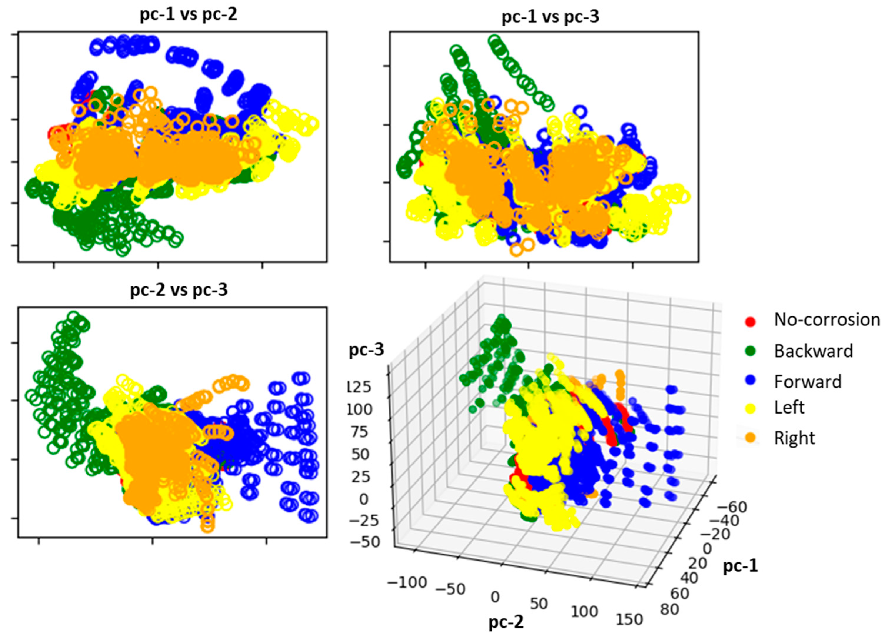
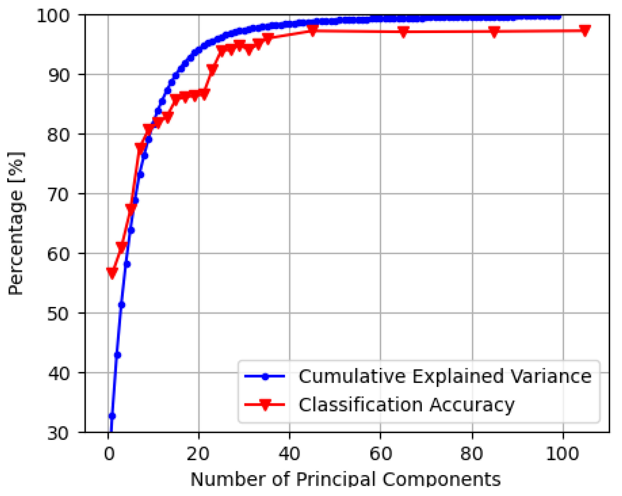
4.1. Principal Component Analysis (PCA)
4.2. Support Vector Machine (SVM)
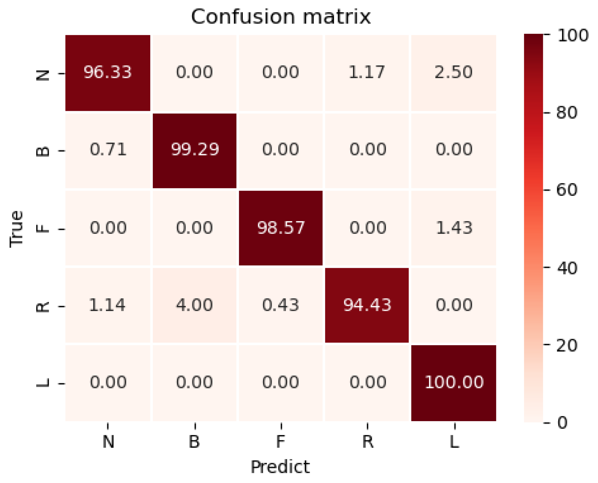
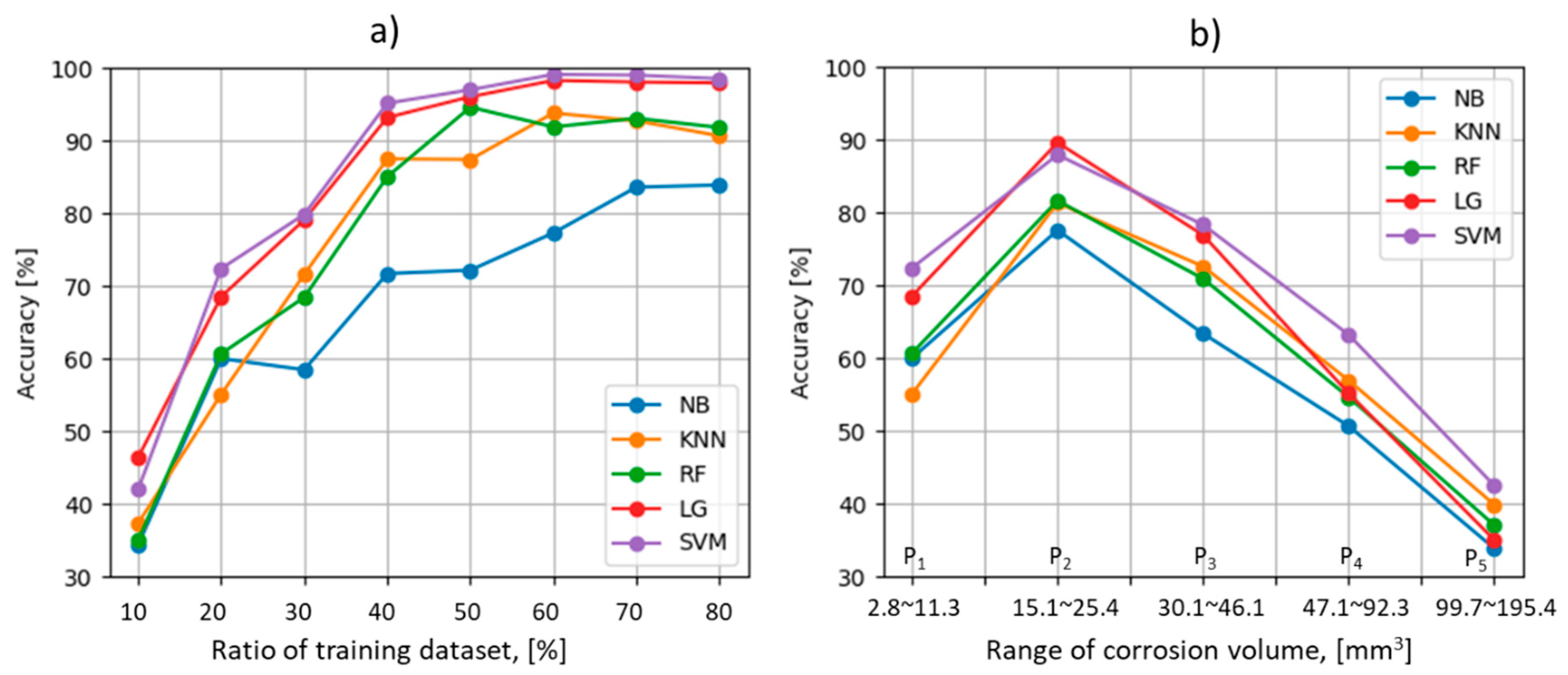
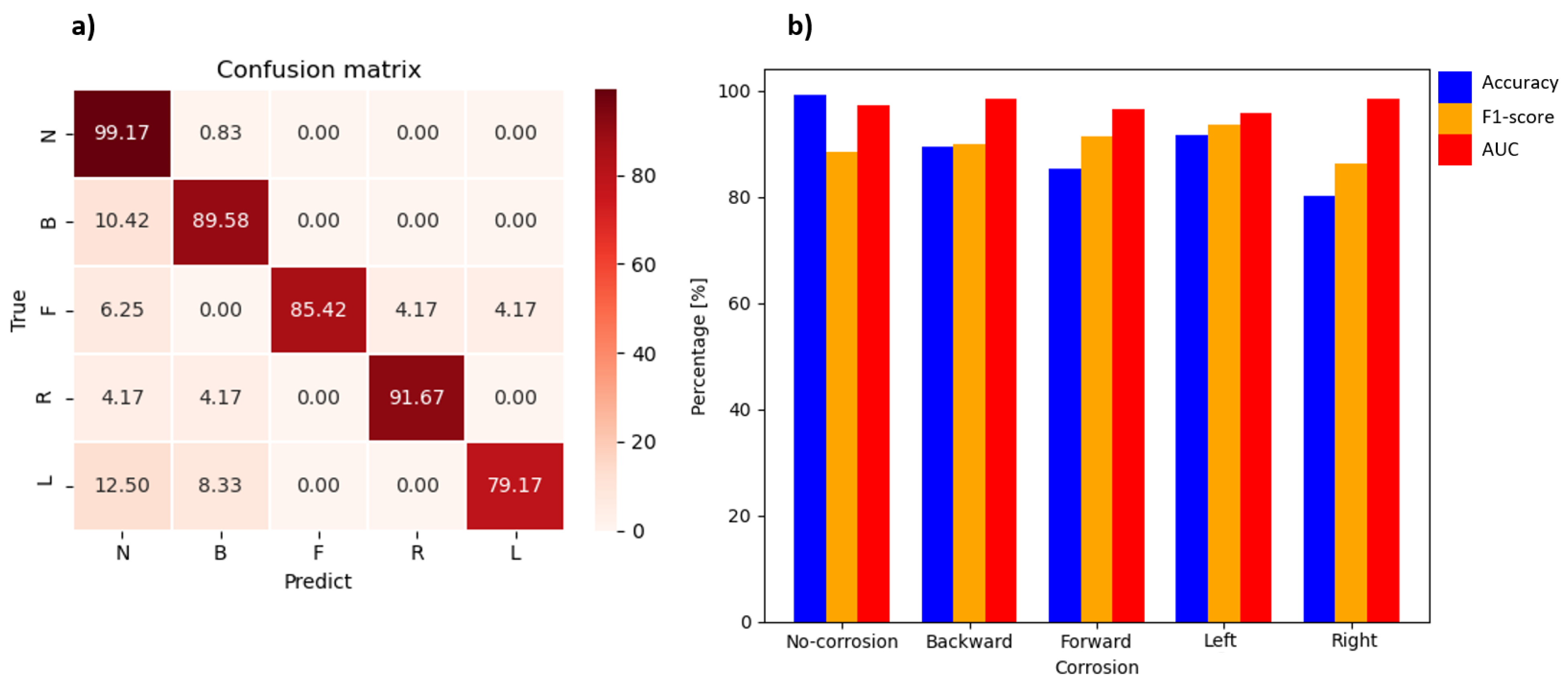
4.3. Classification Results
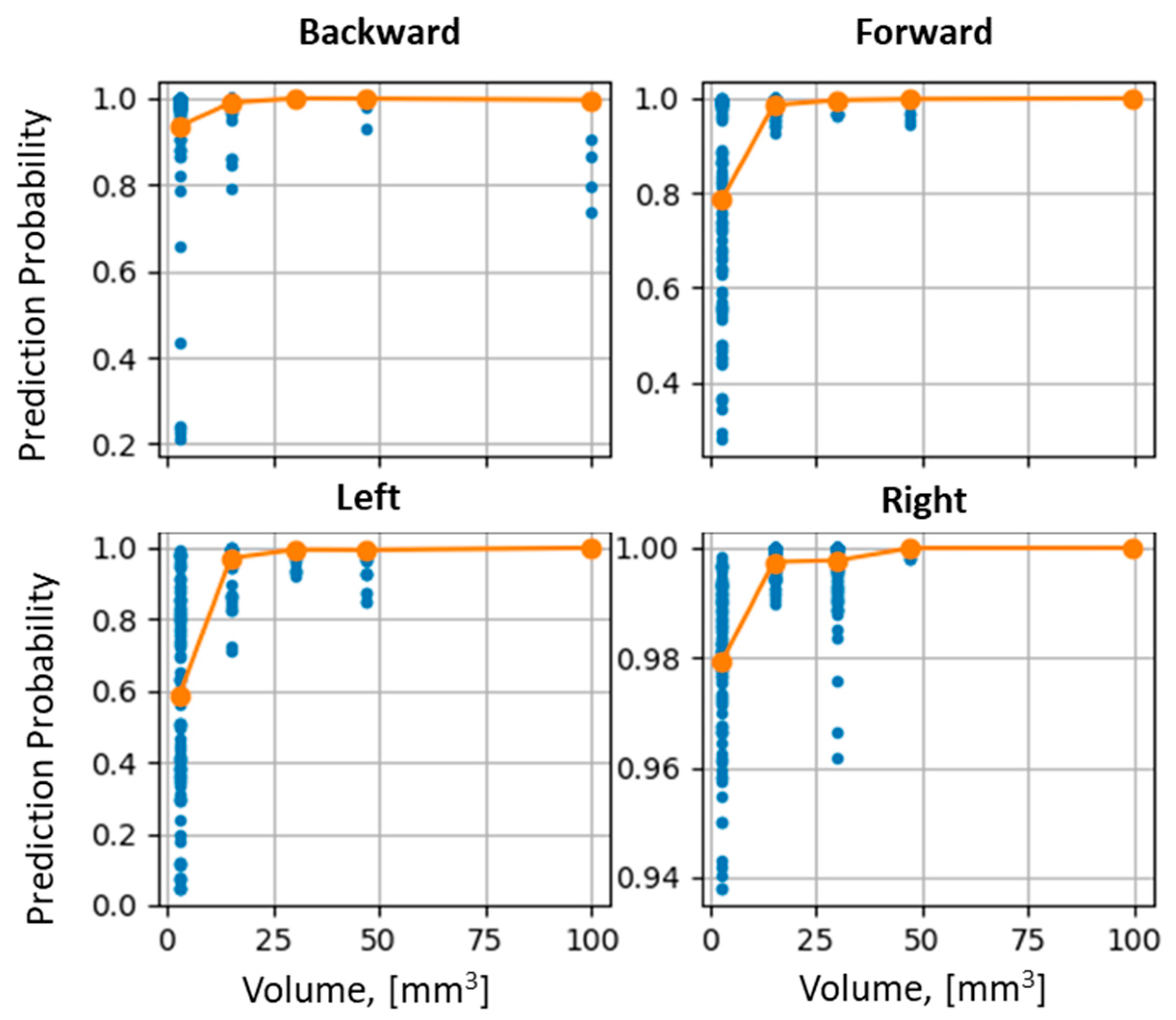
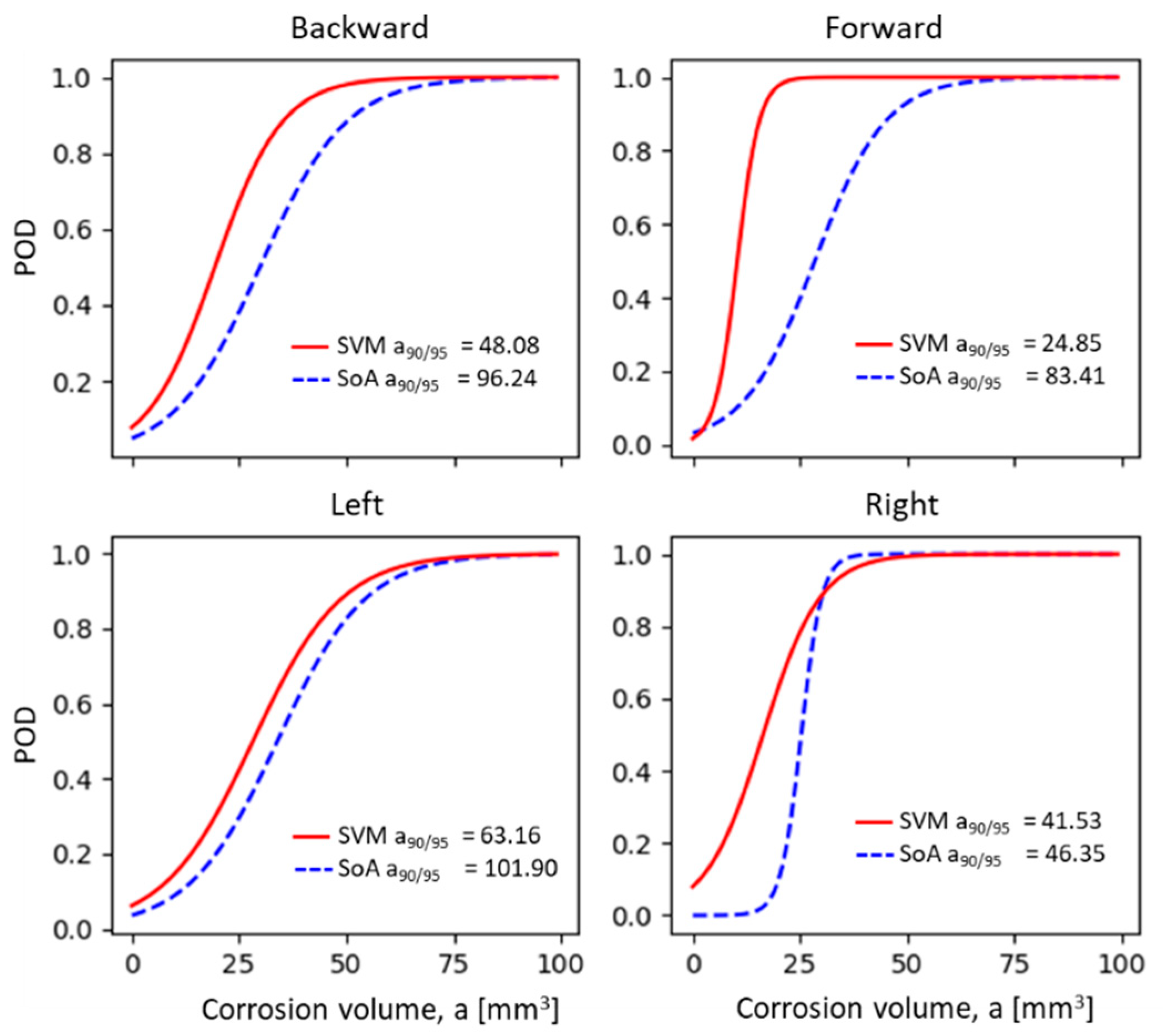
4.4. Probability of Detection
5. Conclusions
Author Contributions
Funding
Conflicts of Interest
References
- Czaban, M. Aircraft Corrosion—Review of Corrosion Processes and its Effects in Selected Cases. Fatigue Aircr. Struct. 2018, 2018, 5–20. [Google Scholar] [CrossRef] [Green Version]
- Hendricks, W.R. The Aloha-airlines accident—A new era for aging aircraft. In Structural Integrity of Aging Airplanes; Atluri, S.N., Sampath, S.G., Tong, P., Eds.; Springer: Berlin/Heidelberg, Germany, 1991; pp. 153–165. [Google Scholar]
- Pitt, S.; Jones, R. Multiple-site and widespread fatigue damage in ageing aircraft. Eng. Fail. Anal. 1997, 4, 237–257. [Google Scholar] [CrossRef]
- Xufei, G.; Yan, H. Ultrasonic Total Focusing Imaging Method of Multilayer Composite Structures Using the Root-Mean-Square (RMS) Velocity. Adv. Mater. Sci. Eng. 2021, 2021, 2745732. [Google Scholar]
- Ruikun, W.; Hong, Z.; Ruizhen, Y.; Wenhui, C.; Guotai, C. Nondestructive Testing for Corrosion Evaluation of Metal under Coating. Adv. Mater. Sci. Eng. 2021, 2021, 6640406. [Google Scholar]
- Kuts, Y.V.; Yeremenko, V.S.; Monchenko, E.V.; Protasov, A.G. Ultrasound method of multilayer material thickness measurement. AIP Conf. Proc. 2009, 1096, 1115–1120. [Google Scholar] [CrossRef]
- Fitzpatrick, G.; Thome, D.; Skaugset, R.; Shih, E.; Shih, W. Magneto-optical/ Eddy current imaging of aging aircraft—A New NDI Technique. Mater. Eval. 1993, 51, 1402–1407. [Google Scholar]
- Thome, D.K.; Fitzpatrick, G.L.; Skaugset, R.L.; Shih, W.C.L. Aircraft corrosion and defect inspection using advanced magneto-optic imaging technology. Proc. SPIE 1996, 2945, 365–373. [Google Scholar]
- Sasi, B.; Rao, B.P.C.; Jayakumar, T.; Raj, B. Development of Eddy Current Test Procedure for Non-destructive Detection of Fatigue Cracks and Corrosion in Rivets of Air-intake Structures. Def. Sci. J. 2009, 59, 106–112. [Google Scholar] [CrossRef] [Green Version]
- Karpenko, O.; Efremov, A.; Ye, C.; Udpa, L. Multi-frequency fusion algorithm for detection of defects under fasteners with EC-GMR probe data. NDT E Int. 2020, 110, 102227. [Google Scholar] [CrossRef]
- Chady, T.; Okarma, K.; Mikołajczyk, R.; Dziendzikowski, M.; Synaszko, P.; Dragan, K. Extended Damage Detection and Identification in Aircraft Structure Based on Multifrequency Eddy Current Method and Mutual Image Similarity Assessment. Materials 2021, 14, 4452. [Google Scholar] [CrossRef]
- Sophian, A.; Gui, Y.T.; Taylor, D.; Rudlin, J. A feature extraction technique based on principal component analysis for pulsed Eddy current NDT. NDT E Int. 2003, 36, 37–41. [Google Scholar] [CrossRef]
- Abidin, I.Z.; Mandache, C.; Tian, G.Y.; Morozov, M. Pulsed eddy current testing with variable duty cycle on rivet joints. NDT E Int. 2009, 42, 599–605. [Google Scholar] [CrossRef]
- Kim, J.; Yang, G.; Udpa, L.; Udpa, S. Classification of pulsed eddy current GMR data on aircraft structures. NDT E Int. 2010, 43, 141–144. [Google Scholar] [CrossRef]
- Horan, P.; Lowerhill, P.R.; Krause, T.W. Pulsed eddy current detection of defects in F/A-18 inner wing spar without wing skin removal using modified principal component analysis. NDT E Int. 2013, 44, 21–27. [Google Scholar] [CrossRef]
- Stott, C.A.; Underhill, P.R.; Babbar, V.K.; Krause, T.W. Pulsed Eddy Current Detection of Cracks in Multilayer Aluminum Lap Joints. Sens. J. IEEE 2015, 15, 956–962. [Google Scholar] [CrossRef]
- Postolacheab, O.; Ribeiroac, A.L.; Ramos, H.G. GMR array uniform eddy current probe for defect detection in conductive specimens. Measurement 2013, 46, 4369–4378. [Google Scholar] [CrossRef]
- Tianyu, D.; Zhaohe, Y.; Hua, H.; Pingjie, H.; Dibo, H.; Guangxin, Z. A method for characterizing defects in multilayer conductive structures by combining pulsed eddy current signals with PCA components. AIP Conf. Proc. 2019, 2102, 80003. [Google Scholar] [CrossRef]
- Fu, X.; Zhang, C.; Peng, X.; Jian, L.; Liu, Z. Towards end-to-end pulsed eddy current classification and regression with CNN. In Proceedings of the IEEE International Instrumentation and Measurement Technology Conference (I2MTC), Auckland, New Zealand, 20–23 May 2019; pp. 1–5. [Google Scholar]
- Huang, P.; Luo, X.; Hou, D.; Yang, Z.; Zhao, L.; Zhang, G. Lift-off nulling and internal state inspection of multilayer conductive structures by combined signal features in pulsed eddy current testing. Nondestruct. Test. Eval. 2018, 33, 272–279. [Google Scholar] [CrossRef]
- Le, M.; Kim, J.; Kim, S.; Wang, D.; Hwang, Y.; Lee, J. Nondestructive Evaluation Algorithm of Fatigue Cracks and Far-side Corrosion around a Rivet Fastener in Multi-layered Structures. J. Mech. Sci. Technol. 2016, 30, 4205–4215. [Google Scholar] [CrossRef]
- Kim, J.; Le, M.; Lee, J.; Kim, S.; Hwang, Y. Nondestructive evaluation of far-side corrosion around a rivet in a multilayer structure. RNDE 2016, 29, 1–20. [Google Scholar] [CrossRef]
- Chollet, N.S.; Solignac, A.; Lecoeur, M.P.; Fermon, C. MR sensors arrays for eddy current testing. In Proceedings of the 11th International Symposium on NDT in Aerospace (AeroNDT 2019), Paris-Saclay, France, 13–15 November 2019. [Google Scholar]
- Aldrin, J.C.; Motes, D.; Forsyth, D.S. Enhanced image processing methods for GMR array inspections of multilayer metallic structures. AIP Conf. Proc. 2013, 1511, 699–706. [Google Scholar] [CrossRef]
- Cristianini, N.; Shawe-Taylor, J. An Introduction to Support Vector Machines and Other Kernel-Based Learning Methods; Cambridge University Press: Cambridge, UK, 2000. [Google Scholar] [CrossRef]
- Annis, C. R Package mh1823, Version 4.0.1. Available online: https://statistical-engineering.com/mh1823/ (accessed on 15 February 2022).


| Components | Properties | |
|---|---|---|
| Sensor probe | Core | Thin slices: 10 Material: Silicon steel Size: 13 × 20 × 50 mm (inner dia., outer dia., height) |
| Coil | Turns: 1220 Copper wire: 0.2 mm diameter Current supply: 0.1 A Frequency: 900 Hz | |
| Hall sensor array | Hall elements: 64 InSb Element interval: 0.52 mm Length: 33.28 mm | |
| Signal processing | High-pass filter | Type: RC Cut-off frequency: 284 Hz To remove low-frequency noise signal |
| Amplifier | Differential type: INA128 No. of elements: 64 Gain: 60 dB | |
| RMS circuits | AD8436 chipset No. of elements: 64 | |
| ADC | Device: NI-PCI 6071E Channels: 64 Resolutions: 12-bit, 2.441 mV/bit Sampling rate: 1.25 MS/s Sampling trigger at each 0.5 mm from XY-stage scanner | |
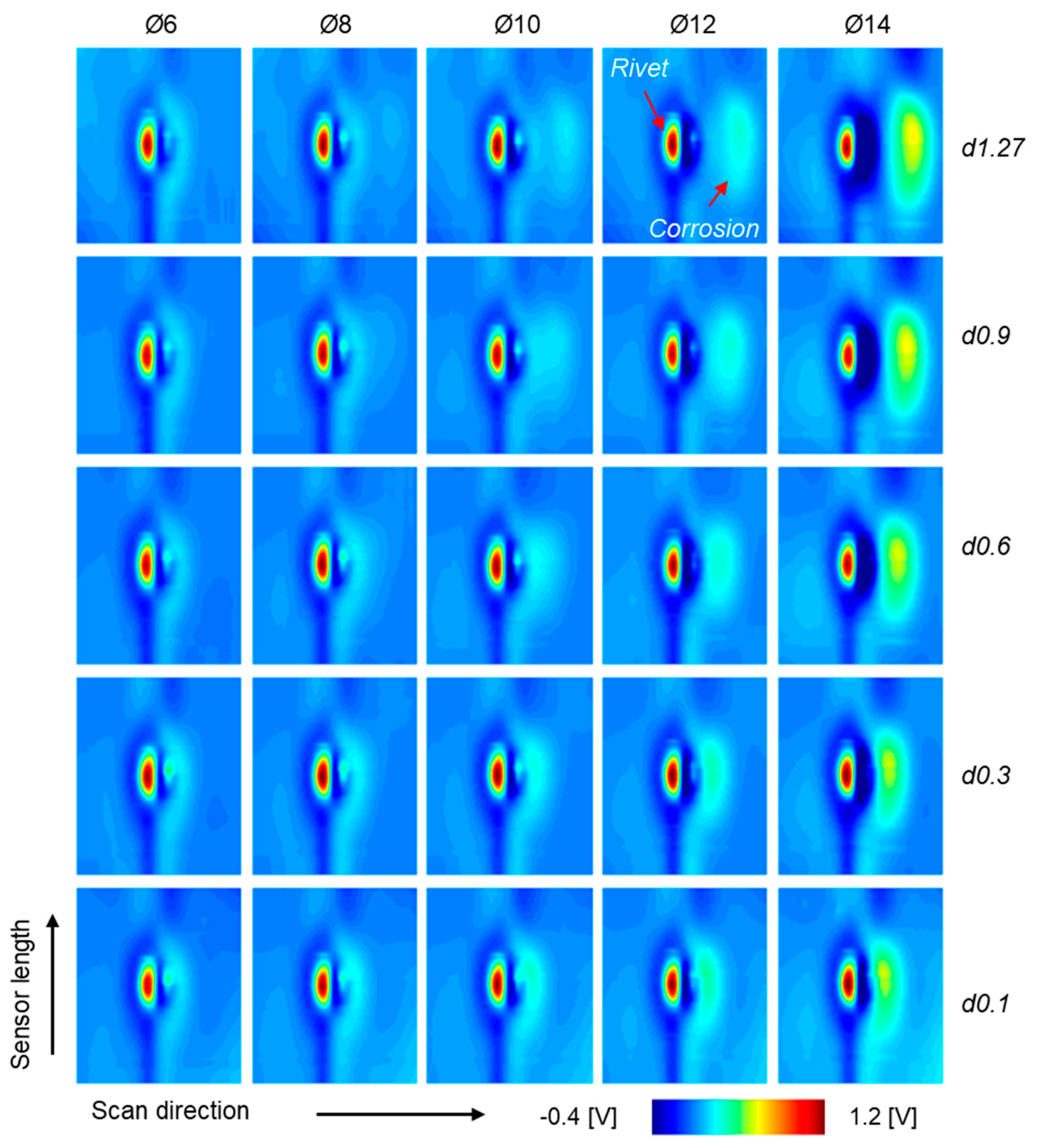
| Specimen & Corrosion | Specimen | Two aluminum alloy layers (Al 2024) Size: 300 × 300 × 1.27 mm No. of Rivets: 25 (AN426 AD-5-6, Air Force and Navy standard) |
| Artificial Corrosion | No. of corrosion: 25 Diameters: 6, 8, 10, 12, 14 mm Depths: 0.1, 0.3, 0.6, 0.9, 1.27 mm (Through) Volumes: 2.8~195.4 mm3 On rivet sites of the second layer |
| Data Splitting Strategy | Training Dataset (The Remained Data Is in the Validation Dataset) | |
|---|---|---|
| Amount of Data | Distinguished Volumes | |
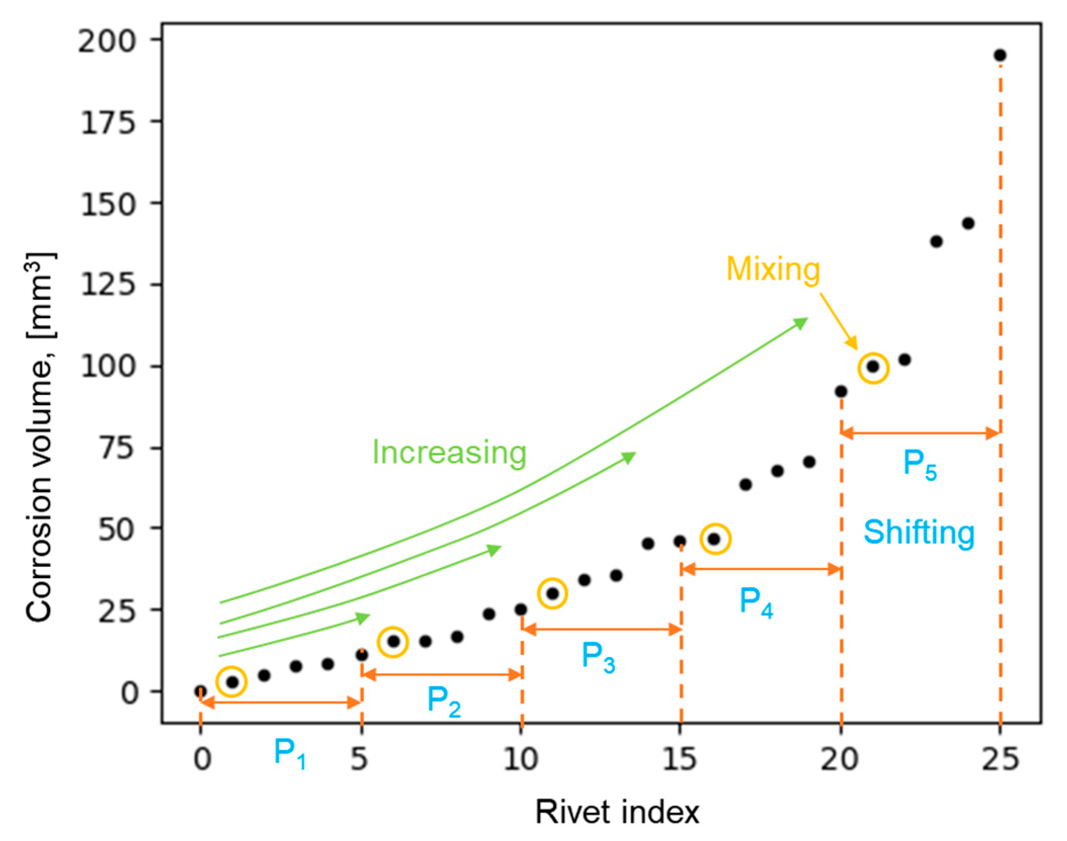
| Mixing | 80% of data | 5 volumes selected from small to large with a step of 5 |
| Increasing | 10%, 20%, 30%, 40%, 50%, 60%, 70%, 80% of data | With respect to 2, 5, 7, 10, 12, 15, 17, 20 volumes increasing from small to large |
| Shifting | Fixed 20% of data for all shifting ranges | Volume in a range: P1, P2, P3, P4, P5 |
| Corrosion | SoA Method [22] | SVM Using 20% Data for Training | ||||
|---|---|---|---|---|---|---|
| Accuracy | F1 Score | AUC | Accuracy | F1 Score | AUC | |
| Backward | 60.0 | 89.58 | 89.58 | 89.58 | 89.90 | 98.45 |
| Forward | 56.0 | 85.42 | 85.42 | 85.42 | 91.53 | 96.52 |
| Right | 64.0 | 91.67 | 91.67 | 91.67 | 93.62 | 98.58 |
| Left | 61.0 | 80.21 | 80.21 | 80.21 | 86.36 | 95.88 |
| Corrosion | SoA Method [22] | SVM Using 20% Data for Training | ||
|---|---|---|---|---|
| a90 | a90/95 | a90 | a90/95 | |
| Backward | 51.91 | 96.24 | 36.55 | 48.08 |
| Forward | 46.65 | 83.41 | 16.02 | 24.85 |
| Right | 30.53 | 46.35 | 31.08 | 41.53 |
| Left | 56.55 | 101.90 | 50.92 | 63.16 |
Publisher’s Note: MDPI stays neutral with regard to jurisdictional claims in published maps and institutional affiliations. |
© 2022 by the authors. Licensee MDPI, Basel, Switzerland. This article is an open access article distributed under the terms and conditions of the Creative Commons Attribution (CC BY) license (https://creativecommons.org/licenses/by/4.0/).
Share and Cite
Le, M.; Luong, V.S.; Nguyen, D.K.; Le, D.-K.; Lee, J. Auto-Detection of Hidden Corrosion in an Aircraft Structure by Electromagnetic Testing: A Machine-Learning Approach. Appl. Sci. 2022, 12, 5175. https://0-doi-org.brum.beds.ac.uk/10.3390/app12105175
Le M, Luong VS, Nguyen DK, Le D-K, Lee J. Auto-Detection of Hidden Corrosion in an Aircraft Structure by Electromagnetic Testing: A Machine-Learning Approach. Applied Sciences. 2022; 12(10):5175. https://0-doi-org.brum.beds.ac.uk/10.3390/app12105175
Chicago/Turabian StyleLe, Minhhuy, Van Su Luong, Dang Khoa Nguyen, Dang-Khanh Le, and Jinyi Lee. 2022. "Auto-Detection of Hidden Corrosion in an Aircraft Structure by Electromagnetic Testing: A Machine-Learning Approach" Applied Sciences 12, no. 10: 5175. https://0-doi-org.brum.beds.ac.uk/10.3390/app12105175