Measurement of Bridge Vibration by UAVs Combined with CNN and KLT Optical-Flow Method

Abstract

A measurement method of bridge vibration by unmanned aerial vehicles (UAVs) combined with convolutional neural networks (CNNs) and Kanade–Lucas–Tomasi (KLT) optical-flow method is proposed. In this method, the stationary reference points in the structural background are required, a UAV is used to shoot the structure video, and the KLT optical-flow method is used to track the target points on the structure and the background reference points in the video to obtain the coordinates of these points on each frame. Then, the characteristic relationship between the reference points and the target points can be learned by a CNN according to the coordinates of the reference points and the target points, so as to correct the displacement time–history curves of target points containing the false displacement caused by the UAV’s egomotion. Finally, operational modal analysis (OMA) is used to extract the natural frequency of the structure from the displacement signal. In addition, the reliability of UAV measurement combined with CNN is proved by comparing the measurement results of the fixed camera and those of UAV combined with CNN, and the reliability of the KLT optical-flow method is proved by comparing the tracking results of the digital image correlation (DIC) and KLT optical-flow method in the experiment of this paper.

1. Introduction

The long-term use of bridges may lead to structural damages; hence, it is necessary to detect damages regularly. Vibration measurement is an important step in structural damage detections. In recent years, some noncontact-measurement methods have been proposed, such as Global Positioning System (GPS) [1] and laser Doppler vibrometer (LDV) [2], to replace the traditional contact-measurement methods (such as acceleration sensors [3] and strain gauges [4]). However, the GPS is of low accuracy [5] and LDV is costly and time-consuming [6]. With the development of computer-vision technology, digital image correlation (DIC) is more and more widely used in bridge vibration measurement [7,8]. Compared with GPS and LDV, DIC technology has the advantages of low cost, high precision, and high efficiency. DIC is also used for deformation and displacement measurement of other engineering structures [9]. However, the measurement accuracy of the DIC method is limited due to the errors caused by pixel interpolation [10]. Also as a computer-vision method, the optical-flow method is widely used in bridge vibration measurement, and its accuracy has been confirmed [11,12].

The Kanade–Lucas–Tomasi (KLT) optical-flow method [13] is proposed on the basis of the Lucas–Kanade optical-flow method [14]. The concept of optical flow was first proposed by Gibson [15], and represents the velocity of a moving object in a time-varying image. According to the idea of optical flow, the KLT optical-flow method matches and tracks the feature points of two adjacent frames to obtain the motion information of the feature points. The KLT optical-flow method is widely used in tracking the feature points of different scenes (buildings, grasslands, etc.) to validate its reliability [16] in measuring vibration of bridge models [12].

In order to adapt to various measurement environments (such as cross-river bridges, etc.), in recent years, UAVs have been used to replace fixed cameras for bridge measurement [17,18]. UAVs are also gradually applied to structural crack detection, displacement measurement, and damage inspection of bridges [19,20,21]. However, due to egomotion of UAVs during their flights, the measured displacement includes not only the displacement of the measured structure, but also the false displacement caused by UAV egomotion. The common method to eliminate the false displacement is homography transformation [22,23], but this requires that four or more static reference points are in the same plane of the target points, which is difficult to achieve in actual measurement. The random components in the signals collected by UAVs may be suppressed by a differential filtering method [24] to obtain the structural modal parameters [25]. Although the bridge modal parameters can be extracted by this method without using any reference point, it does not obtain the real displacement time–history curves of the target points. The correction method of three-dimensional reconstruction is proposed to obtain the intrinsic and extrinsic parameters of the UAV cameras by using Zhang’s method [26], so as to recover the 3D world coordinates of the structure to obtain its true displacement [27]. However, this method requires that the plane of the reference points is parallel to that of the target points and the distance between the two planes is known, which is difficult to achieve in practical measurement. The correction of UAV images by neural networks has attracted much attention in recent years. The method of correcting UAV images with a radial basis function (RBF) neural network is proposed [28]. The selected control points are used by this method as the training samples of the network. The corrected images can be obtained after the UAV images are inputted into the network. The two-layer feedforward neural network (FNN) was used to learn the characteristic relationship between the reference background and target points from the video with no structural motion [29]. The target-point coordinates can be estimated through the reference background when the structure is vibrating, which can be used to determine the homography transformation matrix of each frame image, so as to obtain the real coordinates of the target points.

A measurement method of bridge vibration by UAVs based on the KLT optical-flow method and a CNN is proposed in this paper. In this method, the KLT optical-flow method is used to accurately track the target points, and the multilayer CNN is used to effectively learn the characteristic relationship between the reference points and the target points to eliminate the false displacement of the UAV, so as to obtain the real displacement time–history curves of the structure, and the natural frequency of the model is extracted by OMA [30,31]. Finally, the measurement results of DIC and fixed camera are used as references to validate the reliability of the method proposed by this paper.

2. Methods

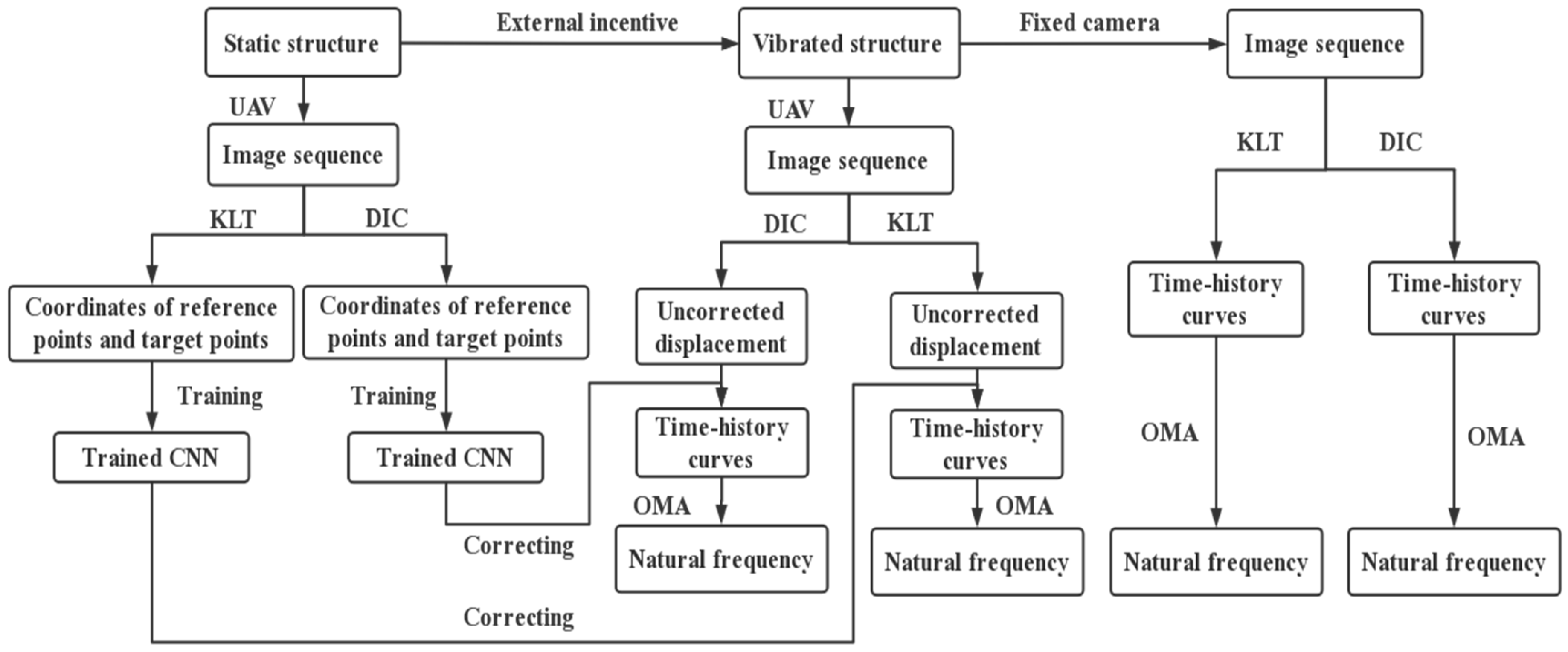
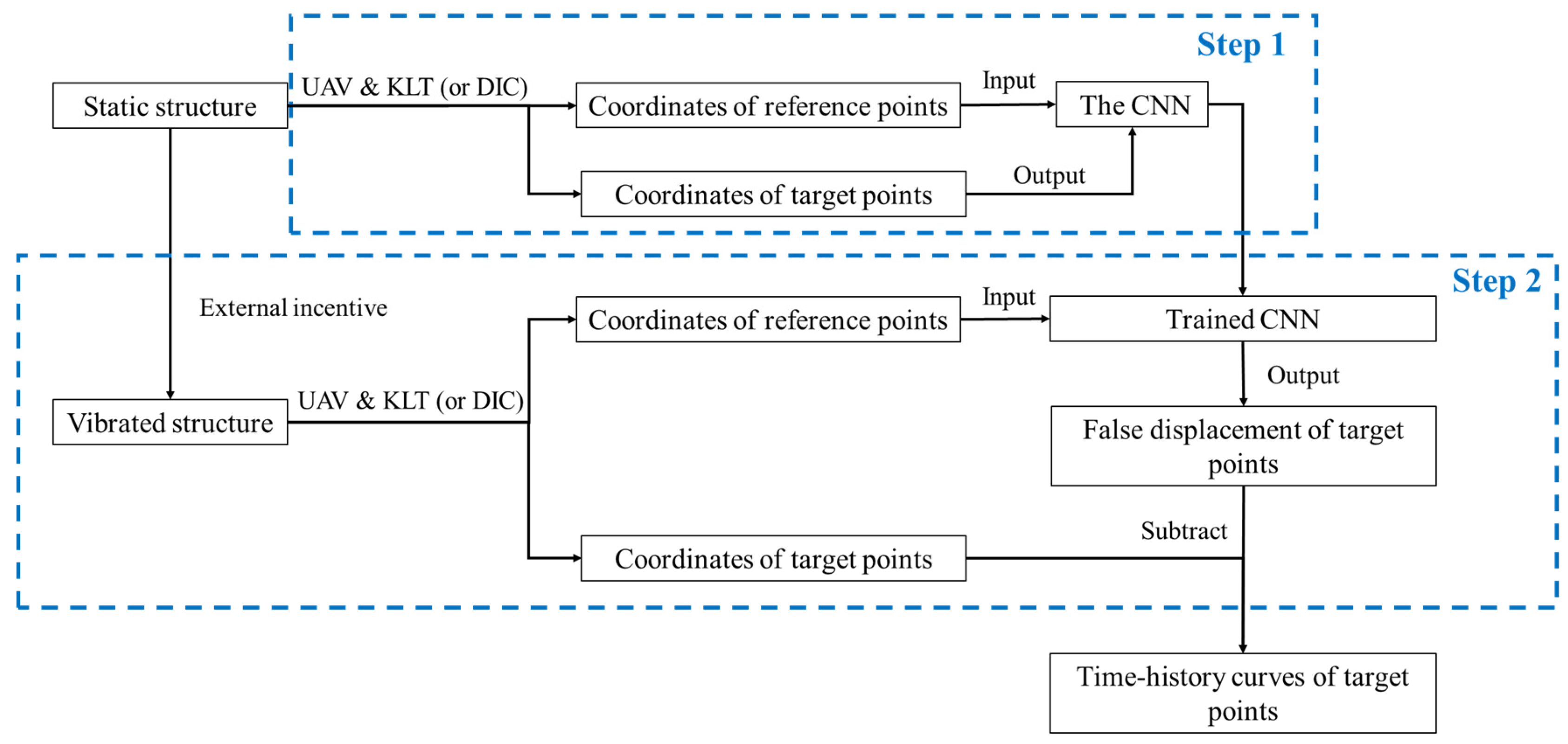
Firstly, the video of a static structure taken by a UAV is converted into a set of continuous digital image sequences stored in the frame form. The coordinates of reference points and target points are obtained by DIC and KLT optical-flow method to train the CNN. Then, the structure is excited and the image sequences are captured by a fixed camera and UAV. The target points are tracked with DIC technology and KLT optical-flow method, respectively, to obtain the displacement time–history curves (the one obtained by the UAV needs to be corrected by a CNN). The natural frequency of the structure is then extracted by OMA. The technical flowchart is shown in Figure 1.

2.1. KLT Optical-Flow Method

2.1.1. Assumptions of Optical-Flow Method

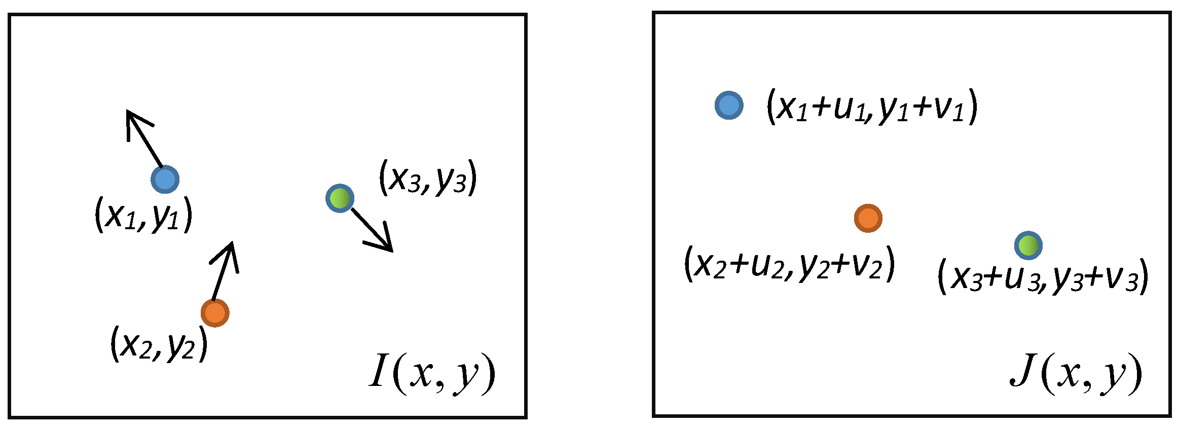
The optical-flow method is based on two assumptions: brightness constancy and small motion; that is, the pixel value of the same points between frames are unchanged and the motion of the points is small. Figure 2 shows three target points in two adjacent images. The position of the target points in the second image can be determined by finding the point whose pixel value is consistent with the target points in the first image.

2.1.2. KLT Optical-Flow Method

In addition to the two assumptions, the KLT optical-flow method [13] also assumes the spatial consistency; that is, the adjacent pixels in the previous frame are also adjacent in the next frame.

Suppose $I_1\left(x,y\right)$ and $I_2\left(x,y\right)$ are two adjacent images; a fixed size window, $W$, centered on the position of a target point is established in the first image. All pixels in $W$ move $\left(d_x,d_y\right)$ between the two images, and $\left(x,y\right)$ are the coordinates of pixels. Let $\mathit{d}={\left[\begin{array}{cc}{d}_x& d_x\end{array}\right]}^T$, $\mathit{X}={\left[\begin{array}{cc}x& y\end{array}\right]}^T$. The $\mathit{d}$ closest to the actual value can be obtained by minimizing the following expression:

$$\epsilon ={{\displaystyle \iint }}_W^{ }{\left[I_2\left(\mathit{X}\right)-I_1\left(\mathit{X}-\mathit{d}\right)\right]}^2\omega \left(\mathit{X}\right)d\mathit{X}.$$

(1)

where $\omega \left(\mathit{X}\right)$ is a weighting function. In the simplest case, $\omega \left(\mathit{X}\right)=1$. Alternatively, $\omega$ could be a Gaussian-like function to emphasize the central area of the window. Move the centers of $I_1$ and $I_2$ by $\mathit{d}/2$ to obtain

$$\epsilon ={{\displaystyle \iint }}_W^{ }{\left[I_2\left(\mathit{X}+\frac{\mathit{d}}{2}\right)-I_1\left(\mathit{X}-\frac{\mathit{d}}{2}\right)\right]}^2\omega \left(\mathit{X}\right)d\mathit{X}.$$

(2)

Set the partial derivative of $\epsilon$ with respect to $\mathit{d}$ as 0:

$$2{{\displaystyle \iint }}_W^{ }\left[I_2\left(\mathit{X}+\frac{\mathit{d}}{2}\right)-I_1\left(\mathit{X}-\frac{\mathit{d}}{2}\right)\right]\left[\frac{\partial I_2\left(\mathit{X}+\frac{\mathit{d}}{2}\right)}{\partial \mathit{d}}-\frac{\partial I_1\left(\mathit{X}-\frac{\mathit{d}}{2}\right)}{\partial \mathit{d}}\right]\omega \left(\mathit{X}\right)d\mathit{X}=0.$$

(3)

The following formula can be obtained from Taylor’s expansion:

$$I_2\left(\mathit{X}+\frac{\mathit{d}}{2}\right)\approx I_2\left(\mathit{X}\right)+\frac{d_x}{2}\frac{\partial I_2}{\partial x}\left(\mathit{X}\right)+\frac{d_y}{2}\frac{\partial I_2}{\partial y}\left(\mathit{X}\right).$$

(4)

$$I_1\left(\mathit{X}-\frac{\mathit{d}}{2}\right)\approx I_1\left(\mathit{X}\right)-\frac{d_x}{2}\frac{\partial I_1}{\partial x}\left(\mathit{X}\right)-\frac{d_y}{2}\frac{\partial I_1}{\partial y}\left(\mathit{X}\right).$$

(5)

Substitution of Equations (4) and (5) into Equation (3) leads to

$${{\displaystyle \iint }}_W^{ }\left[I_2\left(\mathit{X}\right)-I_1\left(\mathit{X}\right)+{\mathit{p}}^T\mathit{d}\right]\mathit{p}\left(\mathit{X}\right)\omega \left(\mathit{X}\right)d\mathit{X}=0.$$

(6)

where

$$\mathit{p}={\left[\begin{array}{cc}\frac{\partial }{\partial x}\left(\frac{I_1+I_2}{2}\right)& \frac{\partial }{\partial y}\end{array}\left(\frac{I_1+I_2}{2}\right)\right]}^T.$$

(7)

The following equation can be obtained from Equation (6):

$$Z\mathit{d}=e.$$

(8)

where $Z={{\displaystyle \iint }}_W^{}\mathit{p}\left(\mathit{X}\right){\mathit{p}}^T\left(\mathit{X}\right)\omega \left(\mathit{X}\right)d\mathit{X}$, $e={{\displaystyle \iint }}_W^{}\left[I_1\left(\mathit{X}\right)-I_2\left(\mathit{X}\right)\right]\mathit{p}\left(\mathit{X}\right)\omega \left(\mathit{X}\right)d\mathit{X}$.

Equation (8) can be solved by an iterative method to obtain the value of $\mathit{d}$. When the value of $e$ is less than the set threshold, the approximate solution of $\mathit{d}$ can be obtained.

In this paper, the process of tracking the target point on the bridge model by the KLT optical-flow method is as follows:

• Select the target point in the initial image;
• Based on the local template of each target point, the vector of the point between adjacent frames can be found [13];
• The tracking effect is judged in each image to optimize the result for each target point.

2.1.3. KLT Optical-Flow Method under Pyramid

It can be seen from Section 2.1.2 that if the assumption of small motion is not met, the Taylor expansion of Equations (4) and (5) cannot be carried out. The image pyramid [32] referred by the KLT optical-flow method is used in this paper, which can effectively solve the above problem. Suppose there is an 800 × 800 image, the displacement range of the target point in this image is 32 × 32. Now the image is reduced to 400 × 400, the displacement range of the target point is reduced to 16 × 16, and the assumption of small motion can be met again according to this principle.

The specific principle of KLT optical-flow method under the pyramid is as follows. For each image, the original image is taken as layer 0, and the image reduced by 2^L times in length and width is taken as layer L. The obtained image is superimposed from bottom to top to generate the Gaussian pyramid shown in Figure 3. The displacement value of the target point on the highest layer is calculated in the way of the previous section, which is taken as the initial value of the optical-flow calculation of the next layer to calculate the accurate displacement value of this layer. The calculated displacement value is transmitted to the next layer again, so as to calculate to the lowest layer (level 0) to obtain the real displacement value.

2.2. DIC Technology

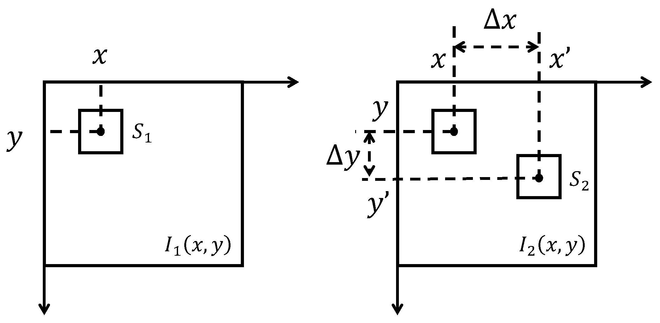
The principle of DIC method is shown in Figure 4: $I_2\left(x,y\right)$ is the deformed image of the image $I_1\left(x,y\right)$; $S_1$ centered on $\left(x,y\right)$ and $S_2$ centered on $\left(x^{\prime },y^{\prime }\right)$ are two windows with the same size, $S$, which are established at $I_1\left(x,y\right)$ and $I_2\left(x,y\right)$, respectively. Where $x^{\prime }=x+∆x$, $y^{\prime }=y+∆y$. The correlation between two windows can be expressed as [33]:

$$C\left(∆x,∆y\right)=\frac{{{\displaystyle \iint }}_S^{ }{I}_1\left(x,y\right)I_2\left(x+∆x,y+∆y\right)dxdy}{\sqrt{{{\displaystyle \iint }}_S^{ }{I}_1^2\left(x,y\right)dxdy}·\sqrt{{{\displaystyle \iint }}_S^{ }{I}_2^2\left(x+∆x,y+∆y\right)dxdy}}.$$

(9)

The real displacement of $\left(x,y\right)$ between two images, $\left(∆x,∆y\right)$, can be obtained when the function value of $C\left(∆x,∆y\right)$ is the maximum.

A fixed-size window is used by both DIC and KLT optical-flow methods to search target points in the whole image range; however, the two methods are different in tracking target points. As shown in Equation (1), the target tracking of KLT optical-flow method is based on the residual error of a fixed-size window between two frames, while that of DIC is based on the correlation of a fixed-size window between two frames, as shown in Equation (9). Moreover, the implementation process of KLT optical-flow method is accompanied by the image-pyramid technology, which tracks the points at multiple levels of resolution of an image to optimize tracking effect to improve the tracking accuracy.

2.3. Convolutional Neural Networks

The false displacement caused by UAV measurement can be removed by a CNN. As a feedforward neural network, each neuron of the CNN only extracts the local information of the input data, and the information are collected at a higher level of the network to obtain the global information [34]. The complexity of the model is reduced by weight sharing [35], which accelerates the computing speed and improves the calculation accuracy. The following is an introduction to the function layer involved in this paper.

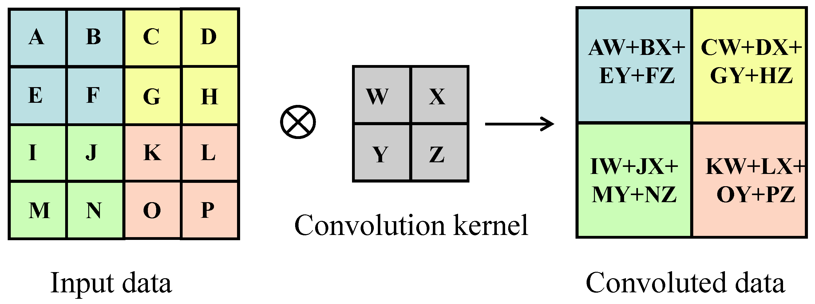
The convolution layer is the core of the whole CNN, and the convolution process is shown in Figure 5. Suppose that there is a 2 × 2 convolution kernel, the sub area consistent with the size of convolution kernel is found in the input data. An element of the new matrix can be obtained by multiplying and summing each corresponding element in the sub area and convolution kernel, and a new matrix can be generated by navigating all of the input data in steps according to the above method.

The feature-extraction ability of the network and the approximation ability of complex functions can be enhanced by activation-function layer. The activation function used in this paper is Leaky Relu, and its expression is as follows:

$$f\left(x\right)=\{\begin{array}{l}x, x\ge 0\\ scale\times x, x<0\end{array}.$$

(10)

The regression layer generally deals with regression problems, and its loss function is expressed as follows:

$$J=\frac{1}{2}{\displaystyle \sum }_{i=1}^R\frac{{\left(t_i-y_i\right)}^2}{R}.$$

(11)

where $R$ is the number of samples, $t_i$ is the target output, and $y_i$ is the prediction output. The value of $J$ will decrease with the training of the network until it converges to the target value.

The network used in this paper is a deep-convolution neural network including input layer, convolution layer, activation-function layer, full-connection layer, normalization layer, and output layer. The architecture of the CNN is shown in Figure 6.

2.4. Operational Modal Analysis

In a multiple-degree-of-freedom system, the expression of the response transmissibility $T_{io}\left(\omega \right)$ [36] is

$$T_{io}\left(\omega \right)=\frac{X_i\left(\omega \right)}{X_o\left(\omega \right)}.$$

(12)

where $X_i\left(\omega \right)$ and $X_o\left(\omega \right)$ are the Fourier transformations of $x_i\left(t\right)$ and $x_o\left(t\right)$ that are the time–history response signals at degrees of freedom $i$ and $o$. The expression of the power spectral density (PSD) transmissibility [37] is

$$\widehat{T_{io}}\begin{array}{c}\left(\omega \right)=\frac{S_{i,o}\left(\omega \right)}{S_{o,o}\left(\omega \right)}\end{array}=\frac{X_i\left(\omega \right)X_o^{*}\left(\omega \right)}{X_o\left(\omega \right)X_o^{*}\left(\omega \right)}=T_{io}\left(\omega \right).$$

(13)

where $S_{o,o}\left(\omega \right)$ is the self-power spectral density of $x_o\left(t\right)$, $S_{i,o}\left(\omega \right)$ is the cross-power spectral density of $x_i\left(t\right)$ and $x_o\left(t\right)$, and $X_o^{*}\left(\omega \right)$ is the conjugate complex number of $X_o\left(\omega \right)$. In this paper, the displacement time–history curves are obtained by KLT optical-flow method and DIC, which are used to obtain the PSD curves. The natural frequencies of the structure are obtained from the peaks of the self PSD curve, while the modal shape can be obtained from the ratios of the PSD transmissibility at corresponding degrees of freedom.

3. Experiment

3.1. Experimental Equipment

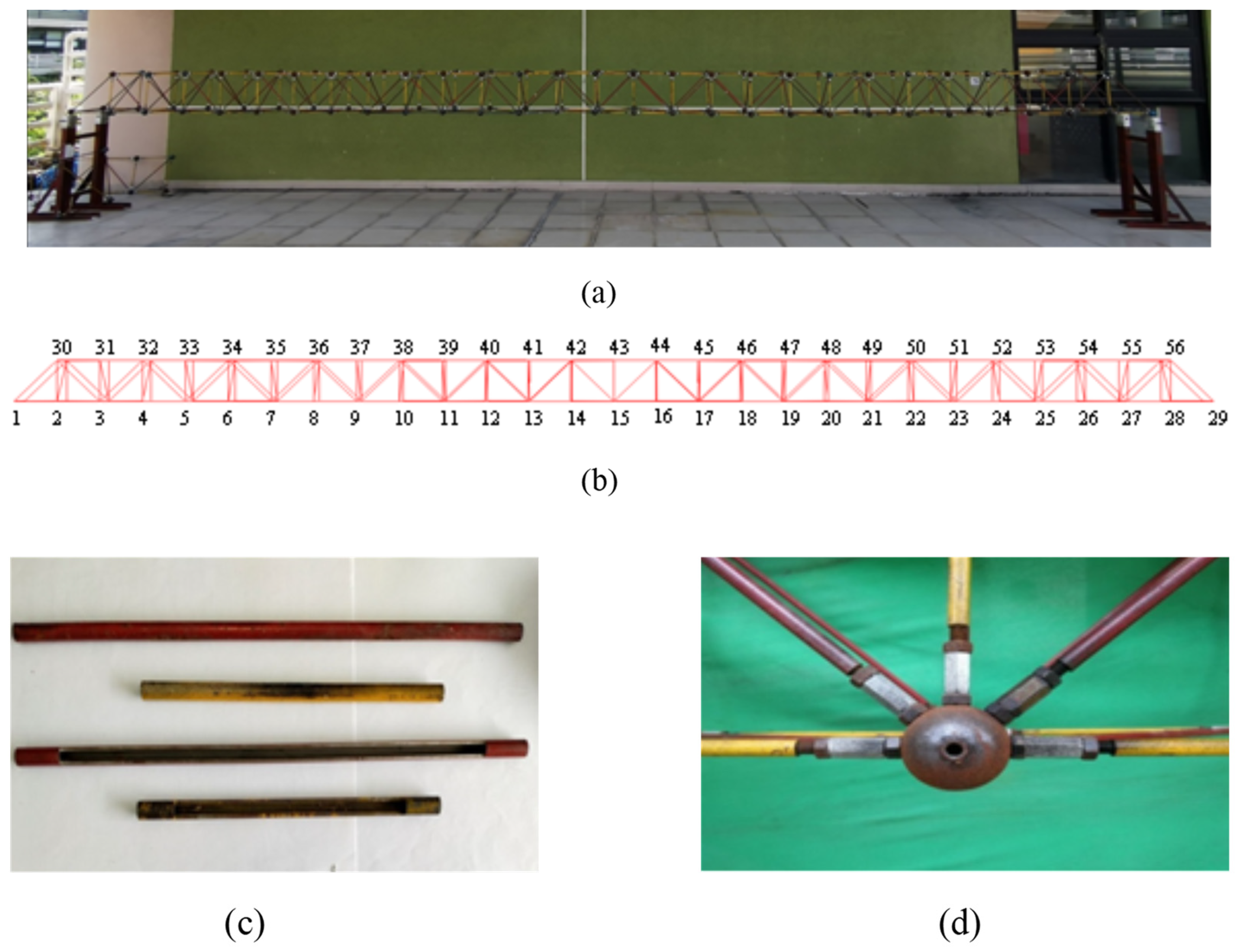
The bridge model used in the experiment is a spatial steel-frame structure with a total length of 9.8 m and 29 nodes (Figure 7a,b). Figure 7c,d show the hollow round bar (Q235 steel), bolts, and connecting balls constituting the model, respectively, in which the lengths of red and yellow hollow round members are 365 mm and 215 mm, respectively. The width and height of each span of the model are 0.35 m.

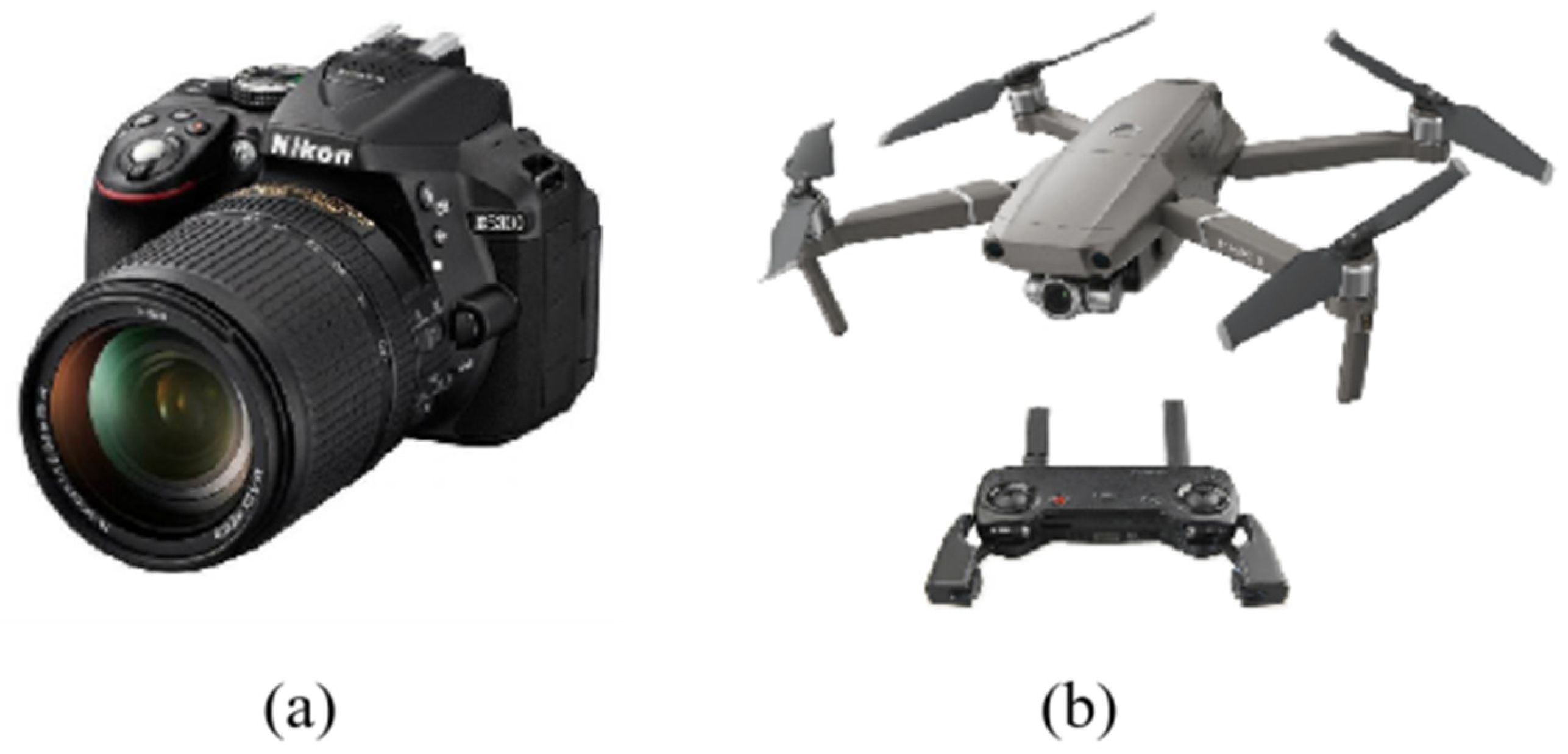
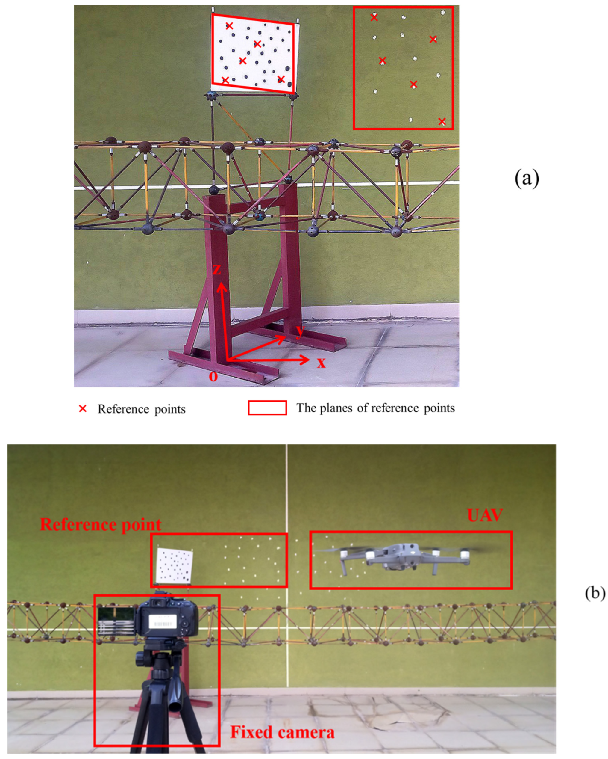
The images of the vibrational model are collected by the fixed camera (D5300, Nikon Corporation, Japan) in Figure 8a and the quad-rotor UAV (Mavic Air 2, Da-Jiang Innovations, Shenzhen, China) in Figure 8b, which are placed 2 m away from the model [8]. The acquisition frequency of the UAV is 30 frames/s and the image resolution is 3840 × 2160. In order to correct the measurement of the UAV, 5 reference points are selected on the cardboard at 45° to the plane of the model; the other 5 reference points are selected on the back wall. Hence, all reference points are not in the same plane. The experimental layout is shown in Figure 9b.

3.2. Experimental Scheme

To validate the reliability of vibration measurement of the bridge model by UAV combined with CNN and KLT optical-flow method, the measurement results of the fixed camera are taken as a reference. Moreover, the measurement results of DIC are taken as a reference to validate whether KLT optical-flow method is feasible to replace DIC in bridge vibration measurement.

Firstly, the fixed camera and UAV are placed about 2 m away from the bridge model, and the UAV is used to shoot the static model (the shooting time is 8 min). The reference-point coordinates tracked by DIC and KLT optical-flow method are used as the input of CNN, and the target-point coordinates are used as the network output to train the network. Secondly, the bridge model is excited to vibrate, the fixed camera and UAV are used to shoot (the shooting time is 80 s for 5 times of excitation), and the points are tracked by DIC and KLT optical-flow method again. The reference-point coordinates measured by the UAV are still taken as the input of CNN, the false displacement of the target points caused by the UAV will be outputted by the trained CNN according to the characteristic relationship between the reference points and the target points, and the real displacements of the target points measured by the UAV are obtained by subtracting the output value from the uncorrected displacement of the target point. The natural frequency of the model is obtained by OMA from the time–history curves. The specific process is shown in Figure 1, and the process of correcting displacement measured by a UAV through the CNN is shown in Figure 10. Finally, the tracking effects of DIC and KLT optical-flow method are compared under the fixed-camera and UAV measurements to validate the feasibility of KLT optical-flow method replacing DIC, and the results of fixed camera and UAV are compared under the KLT optical-flow method to validate the reliability of UAV data combined with CNN and KLT optical-flow method. The DIC, KLT optical-flow method, and CNN are realized using MATLAB (MathWorks Inc., Natick, MA, USA) software.

4. Experimental Results and Analysis

The bridge model used in this paper has the largest displacement at node 15 in the middle of the span. Therefore, in order to better display the results, node 15 is selected as the target point in this paper (See Appendix A for the measurement results of node 5 and node 10).

4.1. Comparisons for DIC and KLT Method

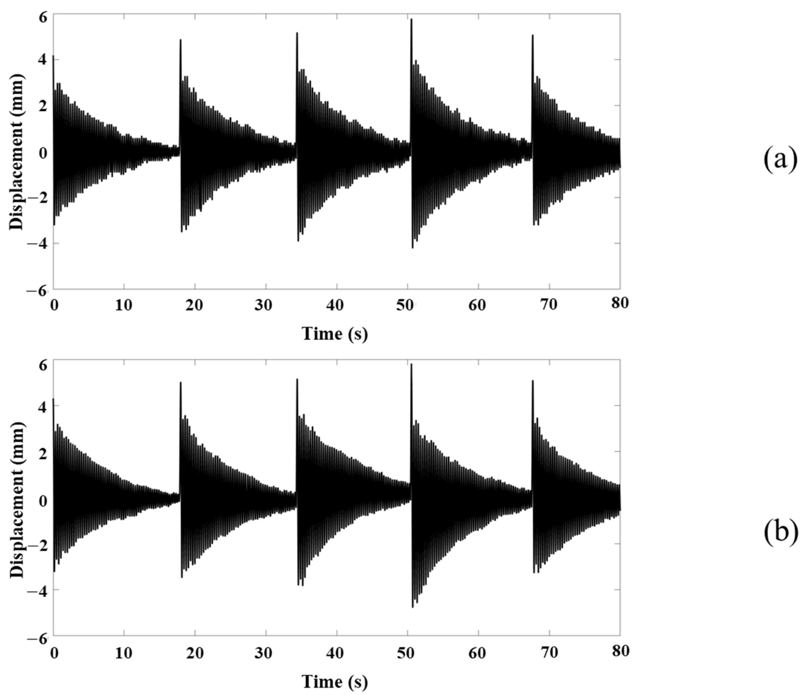
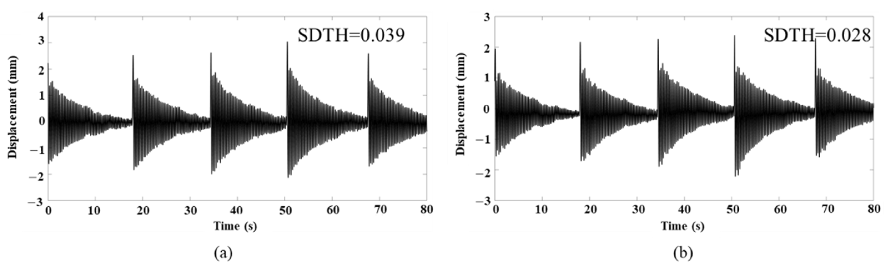
The displacement results of the bridge model measured by fixed camera are showed in Figure 11, which demonstrates that the displacement time–history curves obtained by the DIC and KLT optical-flow method have very similar characteristics of free-vibration attenuation, and the maximum amplitude is about 5.7 mm. The ideal displacement curve $x^{\prime }\left(t\right)$ can be obtained by smoothing the displacement time–history curve $x\left(t\right)$ through locally weighted regression (LOWESS [38]). The difference between $x\left(t\right)$ and $x^{\prime }\left(t\right)$ is the error curve, and the average of the error curve reflects the smoothness of the displacement time–history curve measured by the DIC or KLT optical-flow method, which is defined as SDTH in this paper. The SDTHs of the DIC and KLT optical-flow method are 0.048 and 0.031, respectively. In addition, the displacement time–history curve obtained by DIC has obvious burrs, which illustrates its low measurement accuracy. In contrast, the displacement diagram obtained by the KLT optical-flow method is smoother, indicating that DIC is not as accurate as the KLT optical-flow method.

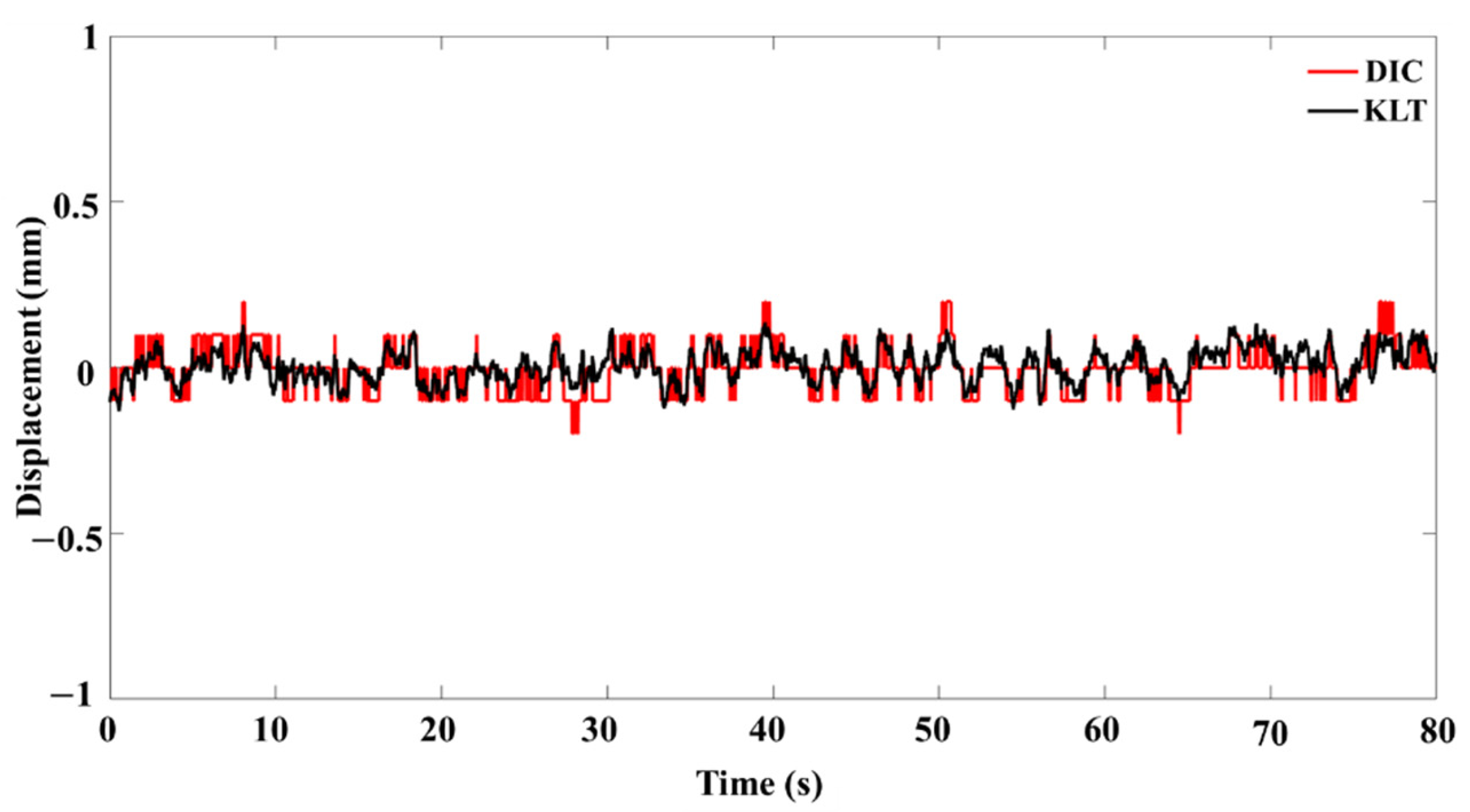
As shown in Figure 12, it is the displacements of the static point on the model measured by the fixed camera and obtained by the DIC and KLT optical-flow method. Theoretically, the curve should be a straight line with displacement of 0, so that the standard deviation (STD) of the curve can reflect the accuracy of the two methods. The STDs of the DIC and KLT optical-flow method are 0.075 and 0.061, respectively, which indicate that the KLT optical-flow method is more accurate than DIC.

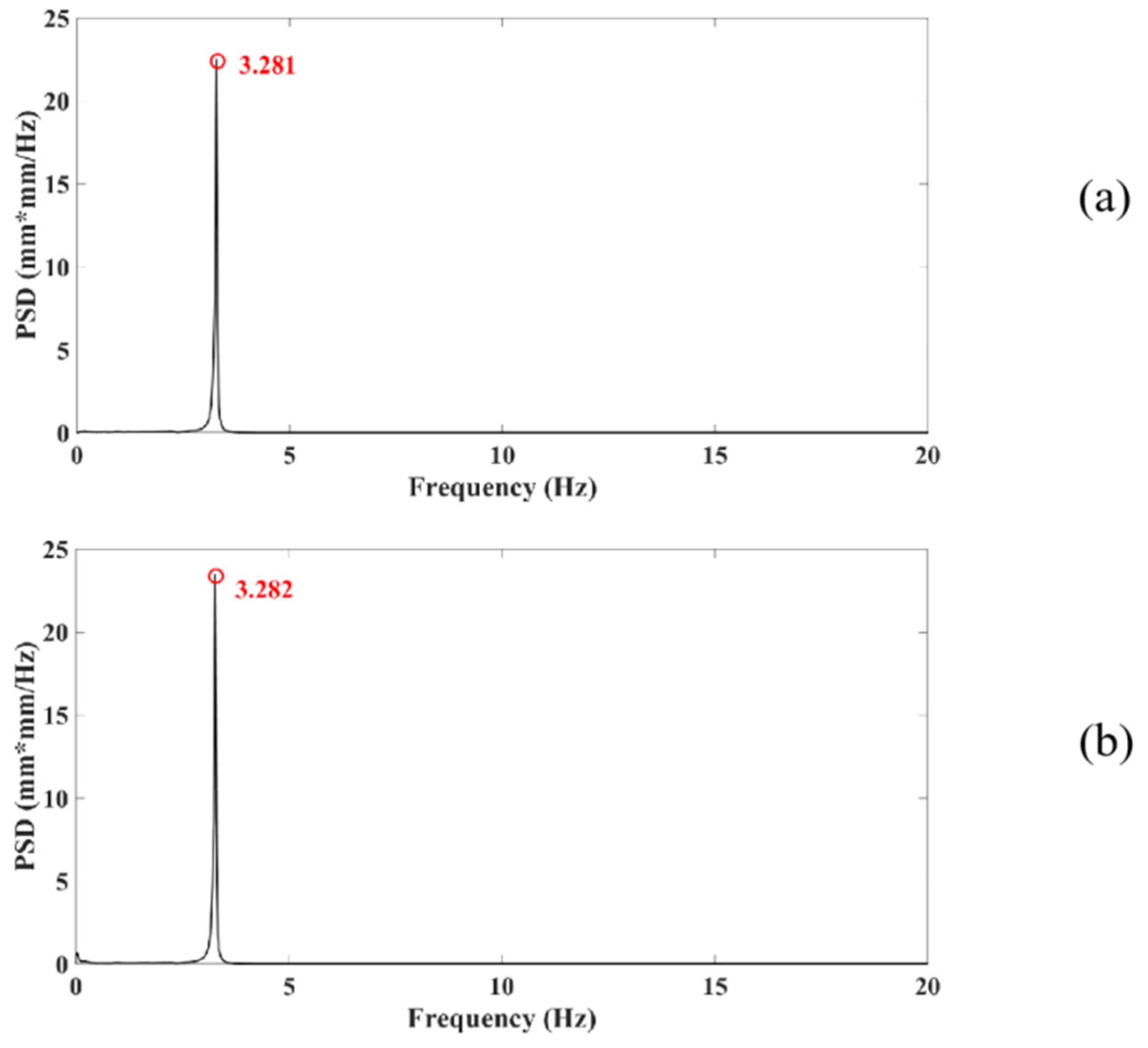
The displacement signals in Figure 11 are processed into PSD curves. The peak of the PSD curve corresponds to the natural first frequency of the model, as shown in Figure 13. It can be seen from the figure that the natural frequencies extracted by the two methods are 3.281 Hz and 3.282 Hz, respectively, and the relative error is 0.03%. It shows that the KLT optical-flow method is feasible to replace DIC to extract the natural frequency of the structure under fixed camera.

4.2. Comparisons of UAV Measurement

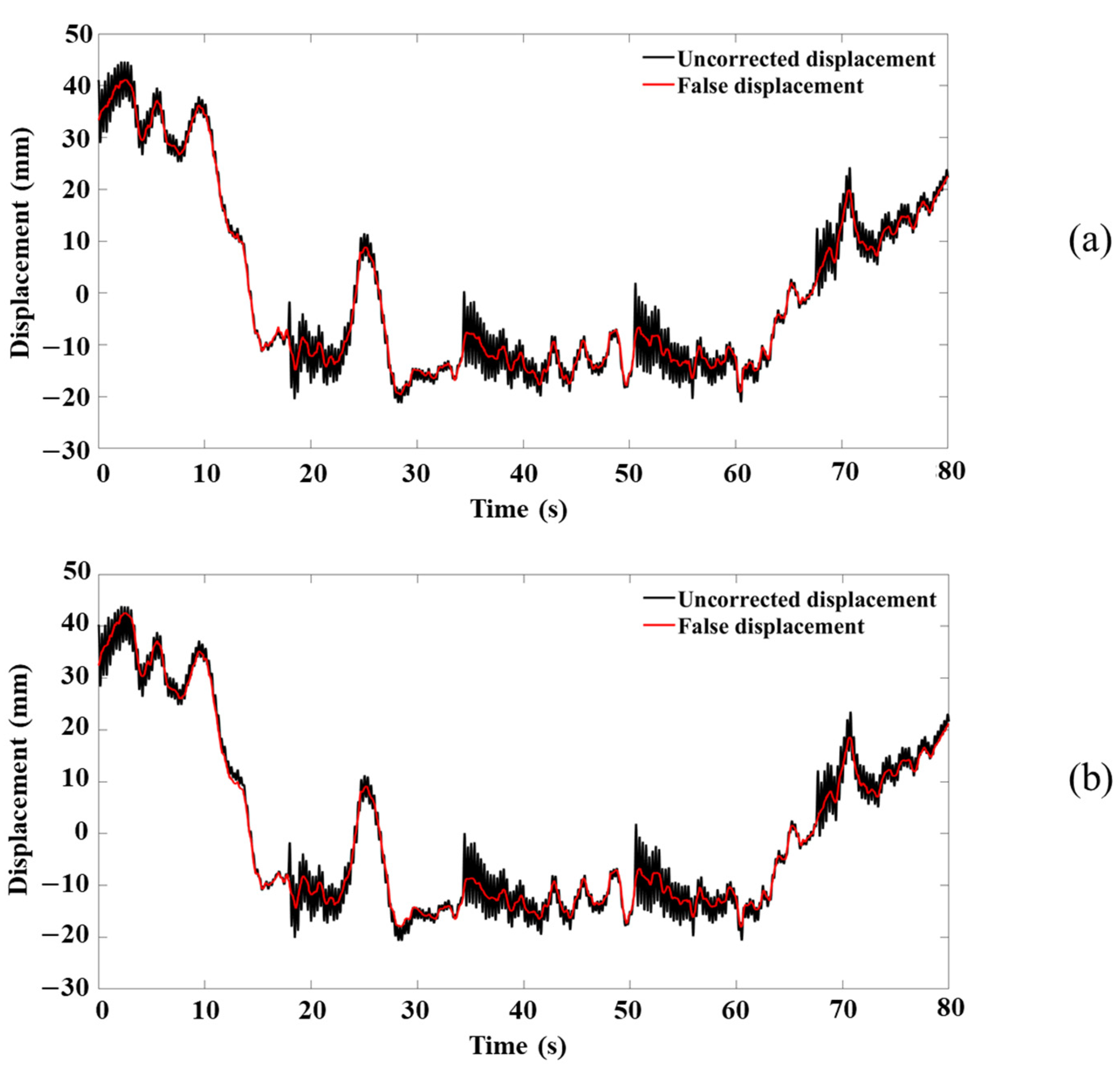
The uncorrected displacement measured by the UAV and the false displacement predicted by the CNN are shown in Figure 14. The figure shows that the uncorrected displacement curves measured by the UAV have serious drift.

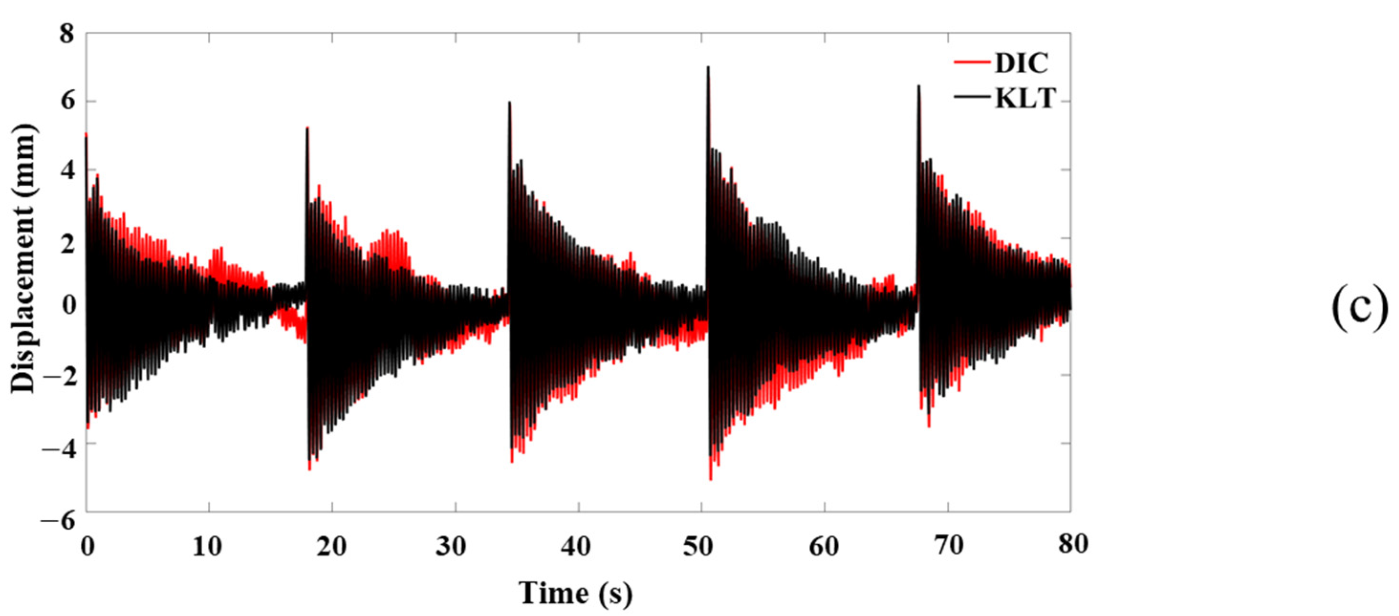
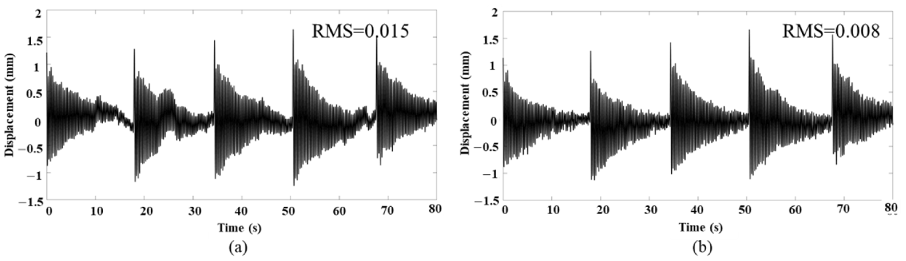
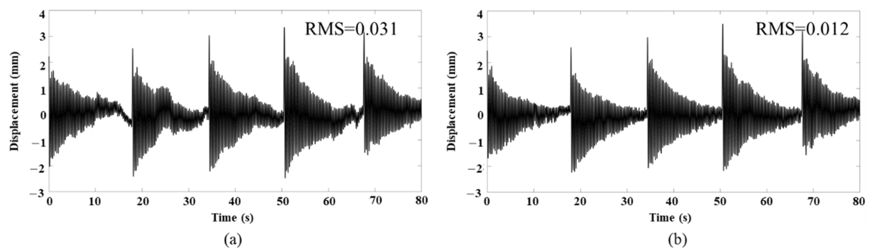
The true displacements of the structure are shown in Figure 15, which are obtained by subtracting the false displacement of the target points predicted by the CNN from the uncorrected displacement of the target points. The corrected displacement curve obtained by DIC has more drift than that by the KLT optical-flow method. In addition, it can be seen from Figure 15 that each wave of displacement time–history curves fluctuates at $Displacement=0$. The greater the drift of the curve, the farther the mean line of each wave is from $Displacement=0$. The drift degree of the displacement time–history curves can be represented by the root mean square (RMS [39]). The RMSs of the DIC and KLT optical-flow methods are 0.063 and 0.025, respectively, which illustrates the low tracking accuracy of DIC, and it proves the stability of the KLT optical-flow method.

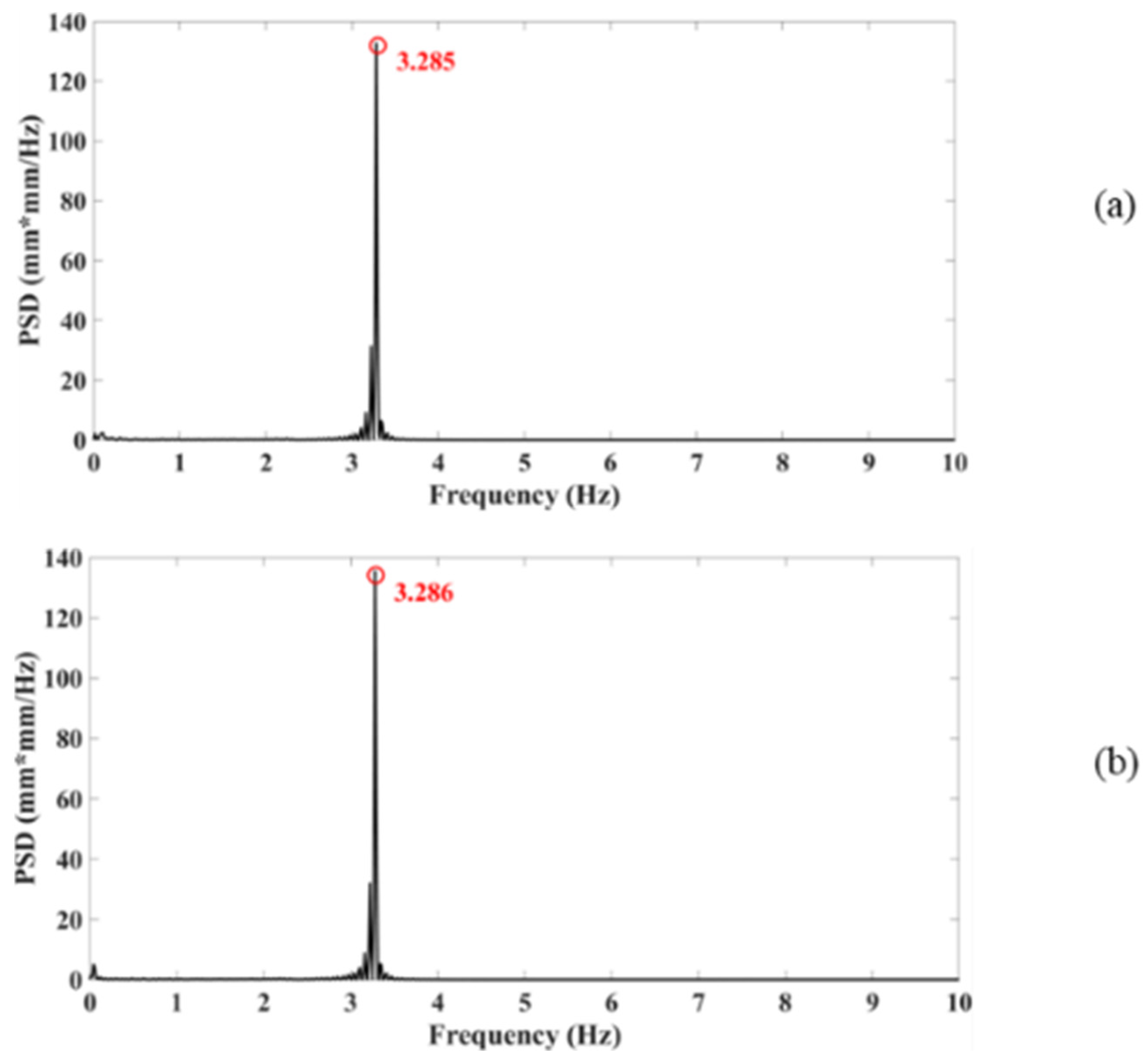
The above displacement signals in Figure 15 are processed into PSD curves, as shown in Figure 16. The natural frequencies extracted for the two displacement signals are 3.285 Hz and 3.286 Hz, respectively, the relative error is 0.04%. It shows that the KLT optical-flow method is feasible to replace DIC to extract the natural frequency of the structure under UAV.

4.3. Comparisons between Fixed Camera and UAV

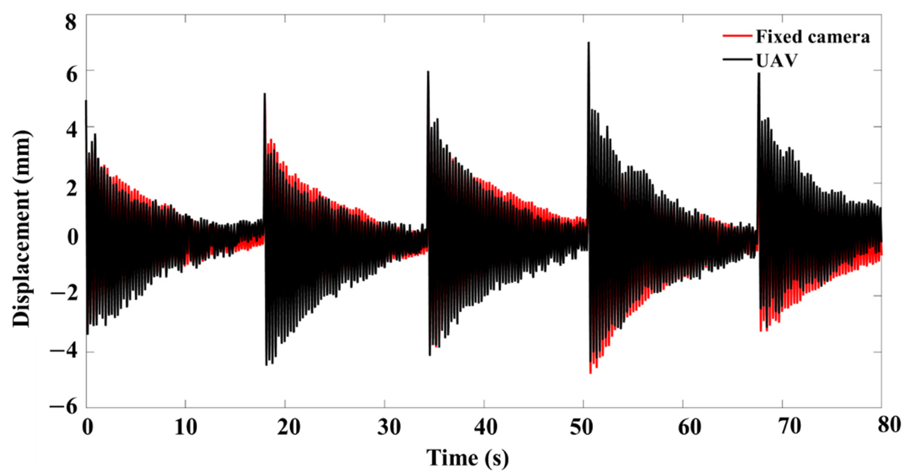
The comparisons of the measurement results of the fixed camera and UAV processed by the KLT optical-flow method are shown in Figure 17, which demonstrates that the corrected displacement curve measured by UAV and the displacement curve measured by fixed camera have very similar free-vibration characteristics. By calculating the time response assurance criterion (TRAC) between the corrected displacement measured by the UAV and the displacement measured by the fixed camera, the correction effect of CNN can be judged [10]. The higher the TRAC, the higher the degree of consistency, and the better the correction effect. The TRAC between displacement measured by the UAV and that measured by the fixed camera is 0.996, which shows their high consistency. Combined with the results of Section 4.2, it can be proved that the displacement of bridge model measured by the UAV combined with the CNN and KLT optical-flow method is reliable.

5. Discussion and Conclusions

5.1. Discussion

5.1.1. Discussion of the Proposed Method

The experimental results show that the displacement of the bridge model measured by a UAV combined with the CNN and KLT optical-flow method is reliable. The displacement signals obtained by the KLT optical-flow method under fixed camera and UAV are more stable than those of DIC, and the extracted structural natural frequency of the KLT optical-flow method is basically consistent with that extracted by DIC, which shows the feasibility of replacing DIC with the KLT optical-flow method in bridge vibration measurement. The difference of the tracking effect between the two methods is mainly caused by the image pyramid of the KLT optical-flow method, which tracks target points at different levels of resolutions of an image to improve tracking accuracy. Under the KLT optical-flow method, the displacement curve measured by UAV combined with CNN is very close to that of the fixed camera, and the natural frequencies obtained by the two methods are basically the same, which shows the feasibility of the method of correcting displacements measured by UAV with CNN proposed in this paper. In the experiment, the 10 reference points are from two different planes (a cardboard and a wall), which shows that the reference points from the same plane are not required for the correction method of this paper, unlike other correction methods. That is one of the highlights of the method proposed in this paper. Moreover, in order to ensure the assumption of constant brightness of the KLT optical-flow method, the measurement can be carried out on cloudy days or when the light condition is stable. Since the measurement duration of the proposed method is about 10 min, the measurement time needs to be determined according to the actual situation.

5.1.2. Follow-Up Study

Although impressive results were obtained in this paper, there are still some problems that need follow-up research:

• The reference point is an important part of the correction method proposed in this paper, so its influence on the correction effect will be studied in the follow-up.
• There may be many influencing factors of accuracy of the proposed method in the actual bridge measurement, such as the wind condition and the actual measurement distance; therefore, the method in this paper will be verified in combination with the actual bridge-measurement results in the follow-up.

5.2. Conclusions

In this paper, a measurement method of bridge vibration by UAVs based on a CNN and KLT optical-flow method is proposed. The effectiveness of the UAV measurement results corrected by a CNN is validated by comparing them with the measurement results of a fixed camera, and the measurement results of DIC are taken as a reference to prove that the KLT optical-flow method is feasible to replace DIC in bridge vibration measurement.

As most of actual bridges cross rivers or valleys, which causes great inconvenience to the measurement, the method introduced in this paper has great prospects in measuring bridge vibration from the perspective of feasibility and accuracy.

References

- Xi, R.; Jiang, W.; Meng, X.; Chen, H.; Chen, Q. Bridge monitoring using BDS-RTK and GPS-RTK techniques. Measurement 2018, 120, 128–139. [Google Scholar] [CrossRef]
- Siringoringo, D.M.; Fujino, Y. Noncontact Operational Modal Analysis of Structural Members by Laser Doppler Vibrometer. Comput. Aided Civ. Infrastruct. Eng. 2010, 24, 249–265. [Google Scholar] [CrossRef]
- Park, K.T.; Kim, S.H.; Park, H.S.; Lee, K.W. The determination of bridge displacement using measured acceleration. Eng. Struct. 2005, 27, 371–378. [Google Scholar] [CrossRef]
- Kovačič, B.; Kamnik, R.; Štrukelj, A.; Vatin, N. Processing of Signals Produced by Strain Gauges in Testing Measurements of the Bridges. Procedia Eng. 2015, 117, 795–801. [Google Scholar] [CrossRef] [Green Version]
- Yi, T.H.; Li, H.N.; Gu, M. Experimental assessment of high-rate GPS receivers for deformation monitoring of bridge. Meas. J. Int. Meas. Confed. 2013, 46, 420–432. [Google Scholar] [CrossRef]
- Reu, P.L.; Rohe, D.P.; Jacobs, L.D. Comparison of DIC and LDV for practical vibration and modal measurements. Mech. Syst. Signal Process. 2017, 86, 2–16. [Google Scholar] [CrossRef] [Green Version]
- Pjsa, B.; Fb, B.; Plc, D.; Pjt, B.; Pmgpm, B. Experimental measurement of bridge deflection using Digital Image Correlation—ScienceDirect. Procedia Struct. Integr. 2019, 17, 806–811. [Google Scholar]
- Chen, G.; Wu, Z.; Gong, C.; Zhang, J.; Sun, X. DIC-Based Operational Modal Analysis of Bridges. Adv. Civ. Eng. 2021, 2021, 6694790. [Google Scholar] [CrossRef]
- Yoneyama, S. Basic principle of digital image correlation for in-plane displacement and strain measurement. Adv. Compos. Mater. 2015, 25, 1–19. [Google Scholar] [CrossRef]
- Chen, G.; Liang, Q.; Zhong, W.; Gao, X.; Cui, F. Homography-based measurement of bridge vibration using UAV and DIC method. Measurement 2020, 170, 108683. [Google Scholar] [CrossRef]
- Deng, G.; Zhou, Z.; Shao, S.; Chu, X.; Jian, C. A Novel Dense Full-Field Displacement Monitoring Method Based on Image Sequences and Optical Flow Algorithm. Appl. Sci. 2020, 10, 2118. [Google Scholar] [CrossRef] [Green Version]
- Zhu, J.; Lu, Z.; Zhang, C. A marker-free method for structural dynamic displacement measurement based on optical flow. Struct. Infrastruct. Eng. 2020, 18, 84–96. [Google Scholar] [CrossRef]
- Shi, J.; Tomasi, C. Good Features to Track. In Proceedings of the Proceedings/CVPR, IEEE Computer Society Conference on Computer Vision and Pattern Recognition, San Francisco, CA, USA, 6 August 2002; Volume 600, pp. 593–600. [Google Scholar]
- Lucas, B.D. An Iterative Image Registration Technique with an Application to Stereo Vision (DARPA). In Proceedings of the 7th International Joint Conference on Artificial Intelligence, Vancouver, BC, Canada, 24–28 August 1981; Volume 81, pp. 674–679. [Google Scholar]
- Review, B. The Perception of the Visual Worldby James J. Gibson. J. Philos. 1951, 48, 788–789. [Google Scholar]
- Liu, F.; Yundong, W.U.; Cai, G.; Chen, S.; Science, S.O.; University, J. Research of Feature Point Tracking Algorithm for UAV Video Image Based on KLT. J. Jimei Univ. 2017, 22, 73–80. [Google Scholar]
- Reagan, D.; Sabato, A.; Niezrecki, C. Feasibility of using digital image correlation for unmanned aerial vehicle structural health monitoring of bridges. Struct. Health Monit. 2018, 17, 1056–1072. [Google Scholar] [CrossRef]
- Ellenberg, A.; Kontsos, A.; Moon, F.; Bartoli, I. Bridge related damage quantification using unmanned aerial vehicle imagery. Struct. Control Health Monit. 2016, 23, 1168–1179. [Google Scholar] [CrossRef]
- Hyunjun, K.; Junhwa, L.; Eunjong, A.; Soojin, C.; Myoungsu, S.; Sung-Han, S. Concrete Crack Identification Using a UAV Incorporating Hybrid Image Processing. Sensors 2017, 17, 2052. [Google Scholar]
- Yoon, H.; Shin, J.; Spencer, B.F. Structural Displacement Measurement Using an Unmanned Aerial System. Comput. Aided Civ. Infrastruct. Eng. 2018, 33, 183–192. [Google Scholar] [CrossRef]
- Mandirola, M.; Casarotti, C.; Peloso, S.; Lanese, I.; Brunesi, E.; Senaldi, I. Use of UAS for damage inspection and assessment of bridge infrastructures. Int. J. Disaster Risk Reduct. 2022, 72, 102824. [Google Scholar] [CrossRef]
- Dong, C.Z.; Bas, S.; Catbas, N. A completely non-contact recognition system for bridge unit influence line using portable cameras and computer vision. Smart Struct. Syst. 2019, 24, 617–630. [Google Scholar]
- Yoneyama, S.; Ueda, H. Bridge Deflection Measurement Using Digital Image Correlation with Camera Movement Correction. Mater. Trans. 2012, 53, 285–290. [Google Scholar] [CrossRef] [Green Version]
- Zhu, X.; Chen, Z.; Tang, C.; Mi, Q.; Yan, X. Application of two oriented partial differential equation filtering models on speckle fringes with poor quality and their numerically fast algorithms. Appl. Opt. 2013, 52, 1814–1823. [Google Scholar] [CrossRef] [PubMed]
- Zhang, J.; Wu, Z.; Chen, G.; Liang, Q. Comparisons of Differential Filtering and Homography Transformation in Modal Parameter Identification from UAV Measurement. Sensors 2021, 21, 5664. [Google Scholar] [CrossRef] [PubMed]
- Zhang, Z. A Flexible New Technique for Camera Calibration. IEEE Trans. Pattern Anal. Mach. Intell. 2000, 22, 1330–1334. [Google Scholar] [CrossRef] [Green Version]
- Wu, Z.; Chen, G.; Ding, Q.; Yuan, B.; Yang, X. Three-Dimensional Reconstruction-Based Vibration Measurement of Bridge Model Using UAVs. Appl. Sci. 2021, 11, 5111. [Google Scholar] [CrossRef]
- Ruian, L.; Nan, L.; Beibei, Z.; Tingting, C.; Ninghao, Y. Geometry correction Algorithm for UAV Remote Sensing Image Based on Improved Neural Network. IOP Conf. 2018, 322, 072002. [Google Scholar]
- Weng, Y.; Shan, J.; Lu, Z.; Lu, X.; Spencer, B.F. Homography-based structural displacement measurement for large structures using unmanned aerial vehicles. Comput. Aided Civ. Infrastruct. Eng. 2021, 36, 1114–1128. [Google Scholar] [CrossRef]
- Brownjohn, J.; Magalhaes, F.; Caetano, E.; Cunha, A. Ambient vibration re-testing and operational modal analysis of the Humber Bridge. Eng. Struct. 2010, 32, 2003–2018. [Google Scholar] [CrossRef] [Green Version]
- Yan, W.J.; Ren, W.X. An Enhanced Power Spectral Density Transmissibility (EPSDT) approach for operational modal analysis: Theoretical and experimental investigation. Eng. Struct. 2015, 102, 108–119. [Google Scholar] [CrossRef]
- Bouguet, J.Y. Pyramidal implementation of the Lucas Kanade feature tracker. Intel Corp. Microprocess. Res. Labs 2000. Available online: http://citeseerx.ist.psu.edu/viewdoc/summary?doi=10.1.1.185.585 (accessed on 25 April 2022).
- Sutton, M.A.; Cheng, M.; Peters, W.H.; Chao, Y.J.; Mcneill, S.R. Application of an optimized digital correlation method to planar deformation analysis. Image Vis. Comput. 1986, 4, 143–150. [Google Scholar] [CrossRef]
- Hubel, D.H.; Wiesel, T.N. Receptive fields, binocular interaction and functional architecture in the cat’s visual cortex. J. Physiol. 1962, 160, 106–154. [Google Scholar] [CrossRef] [PubMed]
- Lecun, Y.; Bottou, L. Gradient-based learning applied to document recognition. Proc. IEEE 1998, 86, 2278–2324. [Google Scholar] [CrossRef] [Green Version]
- De Vriendt, C.; Guillaume, P. The use of transmissibility measurements in output-only modal analysis. Mech. Syst. Signal Process. 2007, 21, 2689–2696. [Google Scholar] [CrossRef]
- Yan, W.J.; Ren, W.X. Operational Modal Parameter Identification from Power Spectrum Density Transmissibility. Comput.-Aided Civ. Infrastruct. Eng. 2012, 27, 202–217. [Google Scholar] [CrossRef]
- Cleveland, W.S. LOWESS: A Program for Smoothing Scatterplots by Robust Locally Weighted Regression. Am. Stat. 1981, 35, 54. [Google Scholar] [CrossRef]
- Margaliot, M.; Hespanha, J.P. Root-mean-square gains of switched linear systems: A variational approach. Automatica 2008, 44, 2398–2402. [Google Scholar] [CrossRef] [Green Version]
Figure 1.
Technical flowchart.
Figure 2.
Motion of points.
Figure 3.
Image pyramid.
Figure 4.
Principle of DIC method.
Figure 5.
Convolution process.
Figure 6.
Architecture of the CNN.
Figure 7.
Experimental model: (a) bridge model; (b) model node; (c) hollow round bar; (d) bolt-connecting balls.
Figure 8.
Image-acquisition equipment: (a) fixed camera; (b) UAV.
Figure 9.
Reference points and experimental layout: (a) reference points; (b) experimental layout.
Figure 10.
Process of displacement correction by CNN.
Figure 11.
Measurement results of vibration model with fixed camera: (a) results of DIC; (b) results of KLT optical-flow method.
Figure 12.
Displacements of the static point obtained by the DIC and KLT optical-flow method.
Figure 13.
PSD obtained by DIC and KLT optical-flow method: (a) results of DIC; (b) results of KLT optical-flow method.
Figure 14.
Uncorrected displacement measured by UAV and false displacement obtained by CNN: (a) results of DIC; (b) results of KLT optical-flow method.
Figure 15.
Comparisons of correction effect of CNN: (a) results of DIC; (b) results of KLT optical-flow method; (c) comparisons.
Figure 16.
PSD measured by UAV: (a) results obtained by DIC; (b) results obtained by KLT.
Figure 17.
Comparisons of results of fixed camera and UAV under KLT optical-flow method.
Publisher’s Note: MDPI stays neutral with regard to jurisdictional claims in published maps and institutional affiliations. |
© 2022 by the authors. Licensee MDPI, Basel, Switzerland. This article is an open access article distributed under the terms and conditions of the Creative Commons Attribution (CC BY) license (https://creativecommons.org/licenses/by/4.0/).
Share and Cite
MDPI and ACS Style
Yan, Z.; Jin, Z.; Teng, S.; Chen, G.; Bassir, D. Measurement of Bridge Vibration by UAVs Combined with CNN and KLT Optical-Flow Method. Appl. Sci. 2022, 12, 5181. https://0-doi-org.brum.beds.ac.uk/10.3390/app12105181
AMA Style
Yan Z, Jin Z, Teng S, Chen G, Bassir D. Measurement of Bridge Vibration by UAVs Combined with CNN and KLT Optical-Flow Method. Applied Sciences. 2022; 12(10):5181. https://0-doi-org.brum.beds.ac.uk/10.3390/app12105181
Chicago/Turabian StyleYan, Zhaocheng, Zihan Jin, Shuai Teng, Gongfa Chen, and David Bassir. 2022. "Measurement of Bridge Vibration by UAVs Combined with CNN and KLT Optical-Flow Method" Applied Sciences 12, no. 10: 5181. https://0-doi-org.brum.beds.ac.uk/10.3390/app12105181
Note that from the first issue of 2016, this journal uses article numbers instead of page numbers. See further details here.