
An Experimental Ultrasound Database for Tomographic Imaging


Centro Direzionale, University of Napoli Parthenope, 80143 Napoli, Italy
*
Author to whom correspondence should be addressed.
Appl. Sci. 2022, 12(10), 5192; https://0-doi-org.brum.beds.ac.uk/10.3390/app12105192
Submission received: 28 March 2022
/
Revised: 12 May 2022
/
Accepted: 14 May 2022
/
Published: 20 May 2022
(This article belongs to the Special Issue Ultrasound Technology in Industry and Medicine)
Abstract
:In the framework of non-destructive testing and imaging, ultrasound tomography can have an important role in several applications, especially in the biomedical field. The motivation beyond the use of this imaging technique lies in the possibility of obtaining quantitative imaging which is also operator-independent, conversely to conventional approaches. Thus, the need for public data sets for testing inverse scattering approaches is always persisting. To this aim, this paper introduces an experimental multiple-input-multiple-output ultrasound tomographic database whose acquisitions were performed by an air-matched in-house system designed and built by the Authors. The proposed database provides several cases with single and multiple objects of different shapes, sizes, and materials, to be imaged in laboratory-controlled conditions. Therefore, these scenarios can represent interesting options for the preliminary testing of tomographic ultrasound imaging approaches.
1. Introduction
Ultrasound imaging is one of the most adopted imaging modalities for non-destructive testing and diagnostics [1]. Nevertheless, conventional approaches suffer from some limitations, such as the operator-dependent feature and the presence of speckles which degrades the quality of the images, thus requiring the use of proper filtering strategies [2,3,4]. In this framework and to provide a quantitative, operator-independent imaging modality, ultrasound tomography has achieved significant interest.
Ultrasound tomography (UST) represents an imaging modality that exploits ultrasound waves to retrieve information about the mechanical properties of objects of interest (OIs). In UST, the pressure fields are measured by ultrasound (US) transducers located outside the OIs to locate and eventually characterize them in terms of density, compressibility and attenuation [5,6,7]. Due to the fact that the data acquisition measures the received voltage at the port of one or more of the receiving transducers to infer the pressure field impinging directly on the sensor, a proper calibration procedure that takes into account the radiation factor, implicitly or explicitly, is required to perform the imaging.
More in detail, the idea of arranging ultrasound transducers around the imaged objects in a fixed setup goes back to the early 1980s [8]. Since then, several scientists have been working on UST [9,10,11,12,13], and most of this work is focused on noninvasive medical imaging, especially for breast cancer applications [14,15,16,17], in which field considerable tumor detection and characterization improvements can be appreciated if UST is applied in combination with other imaging approaches [18,19,20,21].
To perform the data acquisition in UST, two main options are available: the first one exploits the use of a single transmitter-receiver pair that mechanically moves around the investigation region, while the second option carries out the data collection via adopting more transmitters and receivers physically located around the area of interest. This latter option, which is also known in communication technologies as the multiple-input-multiple-output (MIMO) configuration, represents the case considered in the proposed manuscript. The aim of the work is to face the common issue in the inverse scattering community of the lack of experimental US tomographic scattering data. The quest for experimental data was already partially satisfied in different contexts [22,23,24,25], in which cases the angular diversity information is collected via mechanical movements of the bistatic pair of transmitter and receiver around the OIs. However, there are several applications for which scattering data are better collected with mechanically static systems, such as biomedical imaging and nondestructive testing.
Despite the experimental data sets available for ultrasound systems, most of them focus on complex scenarios more suitable for denoising and image processing purposes rather than for testing tomographic coherent imaging approaches in relatively simple laboratory-controlled conditions.
Thus, with the goal of stimulating the research for both imaging and calibration issues, this work presents a tomographic database of ultrasound scattering measurements. The acquisitions were performed by adopting an in-house imaging system which is described in Section 2. In the following, different scenarios are considered with an increased level of complexity to allow the performance testing of both image formation and detection algorithms.
2. Experimental Ultrasound System
In this section, the proposed UST system, that was designed, built, and tested at the University of Naples Parthenope, is presented. The overall system, which is shown in Figure 1, was intended for the acquisition of a single slice of the investigation domain and consists of three main components:
- a circular wooden ring hosting twenty-two US transducers (both transmitters and receivers);
- a signal generator (Agilent Technologies, model 33220A) for the transmitters excitation;
- an analog-to-digital converter (National Instrument, 6363 DAQ USB X Series);
- a standard laptop to control the acquisitions and to perform the processing.
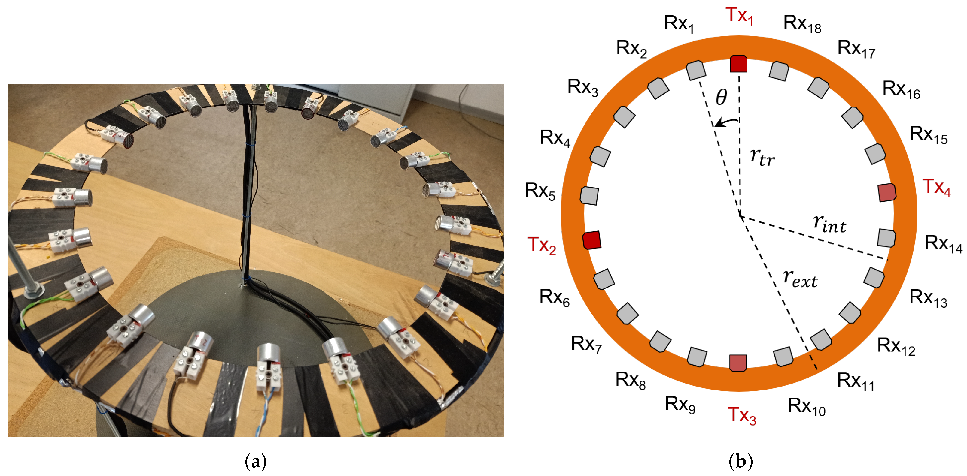
The imaging region is surrounded by twenty-two transducers (i.e., four transmitters and eighteen receivers), approximately equally spaced on a wooden circular ring as shown in Figure 2. The circular wooden ring on which the transducers are located is hung by means of three thin metallic bars (Figure 2a). The height of the imaging plane and the presence of an absorbing element on the floor of the system reduce the presence of clutter considerably, allowing good isolation of the back-scattered signal related to the OIs.
The internal and external radii of the wooden ring are equal to cm and cm, respectively, while the distance of each transducer from the centre of the investigation area is approximately cm. The angular distance between two consecutive transducers is about .
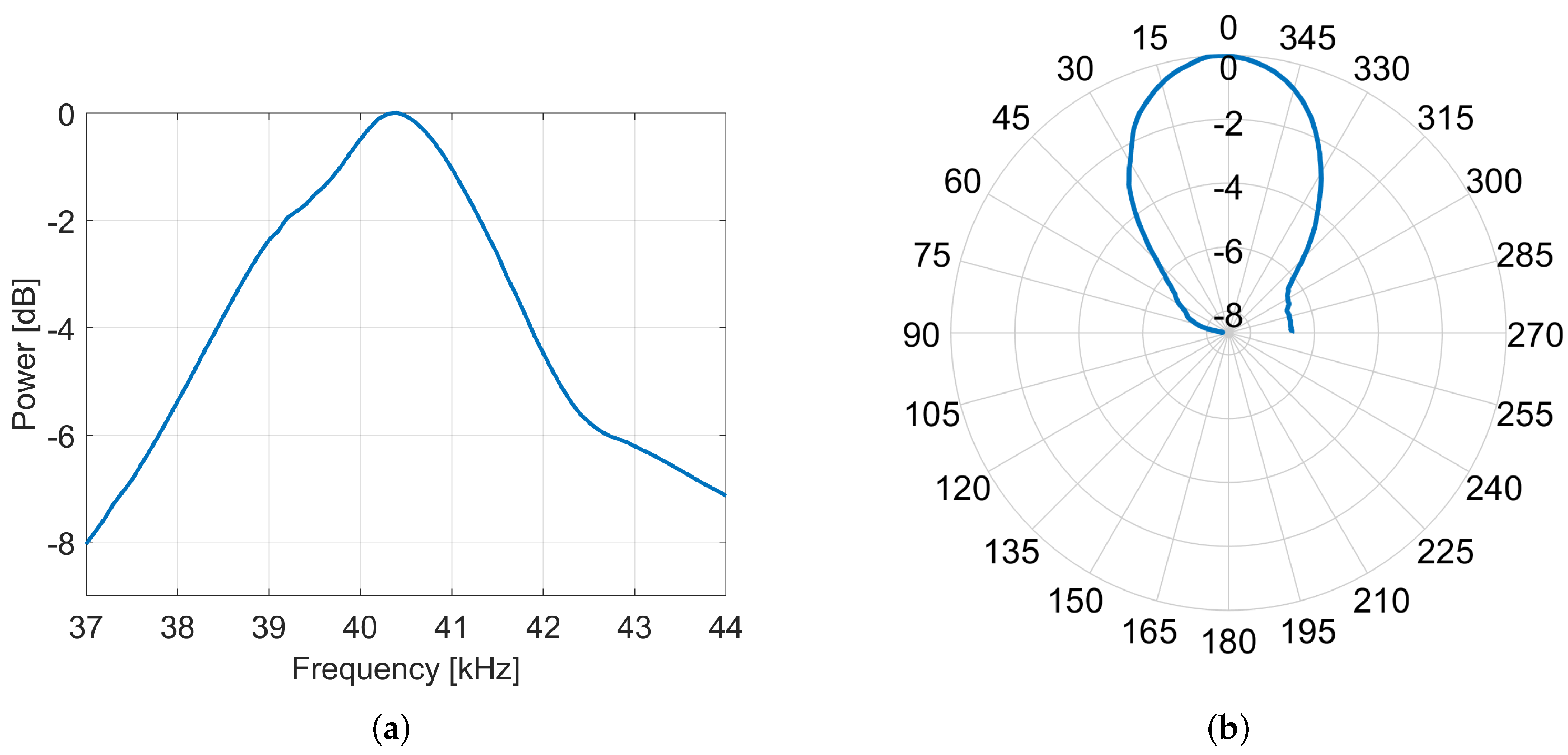
As detailed in Figure 2b, the four transmitters are located at the cardinal points in a slightly asymmetrical position, i.e., two consecutive transmitters might be separated by either 4 or 5 receivers, according to the considered angular sector. The transducers used as transmitters and receivers are, respectively, the 40LT16 and 40LR16 both manufactured by SensComp. Both of these types of sensors have a central working frequency of 40 kHz and narrow bandwidth of approximately 2 kHz. At the central frequency of 40 kHz, the corresponding wavelength is approximately 8.5 mm. The bandwidth was experimentally measured and decreases to a −8 dB power-level difference as proved by Figure 3a. In the following, an operational bandwidth of 4 kHz ( kHz) will be considered for the acquisition protocol. Regarding the beam angle, it extends for approximately at −3 dB both in the vertical as well as horizontal planes (Figure 3b).
The region of interest (ROI), i.e., the scanning area in which the objects are located, coincides with the central area of the circular array.
The received US waves are converted into electric signals by 40LR16 transducers and then digitalized by an analog-to-digital converter manufactured by National Instruments. Once acquired, the beat signals are computed to demodulate the signals. Both acquisition and beat-signal extraction steps are computed via a Matlab script (available in the Supplementary Material).
3. Data Acquisition Protocol
The proposed work aims to create a database of measured US scattered pressure fields for tomographic inversion purposes and to provide the scientific imaging community the opportunity to test the resolution capability of their approaches in some laboratory-controlled conditions with different levels of complexity.
Therefore, in the present study, both the fields with and without the OIs located in the investigation area are collected, named and , respectively. These two types of measures are performed in order to allow the evaluation of the scattered field by means of a subtraction operation, i.e., .
The acquisition protocol consists of a set of measurements per each scenario. More in detail, a stepped-frequency continuous-wave monochromatic signal was adopted as a source with a total of 41 equally-spaced frequency points in the range kHz with a sampling frequency of 500 kHz and a sixteen-bit precision. It is worth noting that the frequency step used to sample the considered band is equal to 100 Hz. Thus, adopting this choice guarantees a sufficiently large unambiguous distance, which for the considered settings is approximately equal to 1.71 meters, which is suitable for the proposed setup.
The sinusoidal pulse used as an active signal has a duration of 20 ms per frequency and the procedure is repeated per each of the 4 transmitters of the circular array. Regarding the acquisitions, they are not simultaneous, but sequential, i.e., at each frequency one single transmitter is active and then one receiving channel acquires the data. In order to avoid transitional effects, the acquisition of each frequency includes a pause to ensure the collection of steady-state data. After that, the receiving operation is repeated and carried out sequentially for each receiving transducer, and then per each transmitter. It is worth noting that the use of a 20-ms-length window per frequency ensures that the side lobes of sinc replicas that are in the band of interest are 90 dB lower than the power peak, making any low-pass filter unnecessary. The final time to complete the acquisition of each scenario (i.e., 41 frequency points, 4 views, 18 measures) is about 20 min.
After the acquisition, the signal is filtered in the range kHz to reduce the effect of noise, and the mean beat signal is computed. Finally, due to the considered static scenes, an average value is determined for the whole observation window. Thus, at each frequency, a single complex value is obtained per transmitter-receiver pair.
4. Data Set Description
The objects which compose the database are homogeneous objects of different sizes (0.7–5.0 cm), shapes (spheres and cubes), and materials (wooden, styrofoam, cork). A picture of the targets adopted for the measurement campaign is shown in Figure 4 with further details reported in Table 1. The reader can refers to [26] for the evaluation of the target strength.
The imaging scenario was obtained by placing the objects inside the imaging plane. As support for the targets, some nylon wires were used to hang them in the central area in the same plane the transducers are. The acquisition of the scenes is static, thus the objects are stable and fixed during the measurements.
Basically, the data set is composed of different scenarios with different targets and arrangements. More in detail, the scenarios are illustrated in Figure 5, Figure 6, Figure 7 and Figure 8 and organized according to the following scheme:
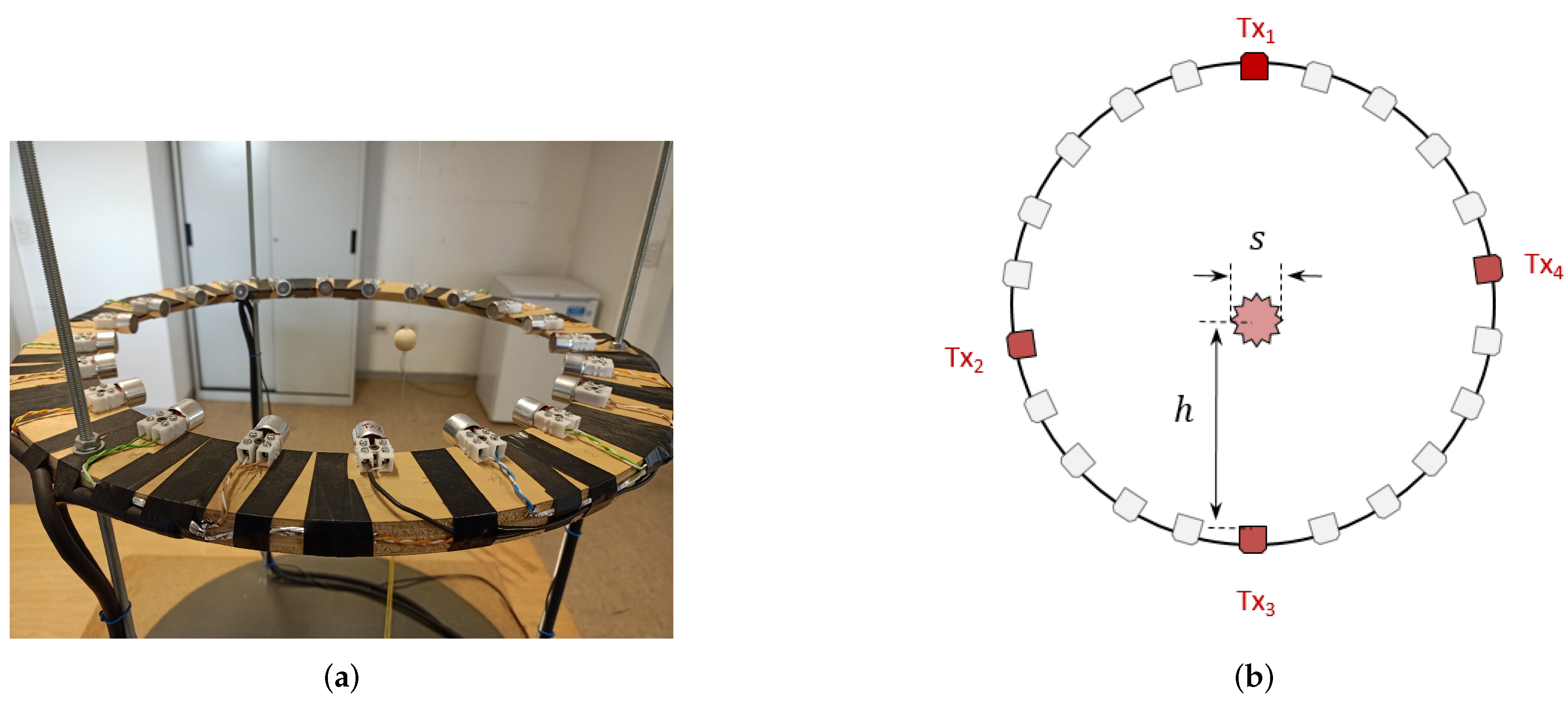
- Scenario 1: A single object of different shape, size, and materialIn this set of measurements, the acquisition of a single object of various shapes, sizes, and materials is considered, as illustrated in Figure 5. The types of objects are briefly summarised in Table 1, which provides the main details. In all these measurements, for a total of 13 acquisitions, the position of the object remains fixed and only its size and material change, as detailed in Table 2.
- Scenario 2: two wooden spheres of equal size
- Scenario 3: Two objects of different size, shape, and material
- Scenario 4: three objects
The data are stored in “.mat” format and named with the following criterion: “scenario-X-YY.mat”, with the number “X” referring to the scenario ID and with the number “YY” referring to the acquisition number. Thus, for instance, if the considered file is named “scenario-2-07.mat”, this file contains the data related to scenario 2 and set ID number 07. Each of these files contains different variables, “u-obj” and “u-emp” refer to the acquisition performed with target(s) inside the investigation domain and without any object, respectively. Furthermore, “r” is the radius of the measurement curve, “rx-angles” and “tx-angles” represents the angular position of the receivers and the transmitters, respectively, “f”, contains the values of the operative frequencies. The remaining variables, i.e., “h”, “s” and “objects-type”, are specific per each scenario (see Figure 5, Figure 6, Figure 7 and Figure 8 and Table 2, Table 3, Table 4 and Table 5).
Regarding the data structure, each variable consists of a three-index matrix: the first two dimensions identify the receiver and transmitter ID, respectively, with sorting as reported in Figure 2b, while the last dimension refers to the number of adopted frequencies. Thus, the size of each matrix variable is . The data sets and the related acquisition code are available in the Supplementary Material of the paper.
Finally, a numerical validation of the proposed experimental tomographic system is carried out via a comparison with simplified two-dimensional (2D) numerical simulations by using the K-Wave MATLAB toolbox [27]. K-Wave is a framework designed to make realistic photoacoustic analyses. The forward problem is solved via k-space pseudo-spectral time-domain computations for solving coupled first-order acoustic equations for both homogeneous and heterogeneous media in one, two, and three dimensions.
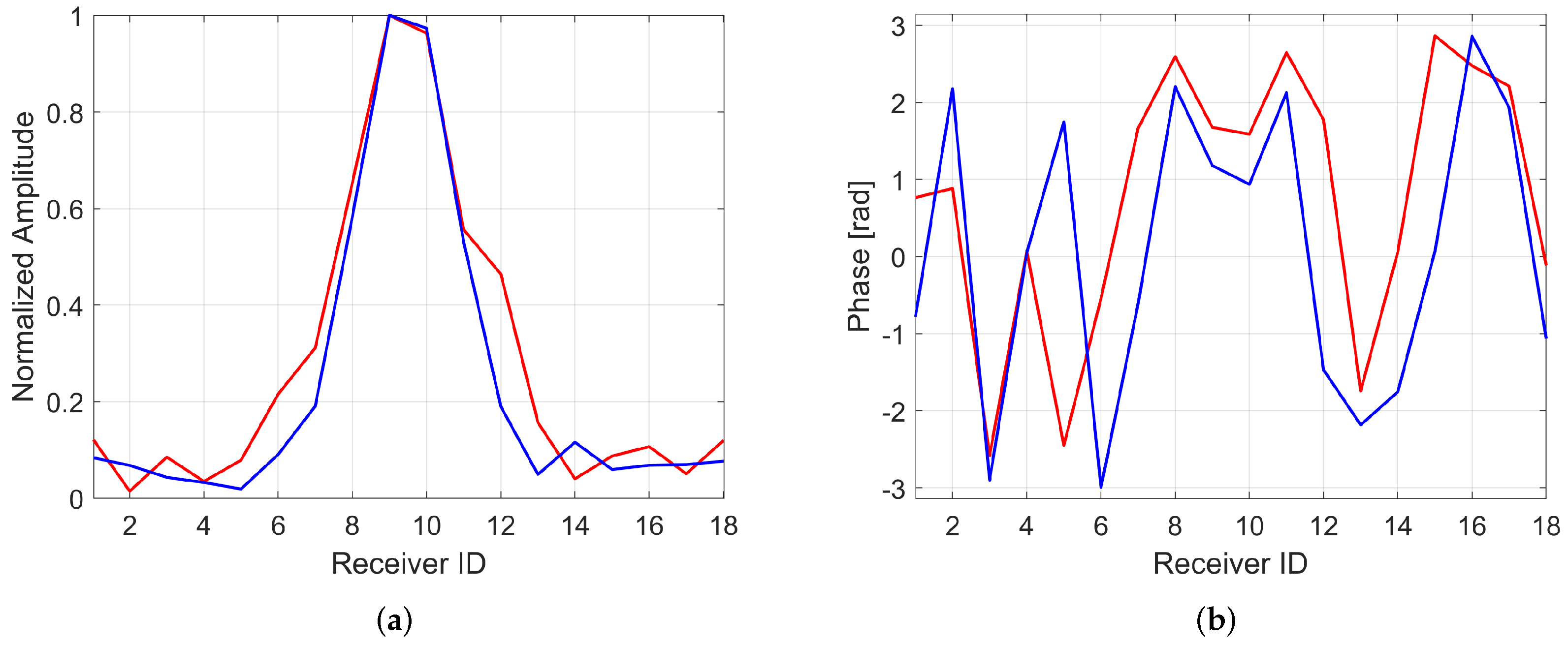
Figure 9 reports a comparison between the signal measured by the proposed system (single view) with a cylindrical 4-mm-diameter metallic target located inside the investigation domain and a simplified 2D numerical simulation performed by the K-Wave toolbox with the sensors’ positions assumed equally-spaced in angle along the measurement circle. It can be noticed that there is a good match between the measured field and the numerical simulation, even though some small differences in amplitude and phase are present. In this regard, it is worth noting that a very good match can be observed for transducers with higher SNR (i.e., from 6 to 14) both in amplitude and phase. Moreover, for these transducers the phase difference is approximately 0.5 radians, which corresponds to a difference in space of about 0.3 mm, to be ascribed to a positioning error for the target. These differences can be ascribed to a few causes, such as the simplified 2D numerical model adopted for the comparison, which is still a full-wave model, as well as the precision in locating the small, simulated target in the right place to agree with the correct location of the metallic bar used for the real measurement, but also the approximation in the radiation pattern which is here assumed 2D for the sake of ease. The Matlab code related to the numerical simulation of Figure 9 is reported in the Supplementary Material.
5. Conclusions
In this paper, an experimental tomographic imaging database for ultrasound tomography designed and built at the University of Naples Parthenope was presented. The proposed US database represents an interesting laboratory-controlled situation for the testing of imaging and localization approaches and their performance, which is paramount prior to their use in complex and realistic scenarios. This work tries to meet the impelling need of the scientific community for testing inverse scattering approaches.
In this work, the acquisition was performed in an air-matched in-house system considering several scenarios with single and multiple objects of different shapes, sizes, and materials. The measures were performed at different equally-spaced frequencies in the range [38, 42] kHz and, per acquisition, both the data collected in the presence and absence of the targets were collected and stored in mat variables which are available in the Supplementary Material of the paper.
Future work will be focused on the extension of the considered system, properly re-designed and re-scaled, to the case of water-matched UST in the framework of biomedical applications.
Supplementary Materials
The following are available online at https://0-www-mdpi-com.brum.beds.ac.uk/article/10.3390/app12105192/s1.
Author Contributions
Conceptualization, M.A. and F.B.; resources, A.G. and G.G.; methodology, S.F. and M.A.; validation, S.F. and M.A.; writing—review and editing, S.F., M.A., A.G., G.G., and F.B.; visualization, S.F. and M.A.; supervision, F.B. All authors have read and agreed to the published version of the manuscript.
Funding
This research received no external funding.
Institutional Review Board Statement
Not applicable.
Informed Consent Statement
Not applicable.
Data Availability Statement
Data available in Supplementary Material.
Conflicts of Interest
The authors declare no conflict of interest.
Abbreviations
The following abbreviations are used in this manuscript:
| MIMO | multiple-input-multiple-output |
| OIs | objects of interest |
| US | ultrasound |
| UST | ultrasound tomography |
References
- Sanches, J.M.; Laine, A.F.; Suri, J.S. Ultrasound Imaging; Springer: Berlin/Heidelberg, Germany, 2012. [Google Scholar]
- Joel, T.; Sivakumar, R. Despeckling of ultrasound medical images: A survey. J. Image Graph. 2013, 1, 161–165. [Google Scholar] [CrossRef]
- Yahya, N.; Kamel, N.S.; Malik, A.S. Subspace-based technique for speckle noise reduction in SAR images. IEEE Trans. Geosci. Remote Sens. 2014, 52, 6257–6271. [Google Scholar] [CrossRef]
- Ambrosanio, M.; Baselice, F.; Ferraioli, G.; Pascazio, V. Ultrasound despeckling based on non local means. In EMBEC & NBC 2017; Springer: Berlin/Heidelberg, Germany, 2017; pp. 109–112. [Google Scholar]
- Gemmeke, H.; Ruiter, N.V. 3D ultrasound computer tomography for medical imaging. Nucl. Instrum. Methods Phys. Res. Sect. Accel. Spectrom. Detect. Assoc. Equip. 2007, 580, 1057–1065. [Google Scholar] [CrossRef]
- Korta Martiartu, N.; Boehm, C.; Hapla, V.; Maurer, H.; Balic, I.J.; Fichtner, A. Optimal experimental design for joint reflection-transmission ultrasound breast imaging: From ray-to wave-based methods. J. Acoust. Soc. Am. 2019, 146, 1252–1264. [Google Scholar] [CrossRef]
- Goncharsky, A.V.; Romanov, S.Y.; Seryozhnikov, S.Y. Low-frequency ultrasonic tomography: Mathematical methods and experimental results. Mosc. Univ. Phys. Bull. 2019, 74, 43–51. [Google Scholar] [CrossRef]
- Greenleaf, J.F.; Bahn, R.C. Clinical imaging with transmissive ultrasonic computerized tomography. IEEE Trans. Biomed. Eng. 1981, 2, 177–185. [Google Scholar] [CrossRef]
- Fink, M. Time reversal of ultrasonic fields. i. basic principles. IEEE Trans. Ultrason. Ferroelectr. Freq. Control. 1992, 39, 555–566. [Google Scholar] [CrossRef]
- Dong, C.; Jin, Y.; Lu, E. Accelerated nonlinear multichannel ultrasonic tomographic imaging using target sparseness. IEEE Trans. Image Process. 2014, 23, 1379–1393. [Google Scholar] [CrossRef]
- Moallemi, N.; Shahbazpanahi, S. A new model for array spatial signature for two-layer imaging with applications to nondestructive testing using ultrasonic arrays. IEEE Trans. Signal Process. 2015, 63, 2464–2475. [Google Scholar] [CrossRef]
- Wiskin, J.; Malik, B.; Borup, D.; Pirshafiey, N.; Klock, J. Full wave 3d inverse scattering transmission ultrasound tomography in the presence of high contrast. Sci. Rep. 2020, 10, 1–14. [Google Scholar] [CrossRef]
- Franceschini, S.; Ambrosanio, M.; Baselice, F.; Pascazio, V. A tomographic multiview-multistatic ultrasound system for biomedical imaging applications. In Proceedings of the 13th International Joint Conference on Biomedical Engineering Systems and Technologies (BIOSTEC 2020)—Volume 1: BIODEVICES, Valletta, Malta, 24–26 February 2020; pp. 274–279. [Google Scholar]
- Yang, M.; Sampson, R.; Wei, S.; Wenisch, T.F.; Chakrabarti, C. Separable beamforming for 3-d medical ultrasound imaging. IEEE Trans. Signal Process. 2014, 63, 279–290. [Google Scholar] [CrossRef]
- Huthwaite, P.; Simonetti, F. High-resolution imaging without iteration: A fast and robust method for breast ultrasound tomography. J. Acoust. Soc. Am. 2011, 130, 1721–1734. [Google Scholar] [CrossRef] [PubMed] [Green Version]
- Sandhu, G.Y.; Li, C.; Roy, O.; Schmidt, S.; Duric, N. Frequency domain ultrasound waveform tomography: Breast imaging using a ring transducer. Phys. Med. Biol. 2015, 60, 5381. [Google Scholar] [CrossRef] [PubMed]
- Mojabi, P.; LoVetri, J. Evaluation of balanced ultrasound breast imaging under three density profile assumptions. IEEE Trans. Comput. Imaging 2017, 3, 864–875. [Google Scholar] [CrossRef]
- Qin, Y.; Rodet, T.; Lambert, M.; Lesselier, D. Joint inversion of electromagnetic and acoustic data with edge-preserving regularization for breast imaging. IEEE Trans. Comput. Imaging 2021, 7, 349–360. [Google Scholar] [CrossRef]
- Qin, Y.; Rodet, T.; Lambert, M.; Lesselier, D. Microwave breast imaging with prior ultrasound information. IEEE Open J. Antennas Propag. 2020, 1, 472–482. [Google Scholar] [CrossRef]
- Abdollahi, N.; Kurrant, D.; Mojabi, P.; Omer, M.; Fear, E.; LoVetri, J. Incorporation of ultrasonic prior information for improving quantitative microwave imaging of breast. IEEE J. Multiscale Multiphys. Comput. Tech. 2019, 4, 98–110. [Google Scholar] [CrossRef]
- Mojabi, P.; LoVetri, J. Experimental evaluation of composite tissue-type ultrasound and microwave imaging. IEEE J. Multiscale Multiphys. Comput. Tech. 2019, 4, 119–132. [Google Scholar] [CrossRef]
- Camacho, J.; Medina, L.; Cruza, J.F.; Moreno, J.M.; Fritsch, C. Multimodal ultrasonic imaging for breast cancer detection. Arch. Acoust. 2012, 37, 253–260. [Google Scholar] [CrossRef]
- González-Salido, N.; Medina, L.; Camacho, J. Full angle spatial compound of arfi images for breast cancer detection. Ultrasonics 2016, 71, 161–171. [Google Scholar] [CrossRef]
- Rodriguez-Molares, A.; Rindal, O.M.H.; Bernard, O.; Nair, A.; Bell, M.A.L.; Liebgott, H.; Austeng, A. The ultrasound toolbox. In Proceedings of the 2017 IEEE International Ultrasonics Symposium (IUS), Washington, DC, USA, 6–9 September 2017; pp. 1–4. [Google Scholar]
- Ruiter, N.V.; Zapf, M.; Hopp, T.; Gemmeke, H.; Van Dongen, K.W. Usct data challenge. In Proceedings of the Medical Imaging 2017: Ultrasonic Imaging and Tomography, Orlando, FL, USA, 15–16 February 2017; Volume 10139, p. 101391N. [Google Scholar]
- Gudra, T.; Opielinski, K.J.; Jankowski, J. Estimation of the variation in target strength of objects in the air. Int. Congr. Ultrason. 2010, 3, 209–215. [Google Scholar] [CrossRef] [Green Version]
- Treeby, B.; Cox, B.T. k-wave: Matlab toolbox for the simulation and reconstruction of photoacoustic wave fields. J. Biomed. Opt. 2010, 15, 021314. [Google Scholar] [CrossRef] [PubMed]
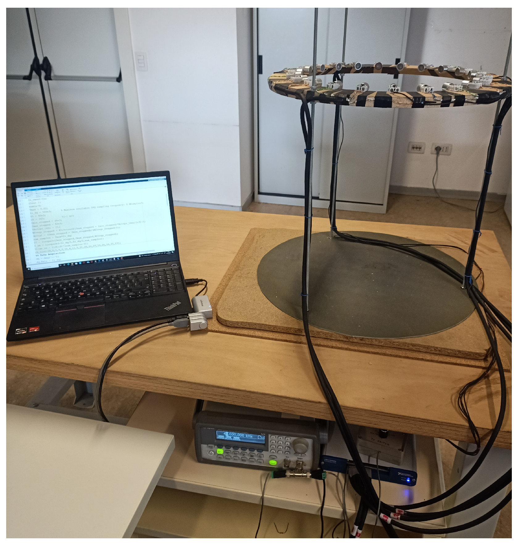
Figure 1.
Picture of the tomographic ultrasound system. The transmitters are connected to the signal generator (bottom left), while the receivers are connected to a data acquisition device (bottom right). The whole acquisition is controlled via a laptop with Matlab software.
Figure 1.
Picture of the tomographic ultrasound system. The transmitters are connected to the signal generator (bottom left), while the receivers are connected to a data acquisition device (bottom right). The whole acquisition is controlled via a laptop with Matlab software.

Figure 2.
(a) Picture of the US transducers circular array and (b) sketch of its arrangement with details about transmitters (in red) and receivers (in grey). The dimensions are: cm, cm, cm and .
Figure 2.
(a) Picture of the US transducers circular array and (b) sketch of its arrangement with details about transmitters (in red) and receivers (in grey). The dimensions are: cm, cm, cm and .

Figure 3.
(a) Transducers frequency response in the band kHz and (b) radiation pattern at the frequency of 40 kHz. The pattern is approximately the same in both horizontal and vertical planes.
Figure 3.
(a) Transducers frequency response in the band kHz and (b) radiation pattern at the frequency of 40 kHz. The pattern is approximately the same in both horizontal and vertical planes.

Figure 4.
Picture of the objects adopted for the measurement campaign. From the top row: circular wooden spheres of different size, styrofoam cubes and spheres, cork cubes.
Figure 4.
Picture of the objects adopted for the measurement campaign. From the top row: circular wooden spheres of different size, styrofoam cubes and spheres, cork cubes.

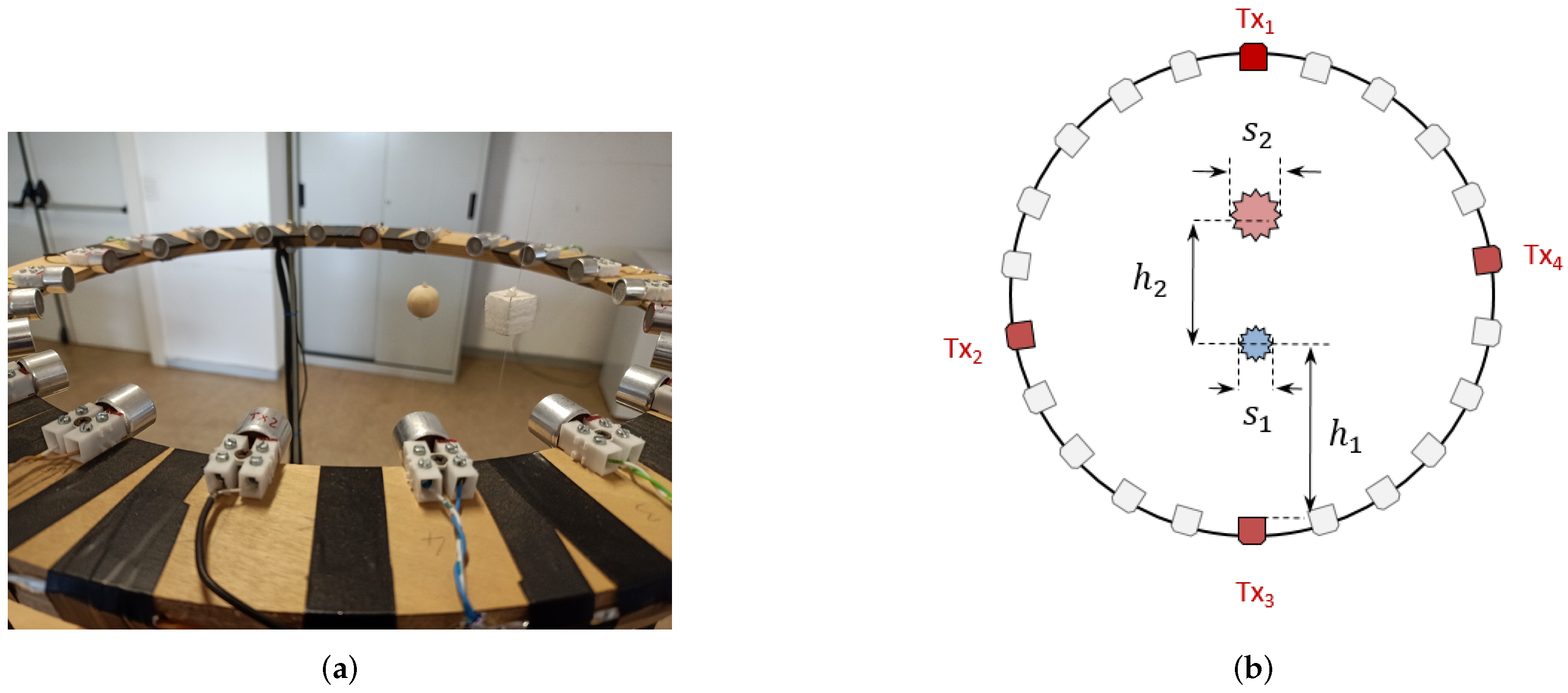
Figure 5.
Scenario 1: single object of different shape, size and material. (a) Picture of an acquisition and (b) its sketch in a two-dimensional plane.
Figure 5.
Scenario 1: single object of different shape, size and material. (a) Picture of an acquisition and (b) its sketch in a two-dimensional plane.

Figure 6.
Scenario 2: two wooden spheres of equal size. (a) Picture of an acquisition and (b) its sketch in a two-dimensional plane.
Figure 6.
Scenario 2: two wooden spheres of equal size. (a) Picture of an acquisition and (b) its sketch in a two-dimensional plane.

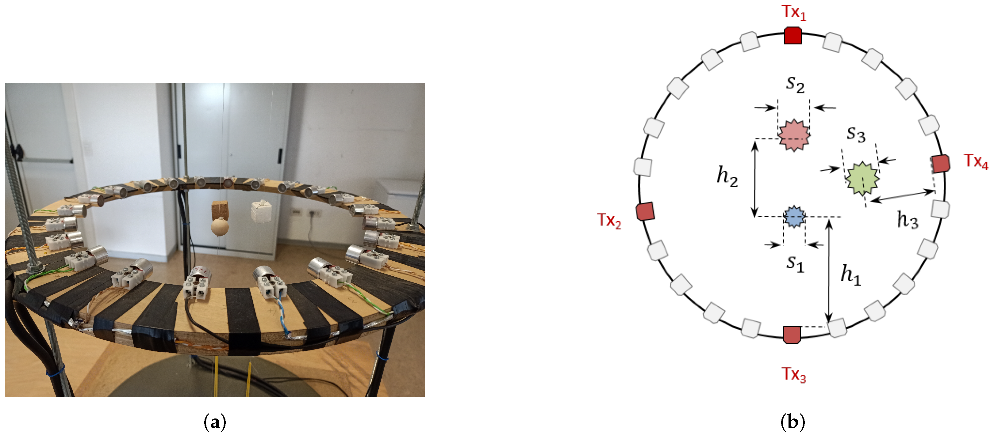
Figure 7.
Scenario 3: two objects of different size, shape and material. (a) Picture of an acquisition and (b) its sketch in a two-dimensional plane.
Figure 7.
Scenario 3: two objects of different size, shape and material. (a) Picture of an acquisition and (b) its sketch in a two-dimensional plane.

Figure 8.
Scenario 4: three objects. (a) Picture of an acquisition and (b) its sketch in a two-dimensional plane.
Figure 8.
Scenario 4: three objects. (a) Picture of an acquisition and (b) its sketch in a two-dimensional plane.

Figure 9.
Comparison between measured (red line) and simulated (blue line) data by K-Wave Matlab toolbox for the amplitude (a) and phase (b) signals.
Figure 9.
Comparison between measured (red line) and simulated (blue line) data by K-Wave Matlab toolbox for the amplitude (a) and phase (b) signals.


Table 1.
Features of the objects involved in the measurement campaign.
| Object | Size (Diameter/Side) [cm] | Shape | Material |
|---|---|---|---|
 | Sphere | Wood | |
 | Sphere | Styrofoam | |
 | Cube | Styrofoam | |
 | Cube | Cork |
Table 2.
Scenario 1: single object of different shape, size and material (Figure 5). The quantity s refers to the diameter for spherical objects and to the side for cubes.
Table 2.
Scenario 1: single object of different shape, size and material (Figure 5). The quantity s refers to the diameter for spherical objects and to the side for cubes.
| Set | Object (  ) ) | h [cm] | s [cm] |
|---|---|---|---|
| 1.01 | | 11 | |
| 1.02 | | 11 | |
| 1.03 | | 11 | |
| 1.04 | | 11 | |
| 1.05 | | 11 | |
| 1.06 | | 11 | |
| 1.07 | | ||
| 1.08 | | ||
| 1.09 | | ||
| 1.10 | | ||
| 1.11 | | 11 | |
| 1.12 | | 11 | |
| 1.13 | | 11 |
Table 3.
Scenario 2: two wooden spheres of equal size (Figure 6).
Table 3.
Scenario 2: two wooden spheres of equal size (Figure 6).
| Set | Object | s [cm] | [cm] | [cm] |
|---|---|---|---|---|
| 2.01 | | 11 | ||
| 2.02 | | 11 | ||
| 2.03 | | 11 | ||
| 2.04 | | 11 | ||
| 2.05 | | 11 | ||
| 2.06 | | 11 | ||
| 2.07 | | 11 | ||
| 2.08 | | 11 |
Table 4.
Scenario 3: two objects of different size, shape and material (Figure 7). The quantity s refers to the diameter for spherical objects and to the side for cubes.
Table 4.
Scenario 3: two objects of different size, shape and material (Figure 7). The quantity s refers to the diameter for spherical objects and to the side for cubes.
| Set | Object 1 ( ) | [cm] | [cm] | Object 2 (  ) ) | [cm] | [cm] |
|---|---|---|---|---|---|---|
| 3.01 | | 11 | | |||
| 3.02 | | 11 | | |||
| 3.03 | | 11 | | |||
| 3.04 | | 11 | | |||
| 3.05 | | 13 | | |||
| 3.06 | | 13 | | |||
| 3.07 | | 13 | | |||
| 3.08 | | 13 | | |||
| 3.09 | | | ||||
| 3.10 | | | ||||
| 3.11 | | | ||||
| 3.12 | | | ||||
| 3.13 | | | ||||
| 3.14 | | | ||||
| 3.15 | | 11 | | |||
| 3.16 | | 11 | | |||
| 3.17 | | 11 | | |||
| 3.18 | | 11 | | |||
| 3.19 | | 11 | | |||
| 3.20 | | 11 | |
Table 5.
Scenario 4: three objects of different size, shape and material (Figure 8). The quantity s refers to the diameter for spherical objects and to the side for cubes.
Table 5.
Scenario 4: three objects of different size, shape and material (Figure 8). The quantity s refers to the diameter for spherical objects and to the side for cubes.
| Set | Object 1 ( ) | [cm] | [cm] | Object 2 ( ) | [cm] | [cm] | Object 3 (  ) ) | [cm] | [cm] |
|---|---|---|---|---|---|---|---|---|---|
| 4.01 | | 10 | | | |||||
| 4.02 | | | | ||||||
| 4.03 | | 18 | | | |||||
| 4.04 | | 14 | | | |||||
| 4.05 | | 14 | | | |||||
| 4.06 | | 14 | | |
Publisher’s Note: MDPI stays neutral with regard to jurisdictional claims in published maps and institutional affiliations. |
© 2022 by the authors. Licensee MDPI, Basel, Switzerland. This article is an open access article distributed under the terms and conditions of the Creative Commons Attribution (CC BY) license (https://creativecommons.org/licenses/by/4.0/).
Share and Cite
MDPI and ACS Style
Franceschini, S.; Ambrosanio, M.; Gifuni, A.; Grassini, G.; Baselice, F. An Experimental Ultrasound Database for Tomographic Imaging. Appl. Sci. 2022, 12, 5192. https://0-doi-org.brum.beds.ac.uk/10.3390/app12105192
AMA Style
Franceschini S, Ambrosanio M, Gifuni A, Grassini G, Baselice F. An Experimental Ultrasound Database for Tomographic Imaging. Applied Sciences. 2022; 12(10):5192. https://0-doi-org.brum.beds.ac.uk/10.3390/app12105192
Chicago/Turabian StyleFranceschini, Stefano, Michele Ambrosanio, Angelo Gifuni, Giuseppe Grassini, and Fabio Baselice. 2022. "An Experimental Ultrasound Database for Tomographic Imaging" Applied Sciences 12, no. 10: 5192. https://0-doi-org.brum.beds.ac.uk/10.3390/app12105192
Note that from the first issue of 2016, this journal uses article numbers instead of page numbers. See further details here.