
Study on Underwater Target Tracking Technology Based on an LSTM–Kalman Filtering Method


1
Ocean Engineering Research Center, Hangzhou Dianzi University, Hangzhou 310018, China
2
School of Mechanical Engineering, Hangzhou Dianzi University, Hangzhou 310018, China
*
Author to whom correspondence should be addressed.
Appl. Sci. 2022, 12(10), 5233; https://0-doi-org.brum.beds.ac.uk/10.3390/app12105233
Submission received: 7 April 2022
/
Revised: 20 May 2022
/
Accepted: 20 May 2022
/
Published: 22 May 2022
(This article belongs to the Special Issue Deep Learning for Signal Processing Applications)
Abstract
:In the marine environment, underwater targets are often affected by interference from other targets and environmental fluctuations, so traditional target tracking methods are difficult to use for tracking underwater targets stably and accurately. Among the traditional methods, the Kalman filtering method is widely used; however, it only has advantages in solving linear problems and it is difficult to use to realize effective tracking problems when the trajectory of the moving target is nonlinear. Aiming to solve this limitation, an LSTM–Kalman filtering method was proposed, which can efficiently solve the problem of overly large deviations in underwater target tracking. Using this method, we first studied the features of typical underwater targets and, according to these rules, constructed the corresponding target dataset. Second, we built a convolutional neural network (CNN) model to detect the target and determine the tracking value of the moving target. We used a long-term and short-term memory artificial neural network (LSTM-NN) to modify the Kalman filter to predict the azimuth and distance of the target and to update it iteratively. Then, we verified the new method using simulation tests and the measured data from an acoustic sea trial. The results showed that compared to the traditional Kalman filtering method, the relative error of the LSTM–Kalman filtering method was reduced by 60% in the simulation tests and 72.25% in the sea trial and that the estimation variance was only 4.79. These results indicate that the method that is proposed in this paper achieves good prediction results and a high prediction efficiency for underwater target tracking.
1. Introduction
Underwater target tracking technology is widely used in marine resource exploration, underwater engineering operation, sea battlefield monitoring, and precise underwater weapon homing and it has significant prospects for military–civilian integration [1,2,3,4,5,6,7]. It can locate the azimuth and distance of a target by detecting the target’s acoustic signals (such as shell vibration frequency, propeller rotation noise, etc.) to determine the tracking of the target [8].
Recently, researchers have also made some advancements in the field of underwater target tracking technology. Zhang [9] proposed an online processing framework that was based on forward looking sonar (FLS) images and presented a novel tracking method that was based on the use of a Gaussian particle filter (GPF) to solve the problem of continuous multi-target tracking in clutter. Brandes [10] studied a variational Bayesian particle filter, which relies on a Monte Carlo method of approximating the posterior distribution of a moving underwater target’s location using a weighted set of sample points (particles) that evolve in time with the target. Li [11] studied the use of automatic threshold detection and parabolic beam interpolation to obtain accurate target azimuths and proposed a preset tracking method to realize the continuous detection and tracking of the target azimuth. Lakshmi [12] proposed an unscented particle filter approach to estimate the accuracy of the target motion parameters (TMPs).
The Kalman filtering method is also widely used in the field of underwater target tracking. Ravi [13] proposed a new estimator, called the hybrid unscented Kalman filter, which combines three existing methods (UKF, the integration technique, and the pre-processing mechanism) to yield a much better performance than any of those methods individually. Fahmani [14] used an extended color Kalman filter to estimate the mathematical model and attitude of transmission line inspection UAVs, ensuring the stable, reliable, and safe flight of the UAVs under electromagnetic interference. However, the above methods have some limitations. The Kalman filtering method depends on more accurate prior knowledge and various unknown disturbances in the actual sonar system may lead to serious estimation deviations.
In addition, with the progress of artificial intelligence, deep learning has become one of the primary concerns of the target tracking field [15,16,17,18,19,20,21]. In recent years, scholars at home and abroad have researched target tracking based on deep learning and have proposed some new models. Bertinetto [22] proposed an end-to-end training full convolutional twin network, which regards single target tracking as a similarity learning problem, learns the embedding function in the off-line stage, uses dense and efficient sliding window evaluations, and calculates the cross-correlation between the two inputs in the bilinear layer. This method significantly reduces the amount of calculation, but it is only suitable for single target tracking. Shi [23] proposed a dual-branch target tracking method based on a twin network, which solves the problem of the poor robustness of target tracking methods in complex scenes, such as target appearance changes. At present, the traditional neural network has been the focus of less research in the field of underwater target tracking because it needs a large number of datasets to be trained; however, for the problem of ocean target tracking, especially in the case of non-cooperative objectives, the marine database is seriously lacking and does not include enough training data, which leads to the insufficient training of neural networks and the instability of the model structure, resulting in the problem of significant tracking errors.
In view of the above problems, we propose an LSTM–Kalman filtering method. In this method, we use an LSTM network to further modify the state update of the Kalman filtering process. Using the Kalman filtering framework, we can effectively make up for the defect of fewer neural network training samples. At the same time, we can modify the Kalman filtering results using LSTM network, which can reduce the estimation deviations, be closer to the actual position of the target, and obtain an ideal result.
2. LSTM–Kalman Filtering Method
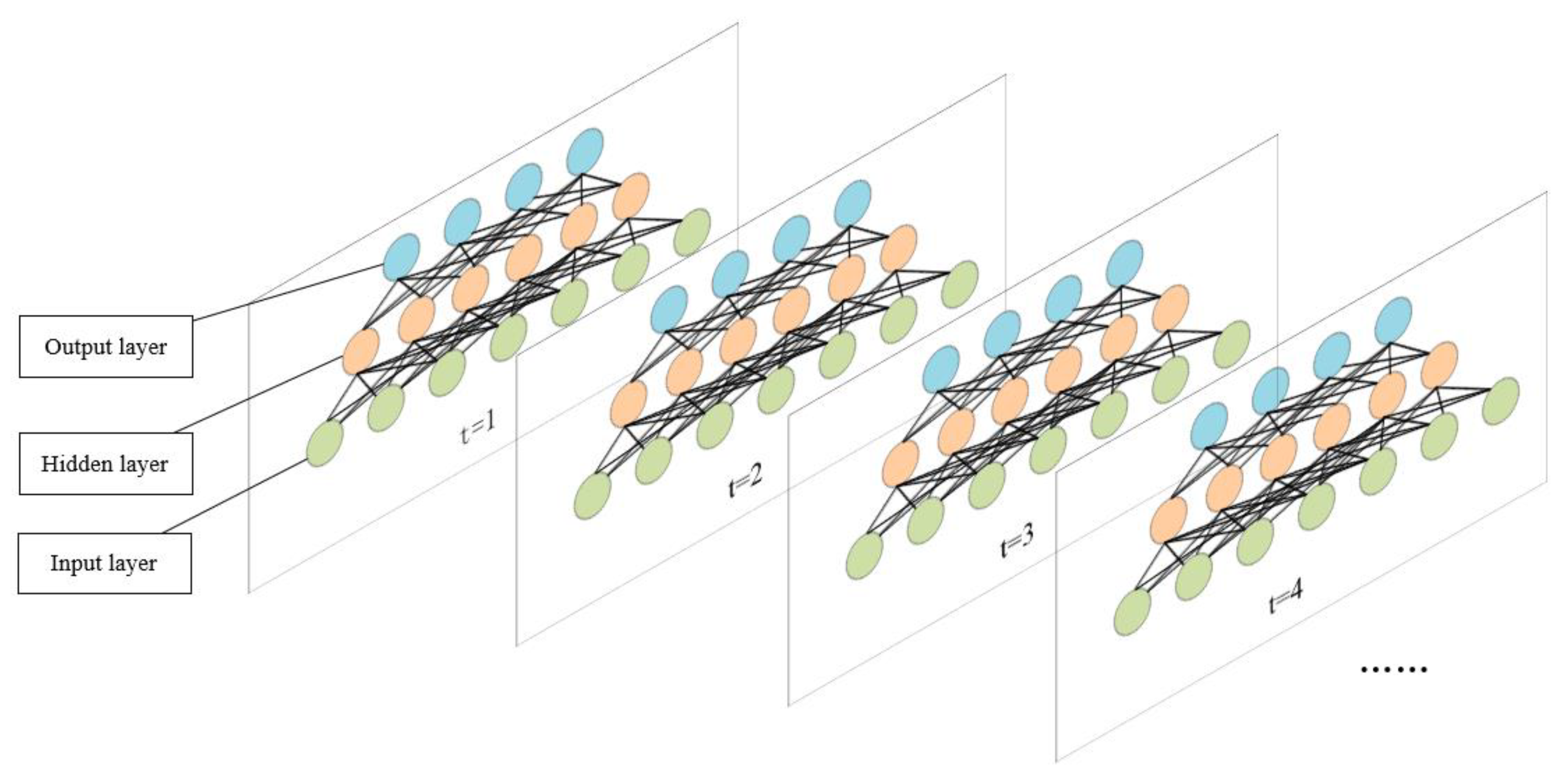
LSTM networks have an outstanding prediction ability for time series and the array signals that are received in the active sonar system are time-series signals. Therefore, we combined an LSTM network with the Kalman filter to effectively improve the prediction ability of the Kalman filtering method in a nonlinear system. We took the filtering process parameters as the inputs of the LSTM network and the model could then output the predicted value that was closest to the real one.
According to reference [24], the state equation and observation equation of the Kalman mathematical model are:
The state update equation of the Kalman filtering method is:
Substituting Formula (4) into Formula (3) can be simplified as:
where, is the prediction state at the time , is the expected prediction state, is the Kalman filter gain, and is the difference between the observed value and the expected prediction state.
The above formulae show that the prediction state of a target at the following time is related to the expected prediction state at the current time, the Kalman gain , and the difference between the observed value and the expected prediction state, which can be expressed as:
Therefore, the inputs of the Kalman filter correction model were the above three factors, the output was the actual state of the moving target , and the inputs and outputs formed a mapping set. The LSTM–NN model could be described as:
Figure 1 shows the schematic diagram of the Kalman filtering method when based on LSTM network correction.
We processed the received data to obtain the position information of the target in unit time. Then, the process parameters of the data that were obtained per second were successively sent to the LSTM network through the Kalman filter. Figure 2 shows this structure.
3. Simulation
We simulated the transmitted and received signals of an active sonar system in the marine environment and established a moving target trajectory diagram, which was based on a two-dimensional plane.
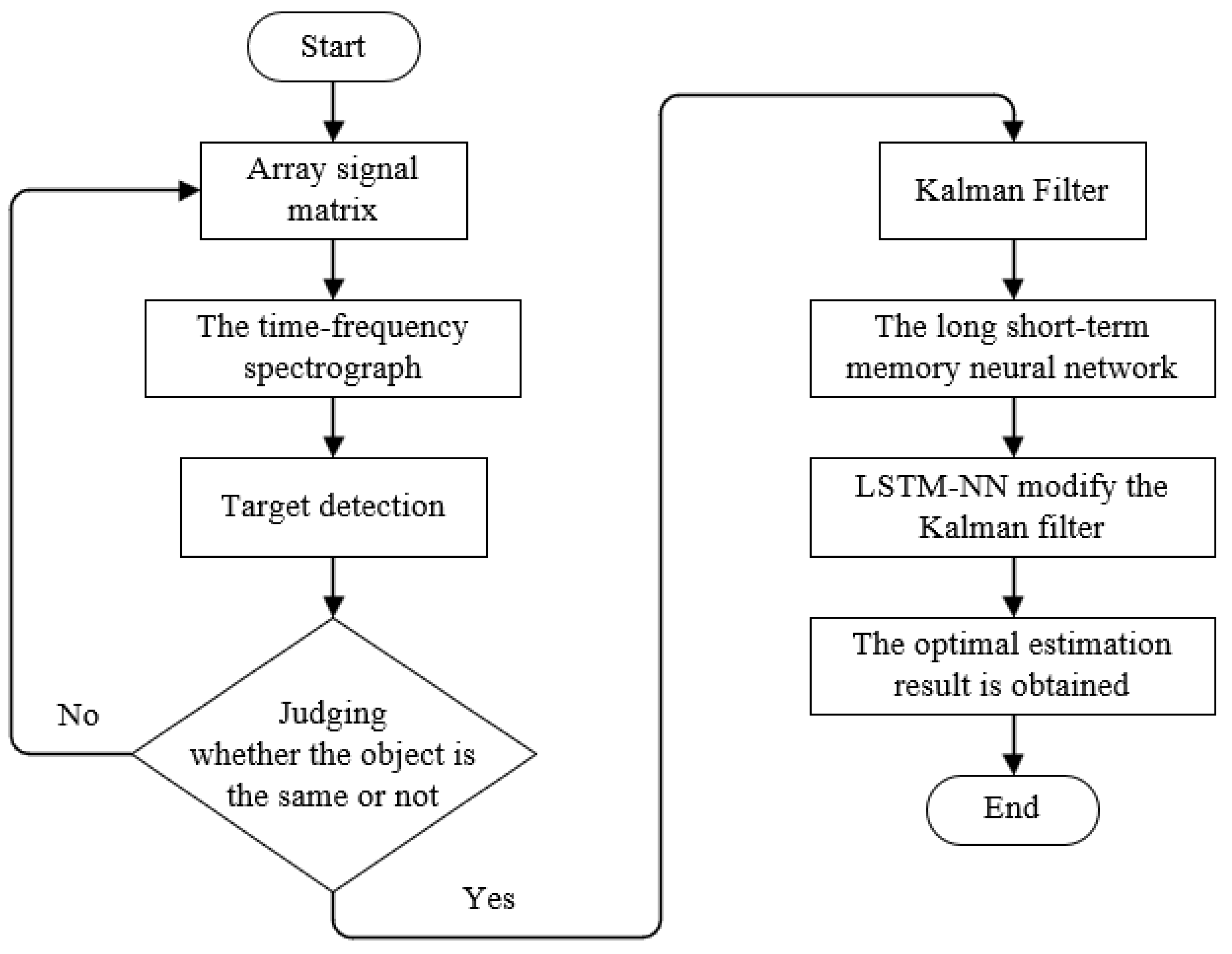
Firstly, the target of the time series was compared using the target detection model to judge whether it was the same target. Secondly, the Kalman filtering method was combined with the LSTM network to obtain the optimal estimation result. Finally, we drew the tracking trajectory of the moving target. Figure 3 shows the simulation flowchart.
3.1. Construction of Array Signals and Generation of Datasets
In this paper, linear frequency modulation (LFM) was used to simulate the transmission signals of the active sonar system. An LFM signal refers to a signal whose frequency changes linearly with time and retains the characteristics of continuous signal and pulse. Using this signal in underwater target tracking can improve the anti-interference ability of active sonar equipment, realize the measurement function of long-distance and residence time resolution, and improve the detection performance of active sonar equipment.
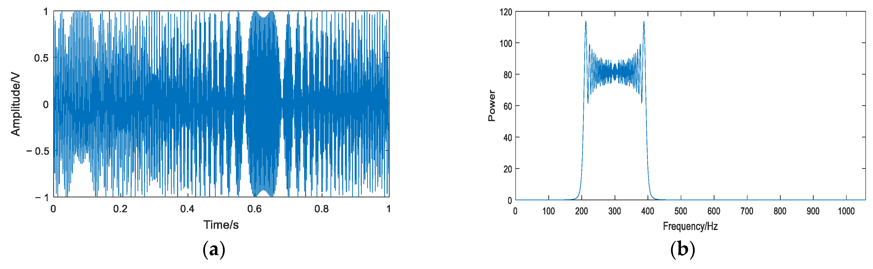
In this experiment, the amplitude of the LFM signal was 1, the starting frequency was 200 Hz, the center frequency was 300 Hz, the sampling frequency was 65 kHz/s, the chirp rate was 200 Hz/s, the sound velocity in water was 1500 m/s, and the transmission duration of the transmitted signal was 1 s. Figure 4 shows the time domain waveform and frequency domain waveform of the transmitted signal. Figure 4a is the time domain waveform of the transmitted signal and Figure 4b is the frequency domain waveform of the transmitted signal.
3.1.1. Generation of Dataset Samples for the Target Detection Model
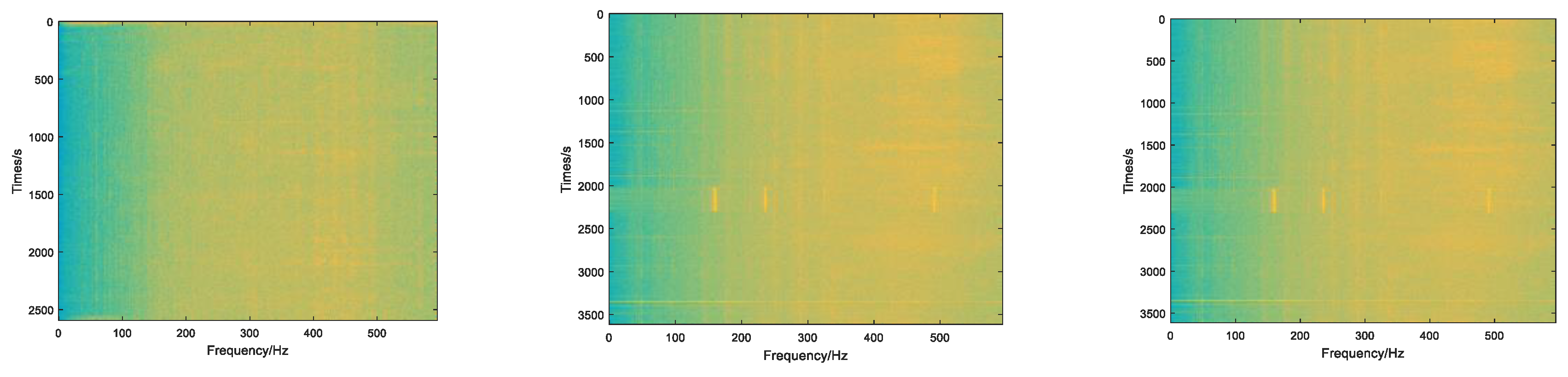
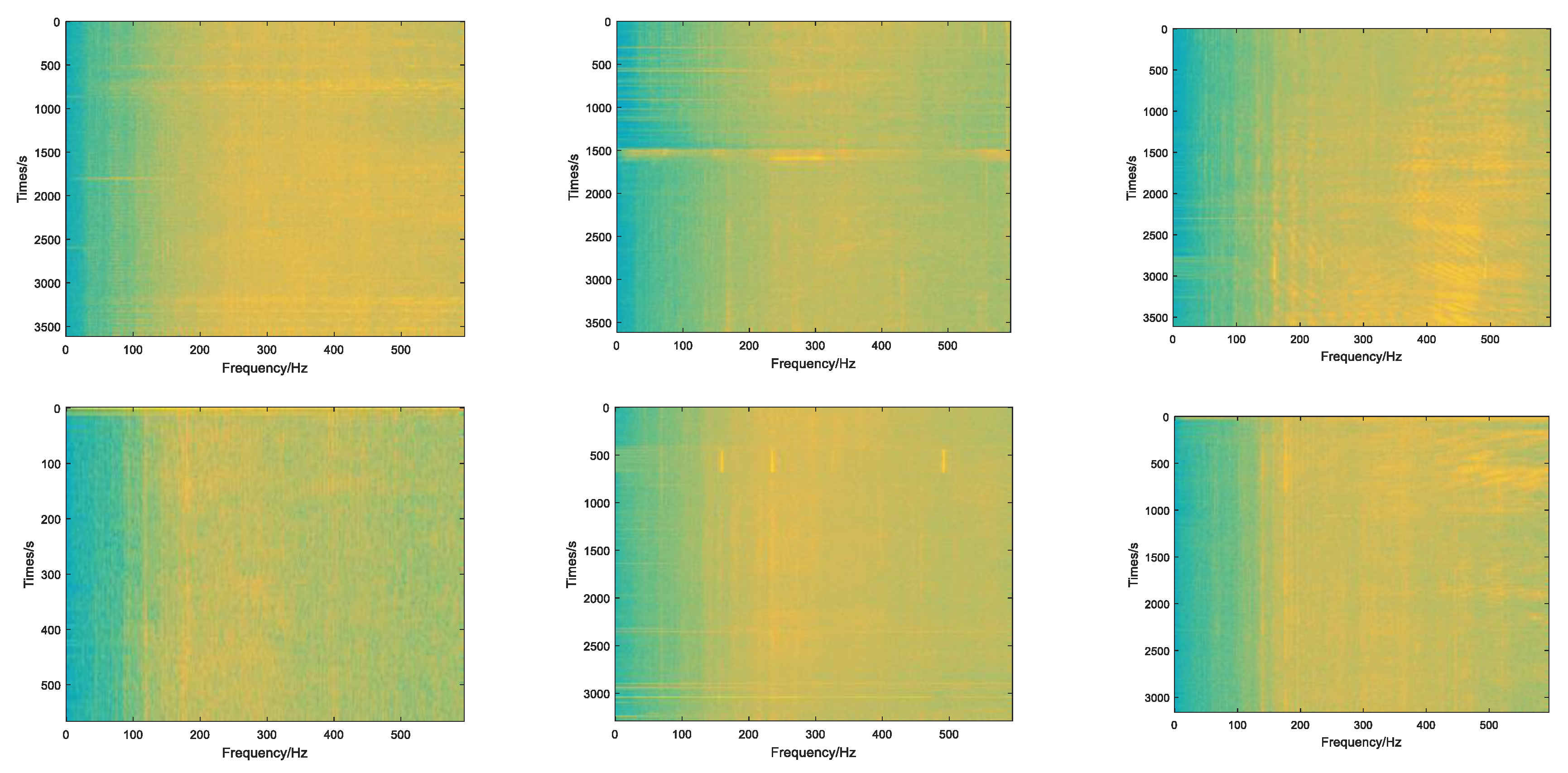
There are both transmitters and receivers in an active sonar system. The transmitter transmits signals continuously. The receiving array element starts to work after the transmitting signal has been transmitted for 1 s to reduce the impact of reverberation and the receiving time lasts for 20 s. The number of receiving array elements was 16 in this experiment, which were arranged as a half-wavelength linear array. At first, we conducted beamforming to enhance the received signal and then the short-term time spectrum could be obtained using the Fourier transform, which was used as the dataset for the target detection model. According to the different characteristics (propeller blade number, shaft frequency, motor noise frequency, signal-to-noise ratio, and target orientation) of targets to be classified, the sample number of each type of target was 2000. We added the background noise of the marine environment as a class of samples and the number of samples was 2000. Assuming that we simulated five types of targets in this experiment, the total number of samples in the final dataset was 12,000. Some of the training samples are shown in Figure 5.
3.1.2. Generation of Dataset Samples for the Target Tracking Model
The five targets in Section 3.1.1 moved along different trajectories. According to the Kalman filtering method, the intermediate calculated values at each time (namely, the expected prediction state at the current time, the Kalman gain , and the difference between the observed value and the expected prediction state) were used as the inputs for the LSTM network and the actual state of the moving target was used as the label output. We simulated the Kalman estimation parameters of the above five types of targets in this experiment. Each type of target had 80 similar samples and the same characteristics. Each sample ran 100 groups of Kalman filtering methods. The total number of samples in the final dataset was 5 × 80 × 100.
3.2. Model Training
3.2.1. Target Detection Model
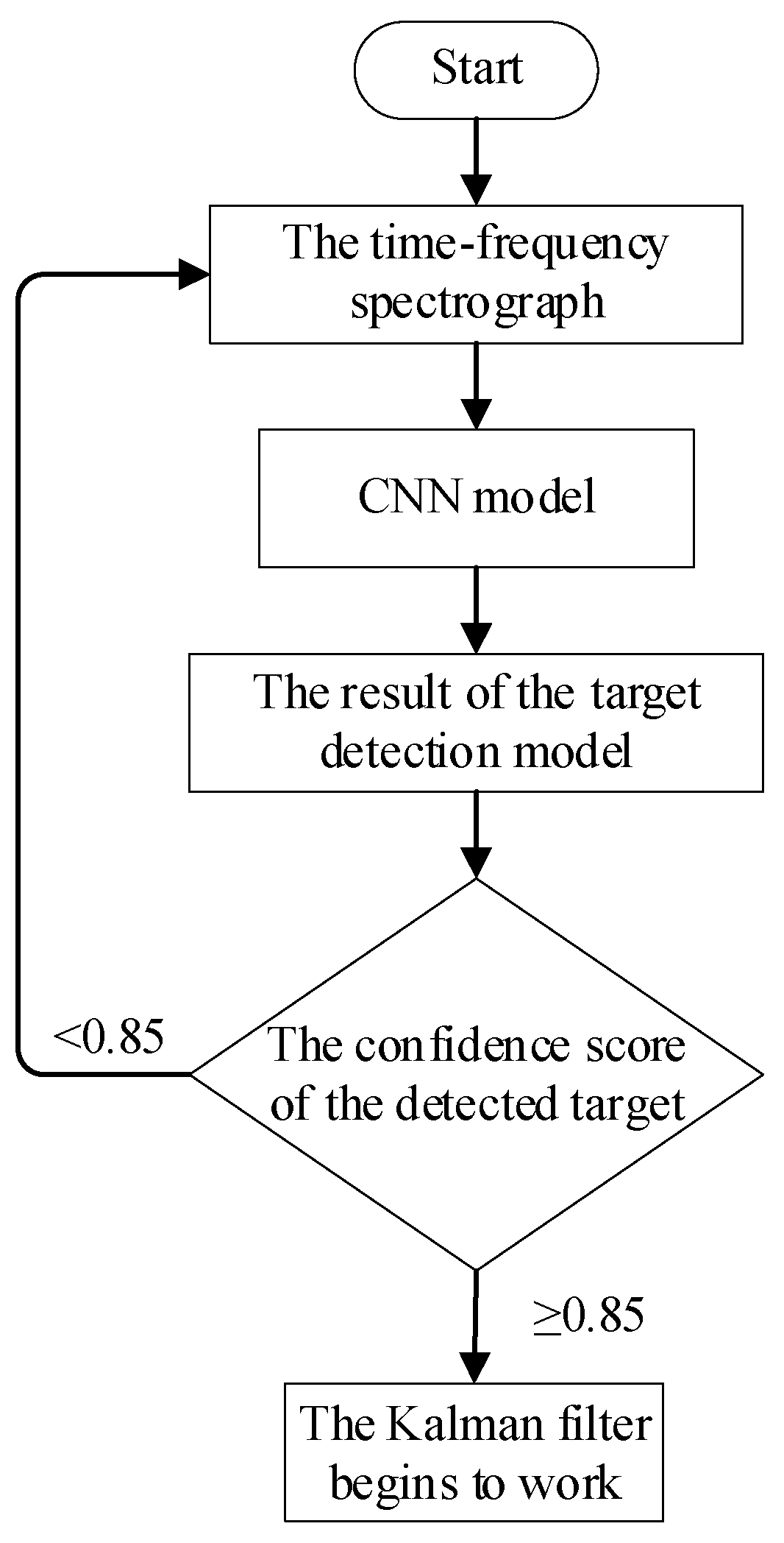
The purpose of the target detection model was to confirm the tracking value of the target to be detected and judge whether to start the target tracking model according to the detection results of the CNN model. We could obtain the type and confidence score of the detected target after the model training. When the confidence score was greater than or equal to 0.85, it was considered that the target had tracking value and the Kalman filter started to work. Figure 6 presents the flowchart of the target detection model.
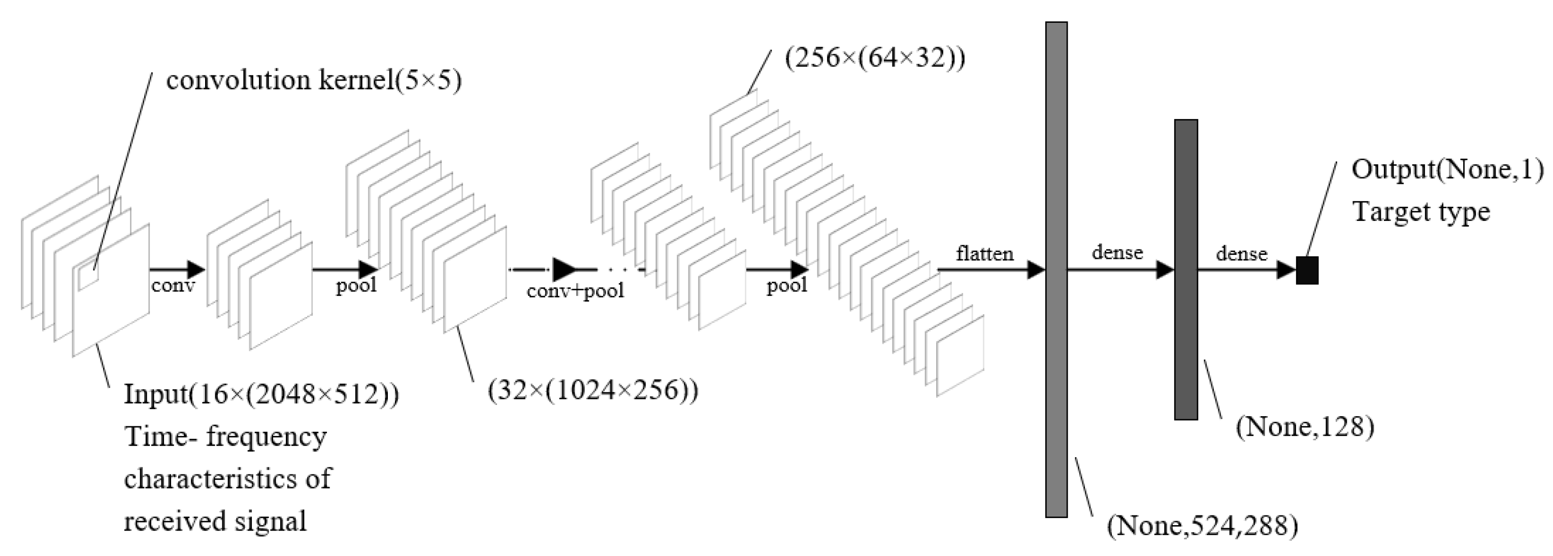
The time–frequency map samples that were obtained in Section 3.1.1 and the corresponding target type were used as of the inputs and output, respectively. The dataset was input into the convolutional neural network (CNN) model for training. By properly adjusting the model parameters, the target recognition accuracy was considerable. When training the model, 70% of the data were used as training samples and 30% were test samples. Figure 7 shows the final model parameters.
The CNN was a five-layer network structure. The activation function used the “ReLU” function, the training optimizer was Adam, the loss function was the multi-classification loss function category “cross-entropy”, and the training batch size was 64.
The accuracy and loss trends of the CNN target detection model after 100 epochs of training are shown in Figure 8.
The training results showed that after 100 epochs, the accuracy rose to 0.998 and the loss approached 0. Therefore, the CNN model could effectively learn the features of the target echo signals using many tests. The accuracy of target detection was sufficient for use in subsequent active underwater acoustic target tracking.
3.2.2. Target Tracking Model
The process parameter dataset of the Kalman filtering method that was obtained in Section 3.1.2 was input into the LSTM network for training and the resulting model after adjusting the model parameters is described below.
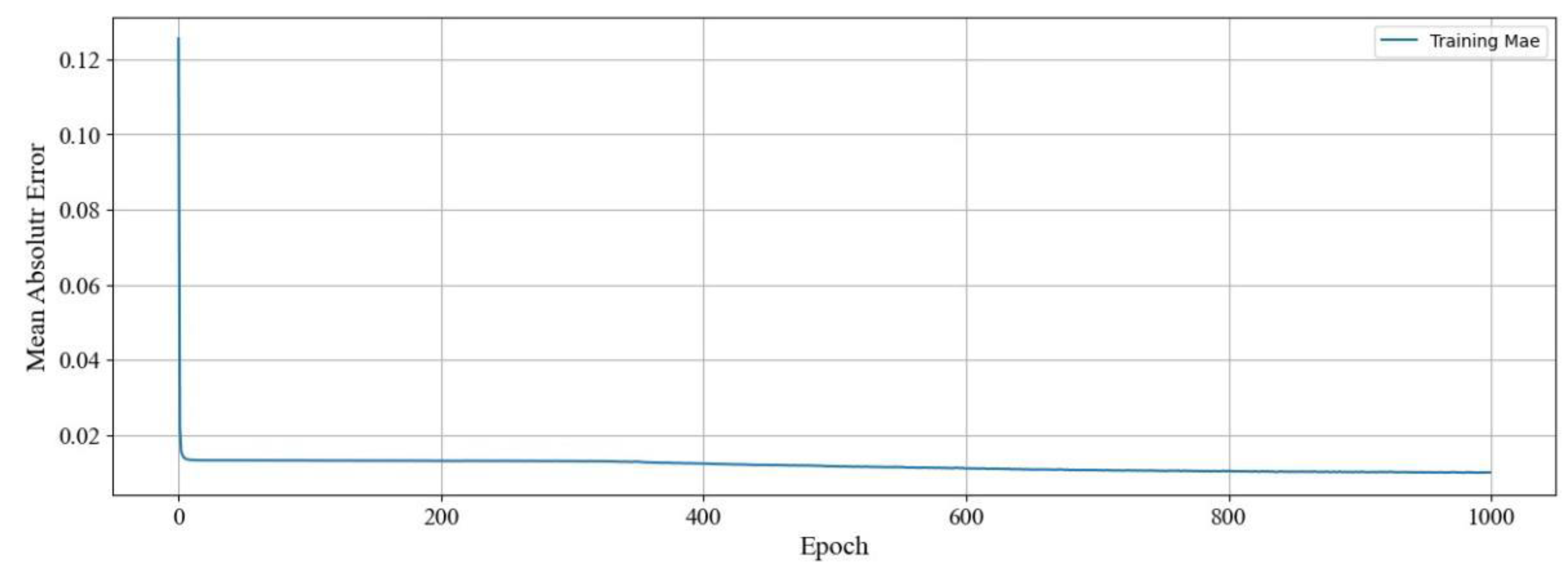
The LSTM network was a three-layer network structure. The hidden layer size was 20 and the hidden layer state had bias. The loss function was the categorical cross-entropy loss function of mean absolute loss (MAE) and the training batch size was 600. The expression for the MAE was as follows:
where is the number of epochs, is the real value, and is the predicted value after neural network training.
The MAE trend of the LSTM network after 1000 epochs of training is shown in Figure 9.
It was concluded from the training results that after 1000 epochs of training, the MAE decreased to 0.01. The batch training test of the model showed that the estimation error of the Kalman filtering method that was based on LSTM network correction, as presented in this paper, was small.
3.2.3. Simulation Results
The established motion trajectory was in the northeast direction and each type of target moved along the same path. We recorded the actual position and the observed distance and orientation information in unit time and transformed them from the polar coordinate system into the Cartesian coordinate system . The initial position information of the target and its velocity in the axis direction were expressed as . We set the initial position of the moving target as , the initial speed as , the process noise variance as , and the observation noise variance as . During the observation scanning period , the total number of samples was 80.
In the simulation experiment, the real path was compared to the tracking results from the Kalman filtering method and the LSTM–Kalman filtering method. Figure 10 shows the final target tracking results.
The above figure shows that the target estimation error of the traditional Kalman filtering method fluctuated with great scope, while the Kalman filter that was corrected by the LSTM network was more in line with the actual result and the prediction error was small. We compared the two trajectories and the results are shown in Figure 11.
Compared to the actual target trajectory, the traditional Kalman filter deviated by less than 50 m, but the fluctuation range was large and the average deviation was 19.58 m. After the Kalman filtering method was corrected using the LSTM model, the deviation was less than 20 m, the average deviation was 7.79 m, and the overall error was reduced by 60%.
4. Experimental Results
To verify the accuracy and stability of our method, we conducted a sea trial in July 2021. We then substituted the obtained sea trial data into the new method for processing and comparative analysis.
The coherent processing interval (CPI) of the system was 0.5 . According to Cramér–Rao theorem, it is obvious that the longer the CPI, the smoother the estimation of the system. However, in this case, considering that the target object was constantly moving, when the selected time was too long, it led to serious inconsistencies between the estimation results and the actual situation. Additionally, the longer the time, the larger the sample size and the required memory and system calculation also surged. Considering the tracking accuracy of the actual system combined with the actual demand and relevant experience, the time interval was set to 0.5 , i.e., 33,280 sampling points.
was the coherent processing interval and the sampling rate of the received signal was 65 , so the sampling points that were obtained in this time period were expressed as:
Assuming that the position in this period of time was a certain value , each sampling point received an estimated value, which was set as . Therefore, within the CPI, the variance was expressed as:
According to the Cramér–Rao theorem:
where is the Fisher information for one data sample.
According to Formula (11), the larger the value, the smaller the Cramér–Rao lower bound, i.e., a more accurate unbiased estimate can be obtained.
However, for the actual system, could not be infinite. Considering the continuous motion of the target to be detected, this paper assumed that the motion state of the target was fixed at 0.5 , i.e., 33,280 sampling points.
The active sonar transmission signal in this test was an LFM signal, with a center frequency of 300 Hz, a sampling frequency of 65 kHz/s, and a bandwidth of 200 Hz. The time domain diagram and frequency domain diagram of the sea trial receiving data (single array element) are shown in Figure 12.
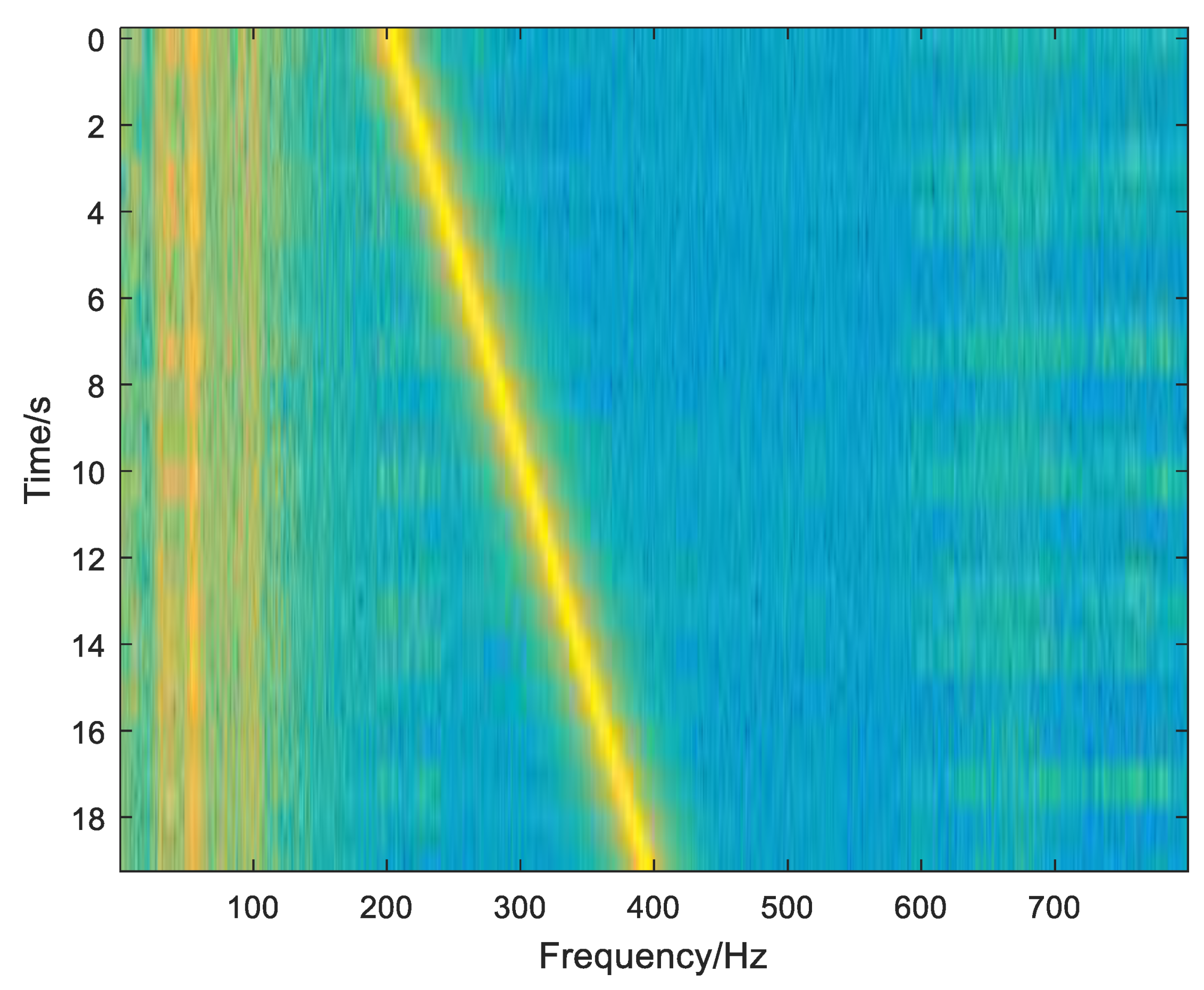
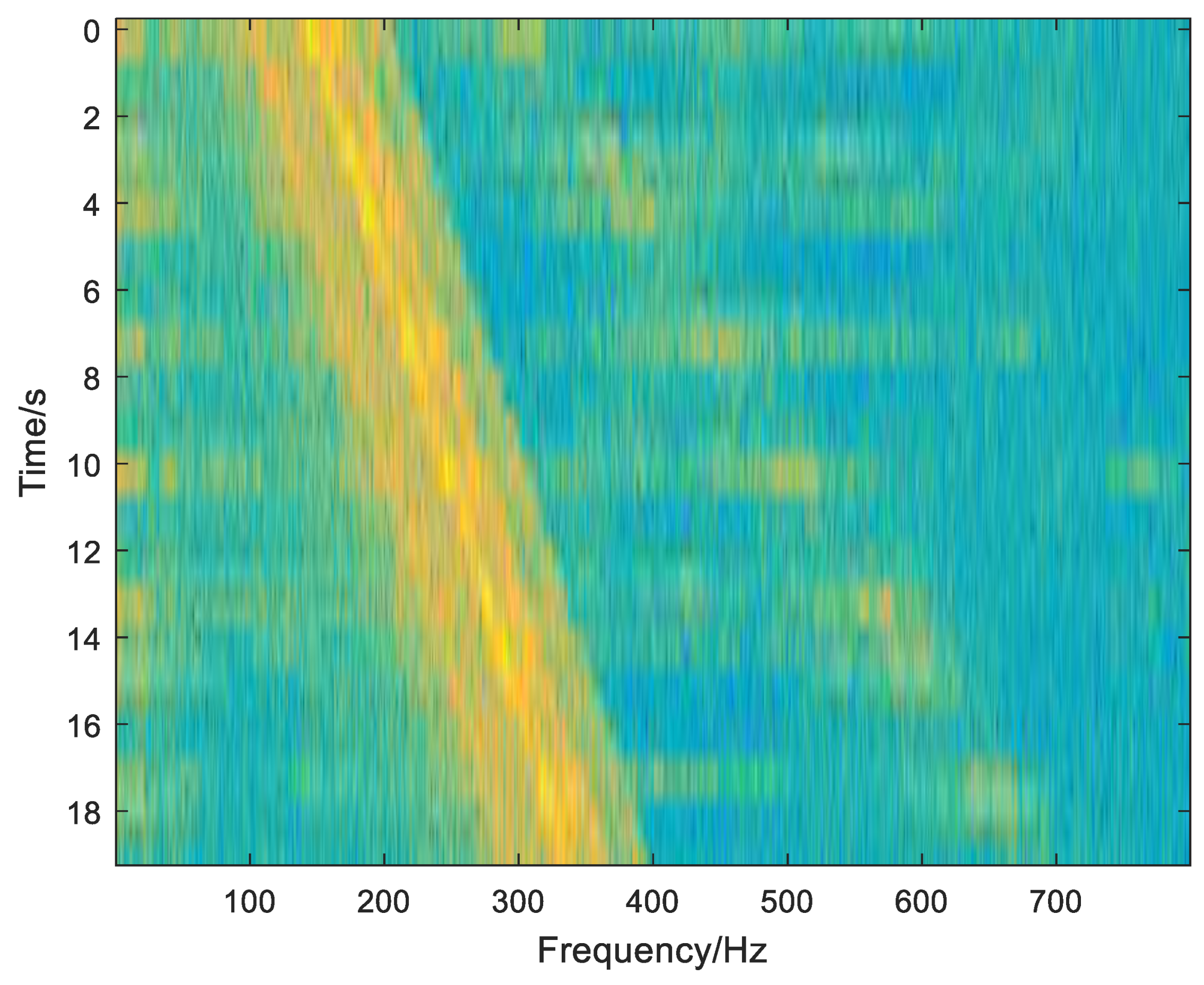
The time spectrum that was analyzed using the short-time Fourier transform was input into the convolutional neural network model for target detection and recognition. Figure 13 and Figure 14 show the corresponding LOFAR diagram and the DEMON diagram.
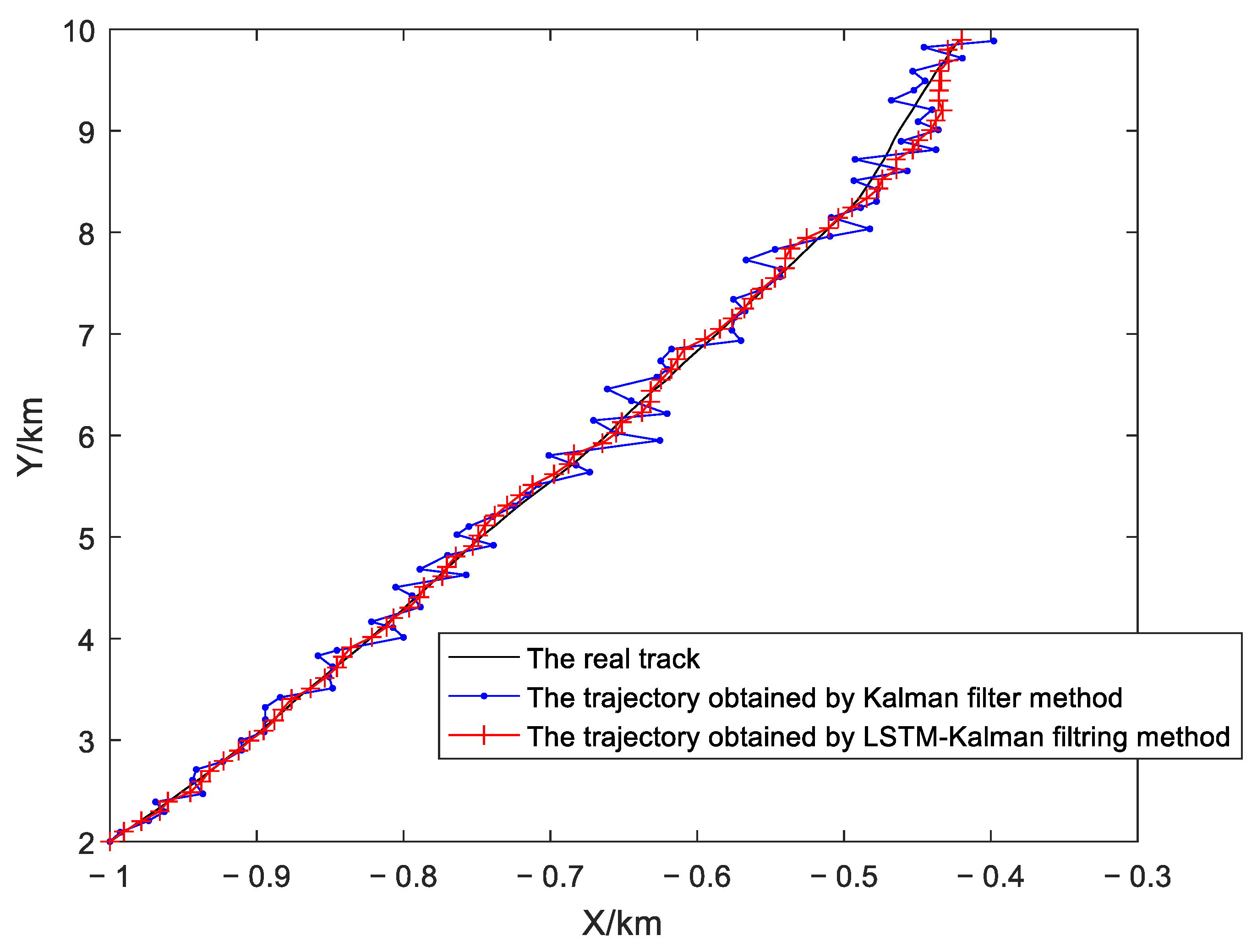
As the underwater target moved nonlinearly, the comparison results of the UKF method and the LSTM–Kalman filtering method, along with the real trajectory, are shown in Figure 15.
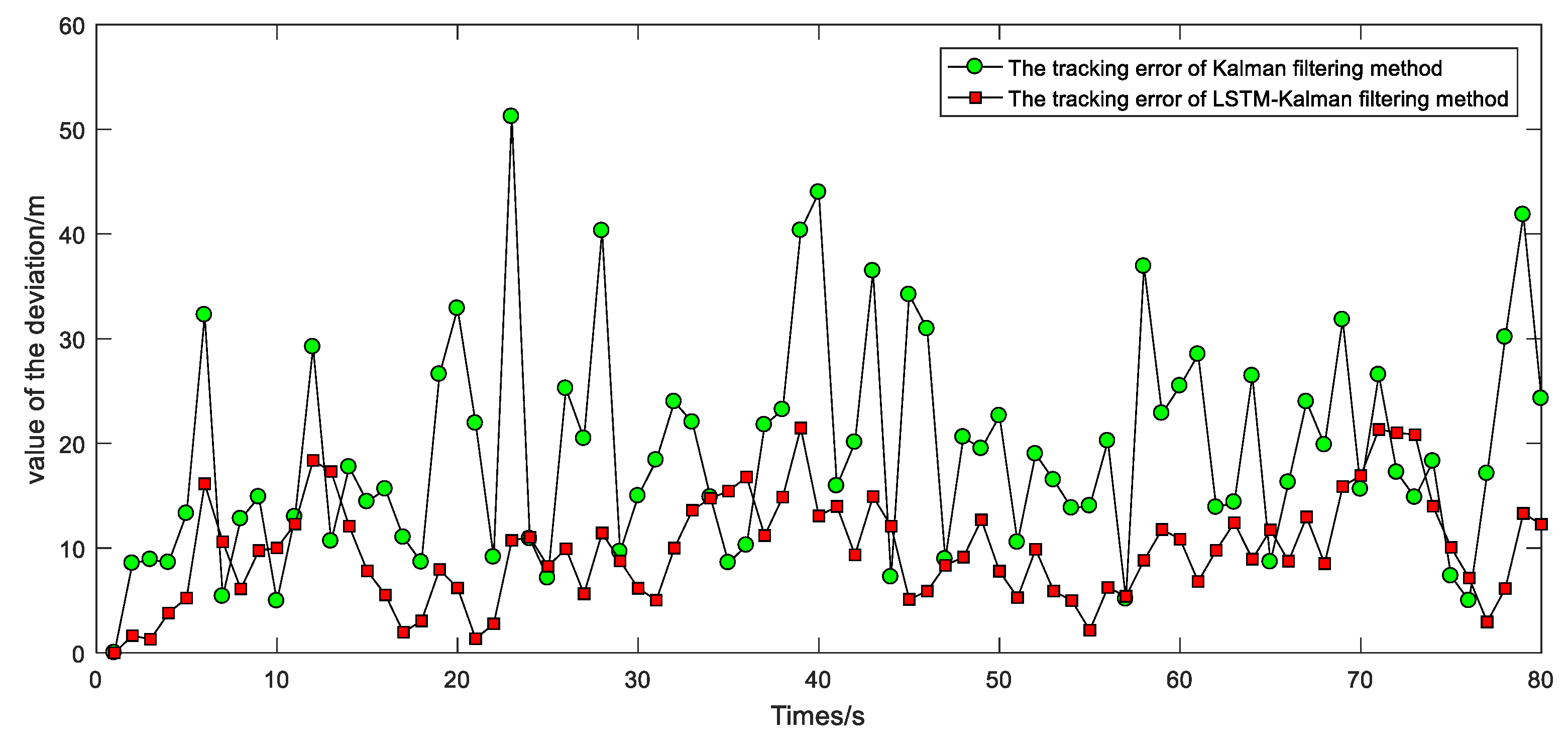
The LSTM–Kalman filtering method was still better than the UKF method in the actual marine environment and fit the actual motion trajectory more closely. The specific error between these two methods is shown in Figure 16.
Compared to the real path, the deviations in the UKF were within 140 m, the average error was 42.45 m, and the variance was 21.08. The results from the LSTM–Kalman filtering method were better, the average error was reduced to 16.94 m, and the variance was 4.79. The relative error of the LSTM–Kalman filtering method was 72.25% lower than that of the UKF method. The results showed that the tracking error of the proposed LSTM–Kalman filtering method was significantly reduced compared to the traditional method and that the new method demonstrated a stable and fast tracking performance.
5. Discussion
Due to the lack of training data, datasets of target signals are not easy to construct and the batch training of labeled data cannot be realized. Therefore, the application of deep learning in the field of target tracking is not widely used. In addition, the traditional Kalman filtering method has high rates of system errors and measurement errors at the last time point. When there is significant interference in the actual situation, it causes large errors in the final estimation results and even the divergence of the filtering results. This impacts target tracking performance, so we proposed a new target tracking method. Firstly, a CNN learned the time–frequency characteristics of a target echo signal, which was conducive to the detection of the subsequent echo signal. Then, an LSTM-NN modified the traditional Kalman filtering method to obtain the optimal estimation result and reduce the impact of accidental errors, such as system errors and observation errors.
We verified the new method using simulation and actual sea experiments. In the simulation experiments, it was found that the closer the trajectory of the moving target to linearity, the more accurate the Kalman filtering method. This also confirmed that a prerequisite of the traditional Kalman filtering method is to assume that the state space model is a linear system. In addition, we used an LSTM network to modify the traditional method, which not only increased the unique time information of the sequence signals and retained the characteristics of the target echo signals that were associated with the time point, but also used the intermediate variables of the traditional Kalman filter for training and learning to extract the core idea of the Kalman filter. Therefore, we combined the two to capitalize on their advantages and ensure their operational efficiency under the conditions of improving the accuracy of the estimation results.
This method avoids the defect of the Kalman filter needing prior knowledge and solves the problem of insufficient training data for target tracking. The LSTM–Kalman filtering method combines the advantages of the two models, uses the framework of the Kalman filter to predict the target motion state in one step, and then uses a neural network to improve the ability of nonlinear relationships. The correction of the traditional Kalman filtering method can be further adjusted to eliminate the estimation deviations that are caused by the inaccuracies of and in practical applications.
Under the experimental conditions described in Section 3, the average error of the Kalman filtering method that was modified using the LSTM network was reduced by 60% compared to the traditional Kalman filter, indicating that its tracking effect was significantly improved. In the actual sea trial described in Section 4, the target tracking environment was more complex and there were many uncertain factors, but the test results were still relatively ideal. Compared to the nonlinear Kalman filtering method, the LSTM–Kalman filtering method reduced the tracking error significantly, showing that the method is suitable for actual marine environments.
6. Conclusions
In this paper, we developed a method for underwater target tracking, which yielded consistently satisfactory results. Firstly, the target echo signal was azimuth weighted using beamforming to enhance the target signal. Then, the beam domain signal was subjected to a short-time Fourier transform to obtain the time–frequency spectrum and the target was detected by the CNN model. Finally, the long-term and short-term memory artificial neural network was modified to the Kalman filtering method to obtain the optimal estimation results. According to the characteristics of the underwater targets, we constructed corresponding datasets and trained the CNN and LSTM-NN models. The test results showed that the model had a high accuracy and could be used for underwater target tracking. Then, we simulated the proposed LSTM–Kalman filtering method and verified it using an actual sea trial. The results showed that this method effectively solved the problem of large deviations in underwater target tracking. It also solved the shortcomings of the traditional Kalman filtering method, which is only suitable for linear systems and requires accurate prior knowledge, and the proposed method also improved the accuracy of the tracking results and the robustness of the system.
On the other hand, considering that targets may become lost or incorrect in the tracking process, a target detection model was added to judge the tracking value at a particular time. When a target appeared for the first time and the confidence score that was output by the target detection model was greater than or equal to 0.85, it indicated that the target was of tracking value and the tracking model started tracking. When a target appeared in the tracking process and the target feature that was detected at the current time was consistent with the target feature of the previous time point, the tracker continued to work, otherwise it started tracking a new target. The method proposed in this paper reduced the amount of calculation required for the system, improved the accuracy of tracking, and significantly reduced the tracking deviations, which has not been achieved using other methods.
The simulation and actual sea trial data indicate that this method is suitable for linear and nonlinear systems, the target position tracking error is significantly reduced compared to the traditional method, and it delivers a stable and fast tracking performance. An innovation of this paper was that an LSTM-NN model was adopted, which made up for the defect of the Kalman filtering method only being suitable for linear systems, reduced the target tracking deviations, and improved the robustness of the system, all of which are important to the practical applications of underwater target tracking. Another innovation was that the target detection model could judge the tracking value of the target and prevent the target from becoming lost or incorrect in the tracking process, which is not available in other methods. The LSTM–Kalman filtering method produced a better tracking performance than the traditional Kalman filtering method and has practical significance for subsequent marine exploration and the establishment of a marine database.
Author Contributions
Conceptualization, C.X. and M.W.; Methodology, C.X. and C.Z.; software, C.X.; validation, C.X., Y.G. and C.Z.; formal analysis, C.Z.; investigation, B.Q.; resources, M.W. and C.X.; data curation, B.Q.; writing—original draft preparation, C.X.; writing—review and editing, C.X., M.W. and C.Z.; visualization, C.X.; supervision, M.W.; project administration, M.W.; funding acquisition, M.W. All authors have read and agreed to the published version of the manuscript.
Funding
This research received no external funding.
Institutional Review Board Statement
Not applicable.
Informed Consent Statement
Not applicable.
Data Availability Statement
The data that support the findings of this study are available from the corresponding author upon reasonable request.
Conflicts of Interest
The authors declare no conflict of interest.
References
- Kumar, D.R. Conditioned measurement fused estimate Unscented Kalman filter for underwater target tracking using acoustic signals captured by Towed array. Appl. Acoust. 2021, 174, 107742. [Google Scholar] [CrossRef]
- Wasiq, A.; Yaan, L.; Kashif, J.; Nauman, A. Performance analysis of gaussian optimal filtering for underwater passive target tracking. Wirel. Pers. Commun. 2020, 115, 61–76. [Google Scholar]
- Yang, Y.L. Comparison of target tracking performance based on Kalman filter and particle filter. J. Jiamusi Univ. (Nat. Sci. Ed.) 2021, 39, 72–75. [Google Scholar]
- Hou, J.; Jing, Z.R.; Yang, Y. Target tracking in standoff jammer using unscented Kalman filter and particle filter with negative information. J. Shanghai Jiaotong Univ. (Sci.) 2014, 19, 181–189. [Google Scholar] [CrossRef]
- Zhang, M.J.; Wan, Y.Y.; Chu, Z.Z. Research on underwater target tracking based on contour detection. Adv. Mater. Res. 2011, 1380, 890–896. [Google Scholar] [CrossRef]
- Kausar, J.; Koteswara Rao, S. Implementation of underwater target tracking techniques for Gaussian and non-Gaussian environments. Comput. Electr. Eng. 2020, 87, 106783. [Google Scholar]
- Rahul, R.K.; Shovan, B.; Nutan, K.T. Continuous-discrete filters for bearings-only underwater target tracking problems. Asian J. Control 2019, 21, 1576–1586. [Google Scholar]
- Liu, B.J.; Ding, M.H.; Zhuang, R. Design of data processing software for underwater multi-target tracking based on line array. Autom. Appl. 2020, 12, 69–71. [Google Scholar]
- Zhang, T.D.; Liu, S.W.; He, X.; Huang, H.; Hao, K.D. Underwater target tracking using forward-looking sonar for autonomous underwater vehicles. Sensors 2019, 20, 102. [Google Scholar] [CrossRef]
- Brandes, T.S.; Dasgupta, N.; Carin, L. Variational Bayesian particle filtering for underwater target localization and tracking. J. Acoust. Soc. Am. 2009, 125, 2578. [Google Scholar] [CrossRef]
- Li, Z.; Li, Y.; Huang, Y.; Hhuang, H.N. Study of automatic continuous tracking and location algorithm for underwater target. J. Instrum. 2012, 33, 520–528. [Google Scholar]
- Omkar, L.J.; S.Koteswara, R.; Kausar, J. Unscented particle filter approach for underwater target tracking. Int. J. E-Collab. 2021, 17, 29–40. [Google Scholar]
- Kumar, D.V.A.N.R. Hybrid unscented Kalman filter with rare features for underwater target tracking using passive sonar measurements. Optik 2021, 226, 165813. [Google Scholar] [CrossRef]
- Lamyae, F.; Siham, B.; Hicham, M. Mathematical model and attitude estimation using extended colored Kalman filter for transmission lines inspection’s unmanned aerial vehicle. IIETA 2021, 54, 529–537. [Google Scholar]
- Zhao, M.; He, S.Q.; Shi, C.; Jiang, W.J. A Kalman filter indoor positioning method based on neural network correction parameters. Mod. Electron. Technol. 2020, 43, 21–24. [Google Scholar]
- Donghyun, L.; Minkyu, L.; Hosung, P.; Kang, Y.; Jeong-Sik, P.; Gil-Jin, J.; Ji-Hwan, K. Long short-term memory recurrent neural network-based acoustic model using connectionist temporal classification on a large-scale training corpus. China Commun. 2017, 14, 23–31. [Google Scholar]
- Levent, I.; Bulent, S.; Erhan, S.; Huseyin, I. An evolutionary computing approach for the target motion analysis (TMA) problem for underwater tracks. Expert Syst. Appl. 2008, 36, 3866–3879. [Google Scholar]
- Xia, Y.L. Review on the development of cyclic neural networks. Comput. Knowl. Technol. 2019, 15, 182–184. [Google Scholar]
- Yu, Y.; Si, X.; Hu, C.H.; Zhang, J.X. A review of recurrent neural networks: LSTM cells and network architectures. Neural Comput. 2019, 31, 1235–1270. [Google Scholar] [CrossRef]
- Zhao, J.H.; Gao, H.B.; Liu, Y.C.; Cheng, B. Speech recognition algorithm based on neural network and hidden Markov model. J. China Univ. Posts Telecommun. 2018, 25, 28–37. [Google Scholar]
- Alex, S. Fundamentals of recurrent neural network (RNN) and long short-term memory (LSTM) network. Phys. D Nonlinear Phenom. 2020, 404, 132306. [Google Scholar]
- Bertinetto, L.; Valmadre, J.; Henriques, J.F.; Vedaldi, A.; Torr, P.H.S. Fully-convolutional siamese networks for object tracking. Eur. Conf. Comput. Vis. 2016, 9914, 850–865. [Google Scholar]
- Shi, L.; Xu, J.L. Two-branch object tracking algorithm based on siamese network. Softw. Guide 2021, 20, 214–218. [Google Scholar]
- Huang, X.P.; Wang, Y.; Miu, P.C. Principle and Application of Target Location and Tracking—MATLAB Simulation, 1st ed.; Electronic Industry Press: Beijing, China, 2018; pp. 76–78. [Google Scholar]
Figure 1.
The schematic diagram of the LSTM–Kalman filtering method.

Figure 2.
The internal structure of the LSTM-NN.

Figure 3.
The simulation flowchart of the LSTM–Kalman filtering method.

Figure 4.
The time domain waveform and frequency domain waveform of the transmitted signal: (a) the time domain waveform of the transmitted signal; (b) the frequency domain waveform of the transmitted signal.
Figure 4.
The time domain waveform and frequency domain waveform of the transmitted signal: (a) the time domain waveform of the transmitted signal; (b) the frequency domain waveform of the transmitted signal.

Figure 5.
Partial training set of samples for the target detection model.


Figure 6.
The flowchart of the target detection model.

Figure 7.
Network structure of the target detection model.

Figure 8.
Accuracy and loss of the CNN model after 100 epochs of training: (a) the accuracy of the CNN model after 100 epochs of training; (b) the loss of the CNN model after 100 epochs of training.
Figure 8.
Accuracy and loss of the CNN model after 100 epochs of training: (a) the accuracy of the CNN model after 100 epochs of training; (b) the loss of the CNN model after 100 epochs of training.

Figure 9.
MAE of the LSTM-NN model after 1000 epochs of training.

Figure 10.
Comparison of the real path, the tracking trajectory that was obtained using the Kalman filtering method, and the tracking trajectory that was obtained using the LSTM–Kalman filtering method.
Figure 10.
Comparison of the real path, the tracking trajectory that was obtained using the Kalman filtering method, and the tracking trajectory that was obtained using the LSTM–Kalman filtering method.

Figure 11.
Comparison diagram of the target tracking deviations between the Kalman filtering method and the LSTM–Kalman filtering method.
Figure 11.
Comparison diagram of the target tracking deviations between the Kalman filtering method and the LSTM–Kalman filtering method.

Figure 12.
The time domain diagram and frequency domain diagram of the receiving data: (a) the time domain diagram of the receiving data; (b) the frequency domain diagram of the receiving data.
Figure 12.
The time domain diagram and frequency domain diagram of the receiving data: (a) the time domain diagram of the receiving data; (b) the frequency domain diagram of the receiving data.

Figure 13.
LOFAR diagram of the receiving data.

Figure 14.
DEMON diagram of the receiving data.

Figure 15.
Comparison of the real trajectory, the tracking trajectory that was obtained using the Kalman filtering method, and the tracking trajectory that was obtained using the LSTM–Kalman filtering method.
Figure 15.
Comparison of the real trajectory, the tracking trajectory that was obtained using the Kalman filtering method, and the tracking trajectory that was obtained using the LSTM–Kalman filtering method.

Figure 16.
Comparison diagram of the target tracking deviations between the Kalman filtering method and the LSTM–Kalman filtering method.
Figure 16.
Comparison diagram of the target tracking deviations between the Kalman filtering method and the LSTM–Kalman filtering method.

Publisher’s Note: MDPI stays neutral with regard to jurisdictional claims in published maps and institutional affiliations. |
© 2022 by the authors. Licensee MDPI, Basel, Switzerland. This article is an open access article distributed under the terms and conditions of the Creative Commons Attribution (CC BY) license (https://creativecommons.org/licenses/by/4.0/).
Share and Cite
MDPI and ACS Style
Wang, M.; Xu, C.; Zhou, C.; Gong, Y.; Qiu, B. Study on Underwater Target Tracking Technology Based on an LSTM–Kalman Filtering Method. Appl. Sci. 2022, 12, 5233. https://0-doi-org.brum.beds.ac.uk/10.3390/app12105233
AMA Style
Wang M, Xu C, Zhou C, Gong Y, Qiu B. Study on Underwater Target Tracking Technology Based on an LSTM–Kalman Filtering Method. Applied Sciences. 2022; 12(10):5233. https://0-doi-org.brum.beds.ac.uk/10.3390/app12105233
Chicago/Turabian StyleWang, Maofa, Chuzhen Xu, Chuanping Zhou, Youping Gong, and Baochun Qiu. 2022. "Study on Underwater Target Tracking Technology Based on an LSTM–Kalman Filtering Method" Applied Sciences 12, no. 10: 5233. https://0-doi-org.brum.beds.ac.uk/10.3390/app12105233
Note that from the first issue of 2016, this journal uses article numbers instead of page numbers. See further details here.