
Low-Light Image Enhancement Method Based on Retinex Theory by Improving Illumination Map


1
College of Computer and Information, Hohai University, Nanjing 211100, China
2
School of Artificial Intelligence, Nanjing University of Information Science and Technology, Nanjing 210044, China
3
School of Engineering, Shantou University, Shantou 515063, China
*
Author to whom correspondence should be addressed.
Appl. Sci. 2022, 12(10), 5257; https://0-doi-org.brum.beds.ac.uk/10.3390/app12105257
Submission received: 19 April 2022
/
Revised: 19 May 2022
/
Accepted: 20 May 2022
/
Published: 23 May 2022
Abstract
:Recently, low-light image enhancement has attracted much attention. However, some problems still exist. For instance, sometimes dark regions are not fully improved, but bright regions near the light source or auxiliary light source are overexposed. To address these problems, a retinex based method that strengthens the illumination map is proposed, which utilizes a brightness enhancement function (BEF) that is a weighted sum of the Sigmoid function cascading by Gamma correction (GC) and Sine function, and an improved adaptive contrast enhancement (IACE) to enhance the estimated illumination map through multi-scale fusion. Specifically, firstly, the illumination map is obtained according to retinex theory via the weighted sum method, which considers neighborhood information. Then, the Gaussian Laplacian pyramid is used to fuse two input images that are derived by BEF and IACE, so that it can improve brightness and contrast of the illuminance component acquired above. Finally, the adjusted illuminance map is multiplied by the reflection map to obtain the enhanced image according to the retinex theory. Extensive experiments show that our method has better results in subjective vision and quantitative index evaluation compared with other state-of-the-art methods.
1. Introduction
With the rapid development of modern computer and multimedia information technology, digital image processing systems have been widely used in industrial production [1], scientific research [2], intelligent transportation [3], and other fields. However, the process of image acquisition is complex and affected by many factors, resulting in various image defects. Insufficient lighting conditions, such as indoor, cloudy, or night conditions, often lead to a serious decline in image quality [4].
Researchers have pursued various improvements from both the hardware and software perspectives. The former is the development of image acquisition equipment [5,6], such as using professional low light level cameras (e.g., Sony, SiOnyx, and Photonis), but they are expensive and not suitable for daily life. The latter is to improve the collected image through digital image processing. The main research direction of this paper was software-based low-light image enhancement.
Enhancing the visual quality of images captured under weak light conditions is a difficult problem. These images usually appear with low contrast, low resolution, high noise, and over-exposure, due to insufficient light and gain, which affect our visual effects seriously. Consequently, low-light image enhancement technology, which aims to improve the overall brightness, local contrast, and detail information of raw images, has been widely studied [7,8,9,10].
Directly increasing the image brightness is the most intuitive and simplest method. Typical algorithms use histogram equalization (HE) and grayscale transformation, which enhance pixel values through mathematical functions. HE and its derivative algorithms [11,12,13,14,15] are widely used due to their simplicity and effectiveness. Grayscale transformation uses a mathematical function to change grayscale values, and gamma correction (GC) is one of the most widely used methods [16,17,18]. These methods enhance the entire image to the same degree regardless of whether the area is dark or not, which easily causes overexposure. Retinex theory [19,20,21,22,23,24,25] assumes that an image can be decomposed into an illumination component and a reflection component, and the latter is used as the final enhanced image. Single-scale retinex (SSR) [20], multi-scale retinex (MSR) [21], and multi-scale retinex with color restoration (MSRCR) [22] are typical algorithms based on retinex theory. However, these methods enhance the image by eliminating illumination, resulting in loss of information.
Image fusion-based enhancement algorithms have attracted the attention of scholars because they do not require any physical model but only fuse useful information from multiple images [26,27,28,29]. Fu et al. [27] introduced a fusion method based on a variety of mature image proposing technologies to improve image quality (MF). Unlike the classical retinex method, this method improves shimmering images by maintaining and enhancing image illumination. However, for the enhancement of image brightness, an inverse tangent function is still used, and the enhancement degree of global brightness is the same, leading to a certain degree of overexposure. Dai et al. [28] proposed a fractional-order mask and the fusion framework model (FFM) for low-light image enhancement. However, the model produces an overall darker and less visually appealing result.
Recently, deep learning-based methods have been proposed, which extract numerous image features from datasets and hence can effectively improve image quality [30,31,32,33]. Ren et al. [30] proposed a trainable hybrid network that consists of two distinct streams to obtain a clear image. Park et al. [32] present a dual autoencoder network model to enhance low-light images and reduce noise by combining the stacked and convolutional autoencoders. Chen et al. [33] designed a so-called Retinex-Net (Ret-Net) network, which includes a decom-net for decomposition and an enhancement-net for illumination adjustment. However, these algorithms rely on many natural images for training the network, heavily depend on the number of input images and are computationally complex and time-consuming.
Although many researchers have proposed numerous low-light image enhancement algorithms, several problems still need to be addressed. For instance, some methods may not be able to completely extract contents at very dark regions, some may pose the risk of excessive enhancement, and some may blur detail information.
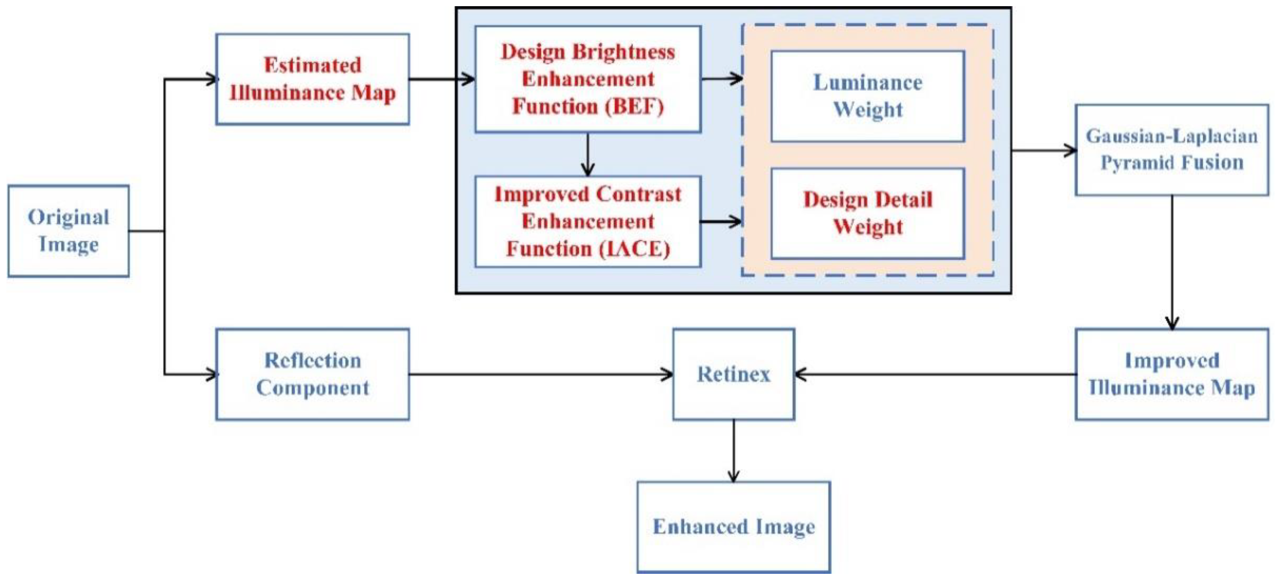
In this paper, we propose a retinex theory-based algorithm to enhance images well and solve the above problems. The proposed method enhances the bright and dark areas to varying degrees and comprises three parts: (1) estimation of illumination component and reflection component from raw image; (2) blending two input images obtained by BEF and IACE to enhance the illumination component by Gaussian Laplacian pyramid; and (3) deriving the final enhanced image based on retinex theory. The general process of the proposed model is shown in Figure 1, and the main innovations are marked in red font and explained in detail in Section 3.2.
Our main contributions can be summarized as follows.
- (1)
- We designed a neighborhood-weighted illuminance map estimation algorithm by considering the correlation among pixels. The estimated illuminance map carries important information about objects’ structure in the visual scene.
- (2)
- We designed two functions to acquire input images for fusion, including a brightness enhancement function (BEF) and an improved adaptive contrast enhancement (IACE). The BEF can not only highlight the contents within dark areas but also retain the details within bright areas, and the IACE can enhance contrast while avoiding noise amplification.
- (3)
- We found that significant details exist in regions with large gradients, and large variances are rich in information. Hence, we designed a detail weight for the fusion procedure by considering the gradient and variance of local regions.
- (4)
- Compared with previous algorithms, the proposed method has several advantages. Firstly, the brightness of the illumination map is differentially enhanced (i.e., the light and dark areas of the image are enhanced to different degrees), so that not only is the content of the dark areas displayed, but also the details of the bright areas are not blurred. Then, the high-frequency component in contrast enhancement tends to amplify the noise, and in this paper, the image is enhanced in the form of a piecewise function to reduce noise. Finally, the weight based on gradient and variance enriches the image details.
The rest of this paper is organized as follows. Section 2 discusses the relevant work. The proposed method is detailed in Section 3. The performance of the proposed method is evaluated both quantitatively and qualitatively in Section 4. Section 5 highlights some limitations of the proposed work and future research directions. Section 6 concludes the paper.
2. Related Works
In this section, we focus on reviewing and analyzing some basic contents required for the proposed model. Specifically, we first introduce the retinex theory, then give the formula and corresponding curve graphs used in the two fused images, and finally explain the importance of gradient and variance for designing the weight in the subsequent work.
2.1. Retinex Theory
Retinex theory [19] divides an image into a reflection component and an illumination component:
where , and are original image and reflection image and illumination image, respectively; and denotes three color channels of RGB (red, green, blue). The algorithm based on retinex theory aims to enhance the illuminance component to improve the quality of low-light images [27].
2.2. Gamma Correction, Sigmoid Function and Sine Function
GC and sigmoid function are classical methods to enhance image brightness. The formula for GC is
where is the enhanced image and is a constant. The current and subsequent are normalized images taking values between [0, 1]. sigmoid function hardly changes outside the interval [−10, 10], but the pixel values of the images are all greater than 0. Therefore, we intercept the definition domain of the sigmoid function between [0, 10] and adjust the formula accordingly, the final formula is shown below:
In order to significantly improve the brightness of the image, we need to intercept the part of the sigmoid function within [0, 1] and further normalize it. Hence, the specific formula becomes:
2.3. Correlation Study of Gradient and Variance
The gradient of an image measures the change rate of pixels in the horizontal and vertical directions and is commonly used to provide more detailed information for edge detection and reconstruction [34,35,36,37,38,39]. The variance reflects the high-frequency component. The larger the variance, the better the visual effect is, and the easier different objects are to distinguish.
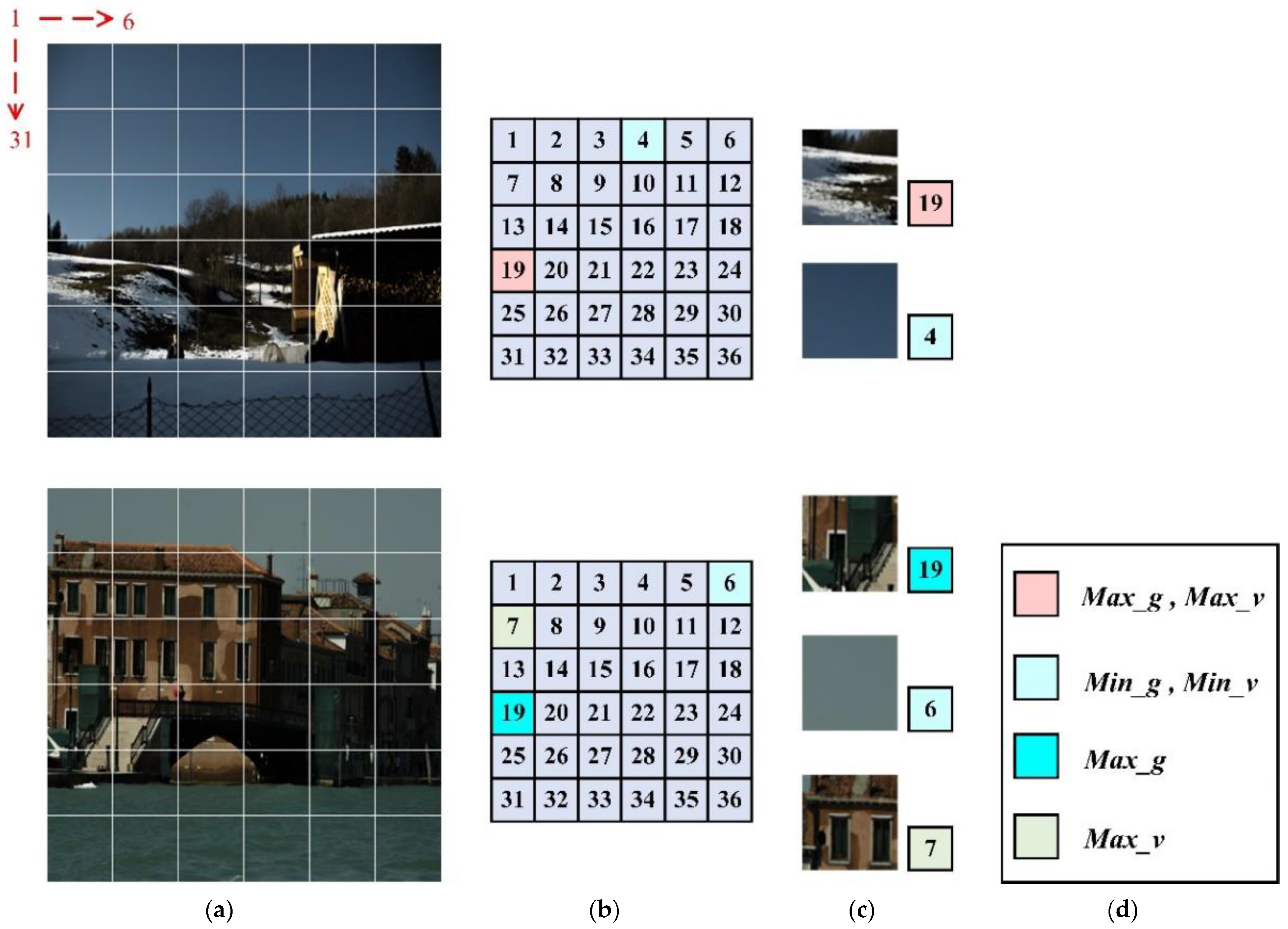
Figure 2 shows two images, either of which is divided into 36 small regions of the same size. The number in Figure 2b is the corresponding number of each region. Figure 2c illustrates the regions with the maximum gradient () and the minimum gradient () and the maximum () and minimum variance (). From Figure 2, it can be seen that the regions with and contain rich information, while the regions with and only have plain contents. So, the regions with and are vital for detail processing.
3. The Proposed Algorithm
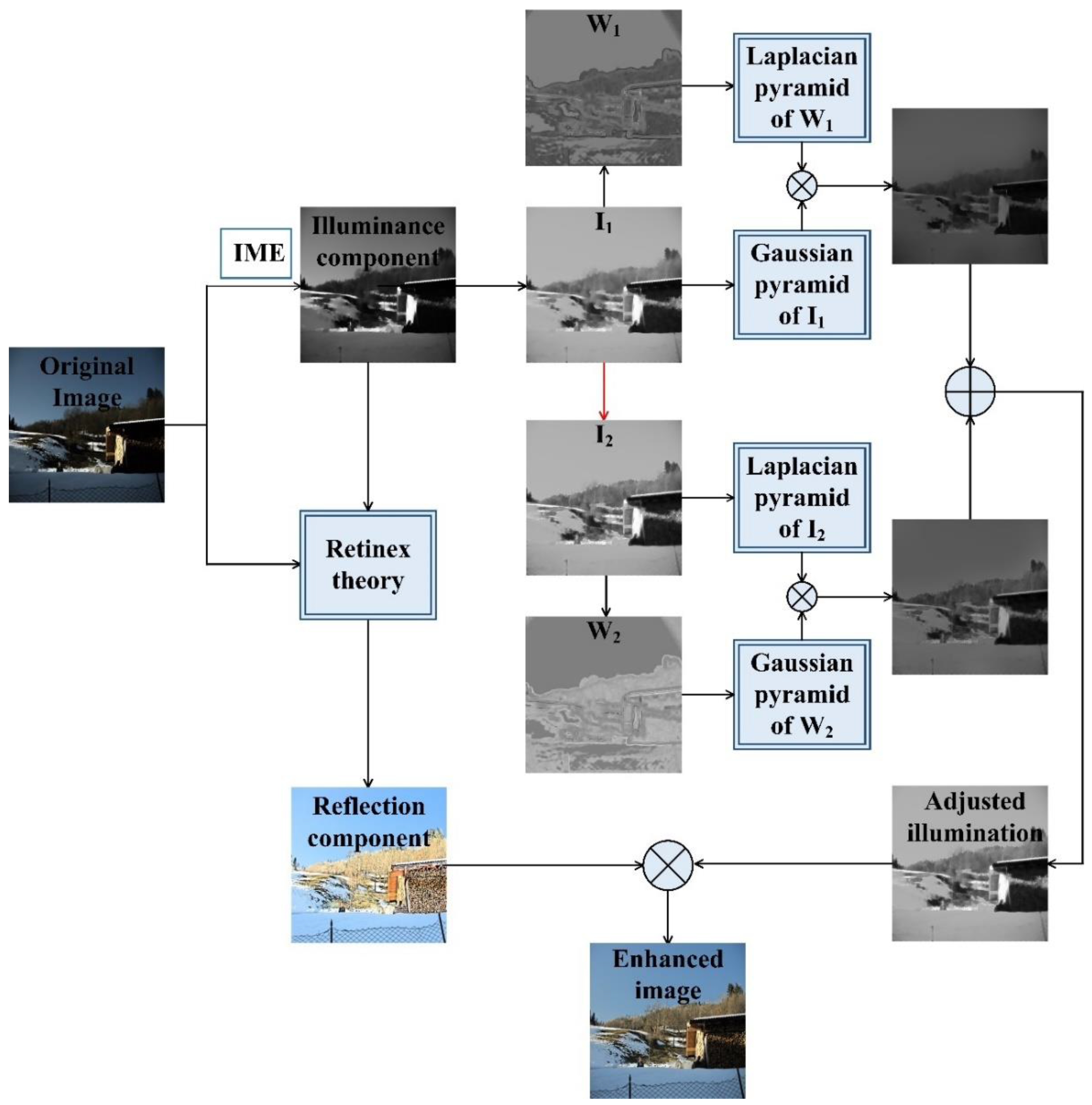
The objective of the proposed method is the enhancement of a low-light image by enhancing the brightness and contrast of the illuminance map. Firstly, a neighborhood-based approach is proposed to estimate the illuminance component, and then obtain the reflection component through the retinex theory. Secondly, differential enhancement is applied to each region in the illuminance component, that is, the luminance is substantially increased in darker regions and hardly enhanced in brighter regions. Contrast enhancement uses the form of piecewise function to update the image pixel by pixel to reduce noise. Then, the two enhanced images are used to obtain the adjusted illumination map using the Gaussian–Laplacian pyramid fusion algorithm. Finally, the improved illumination map is multiplied by the reflection component to obtain the final enhancement result. Figure 3 shows the flowchart of the algorithm in this paper. As follows, we introduce our method in this section with all necessary details.
3.1. Estimation of Illumination Component and Reflection Component
In this section, an illuminance map estimation (IME) algorithm is proposed based on the neighborhood information of pixels. Specifically, the pixel’s value is updated using a weighted sum with the neighboring pixels, followed by the morphological closure algorithm and guided filter for refinement. The specific steps are as follows.
Let be the i-th pixel’s neighborhood, the maximum value of R, G, and B at the position , j the pixel’s position inside , the weight value of position j. The neighborhood-based illuminance map is derived from:
Considering the fact that the greater the difference among pixel values, the lower the weight that should be constructed, or conversely, the greater the weight value at the position , the smaller the difference between and is, we designed the following weight:
where is the maximum weight in the neighborhood. We normalize the weights to obtain the final . The above idea is similar to the inverse distance weight (IDW) method [40,41,42].
Then, we use the morphological closure algorithm [27,43] and Guided filter [44] to refine the illumination map. The neighborhood-based illuminance map from Equation (5) is preliminarily refined by:
where denotes the structuring element and is the closing operation. Dividing by 255 is used to map the range to [0, 1] for the downstream operations. The final refined illumination map is obtained by:
where is the value component of the guidance image in HSV space and is the filter kernel:
Here is the window centered at the i-th pixel and is the number of pixels within ; and are the mean and variance of guidance image within , respectively, and is a regularization parameter.
According to Equation (1), the reflection component is obtained by:
3.2. Illumination Map Enhancement Based on Gaussian Laplacian Pyramid Fusion
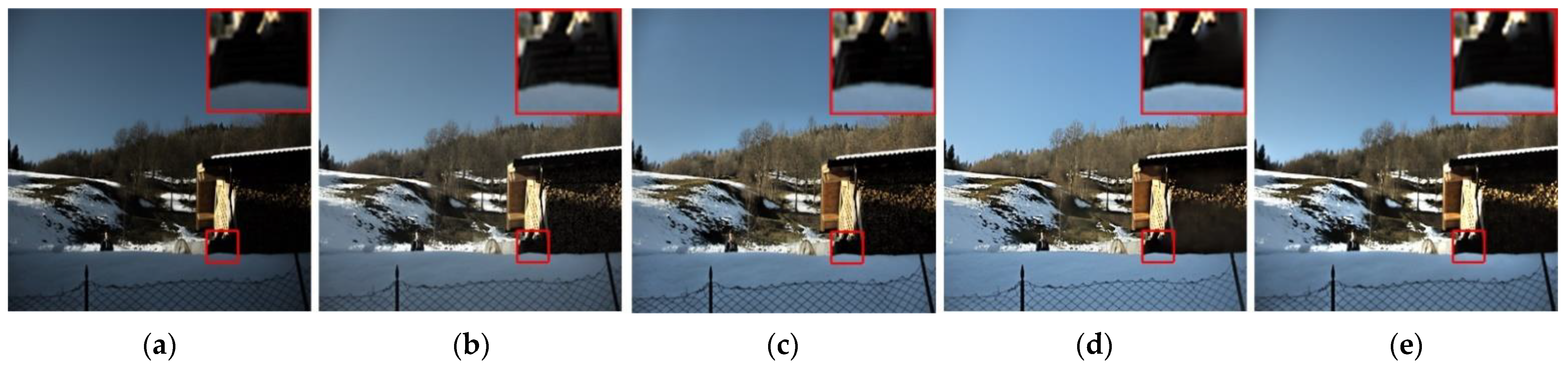
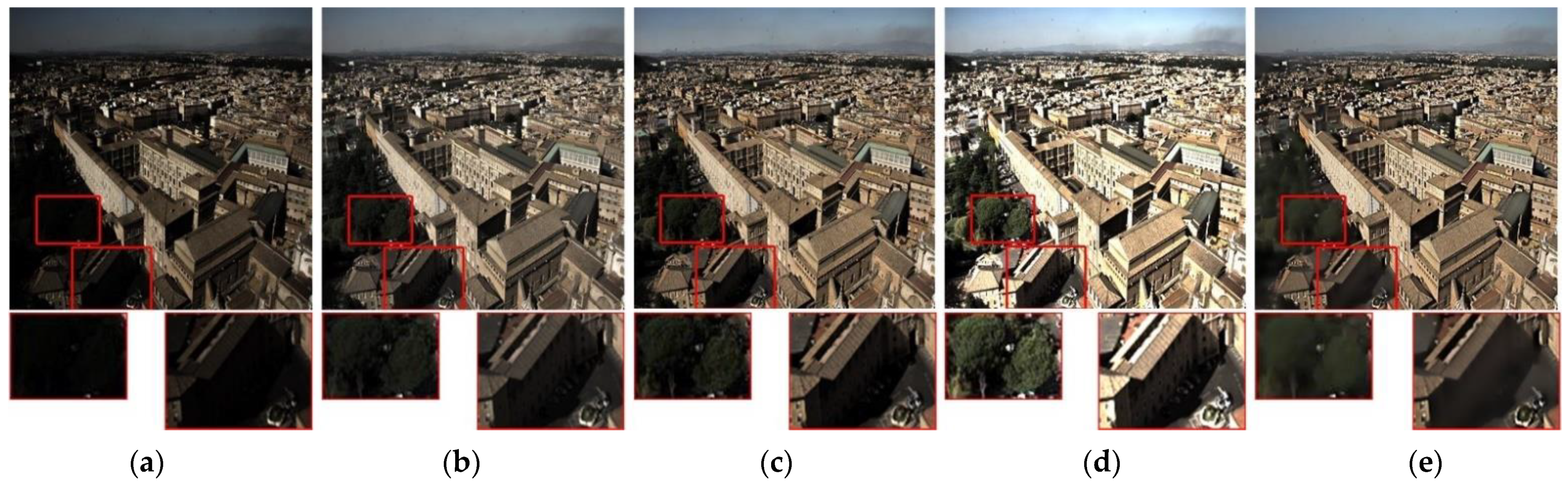
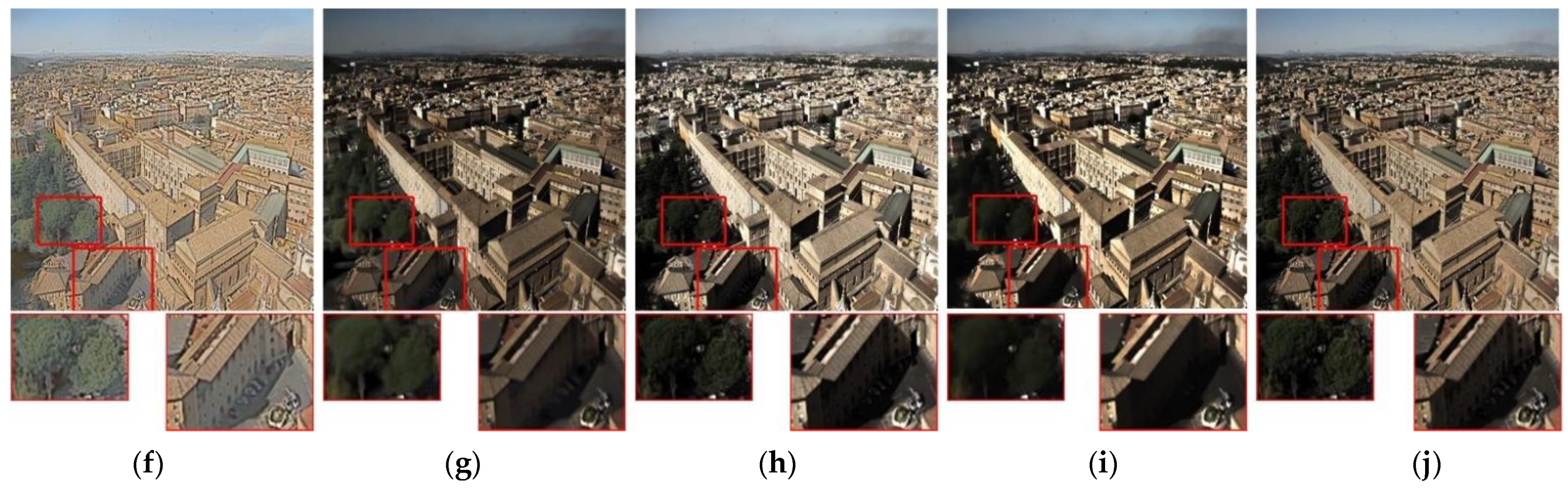
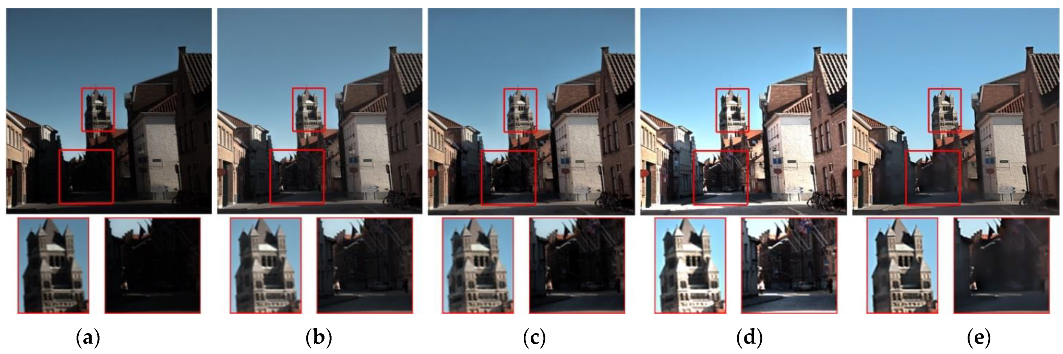
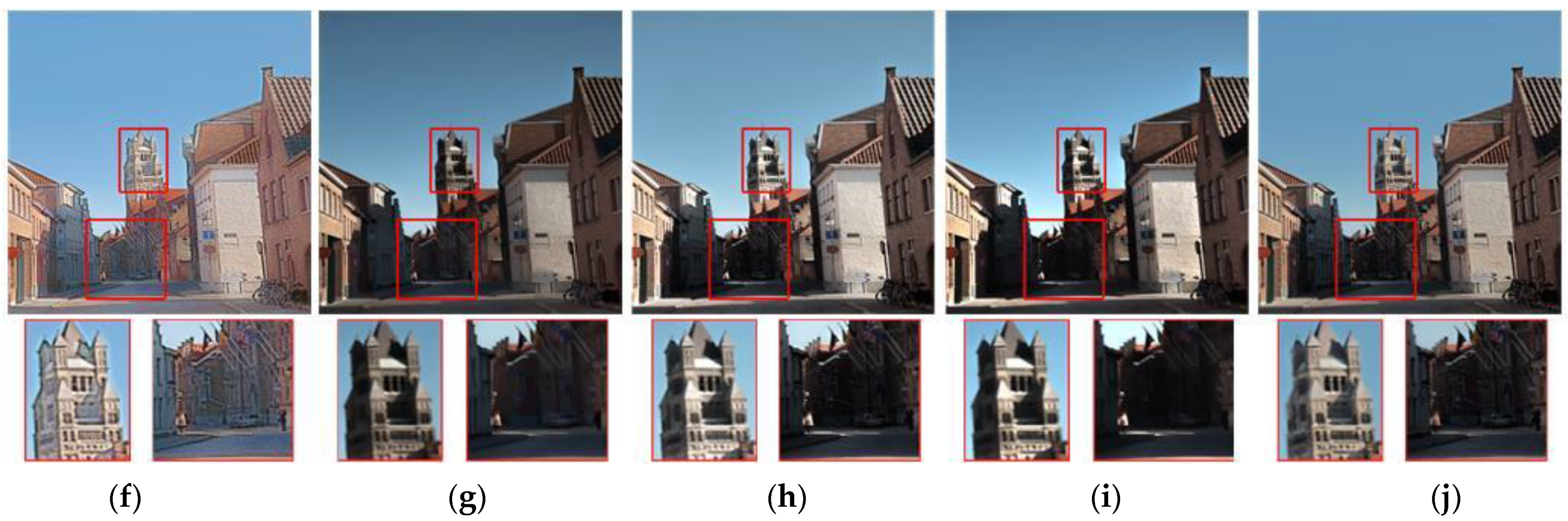
The initial illumination component and reflection component were obtained in Section 3.1. This section mainly improves the illumination component in terms of both brightness and contrast. For the problem of image brightness enhancement, the existing image enhancement algorithms have limited ability to enhance the darker regions. These include methods such as the bio-inspired multi-exposure fusion framework (BIMEF) [45], MF, structure-revealing low-light image enhancement via robust retinex model (SR) [46], and low-light image enhancement with semi-decoupled decomposition (SDD) [47], with results shown in Figure 4. The brighter areas are over-enhanced, resulting in blurred details with some methods, such as BIMEF, low-light image enhancement via illumination map estimation (LIME) [48], low-light image enhancement using the camera response model (LECARM) [49], and SDD, with results shown in Figure 5.
To solve the above problems, we designed the BEF function in two directions, as detailed in Section 3.2.1. The adaptive contrast enhancement (ACE) method improves the contrast by combining the high-frequency information of the image, but the high-frequency component is often doped with noise. Therefore, we devised a form of piecewise function to improve the image contrast pixel by pixel, as detailed in Section 3.2.2. The design of the fusion weight and Gaussian Laplacian pyramid are explained in Section 3.2.3 and Section 3.2.4, respectively.
3.2.1. Brightness Enhancement of Illuminance Map
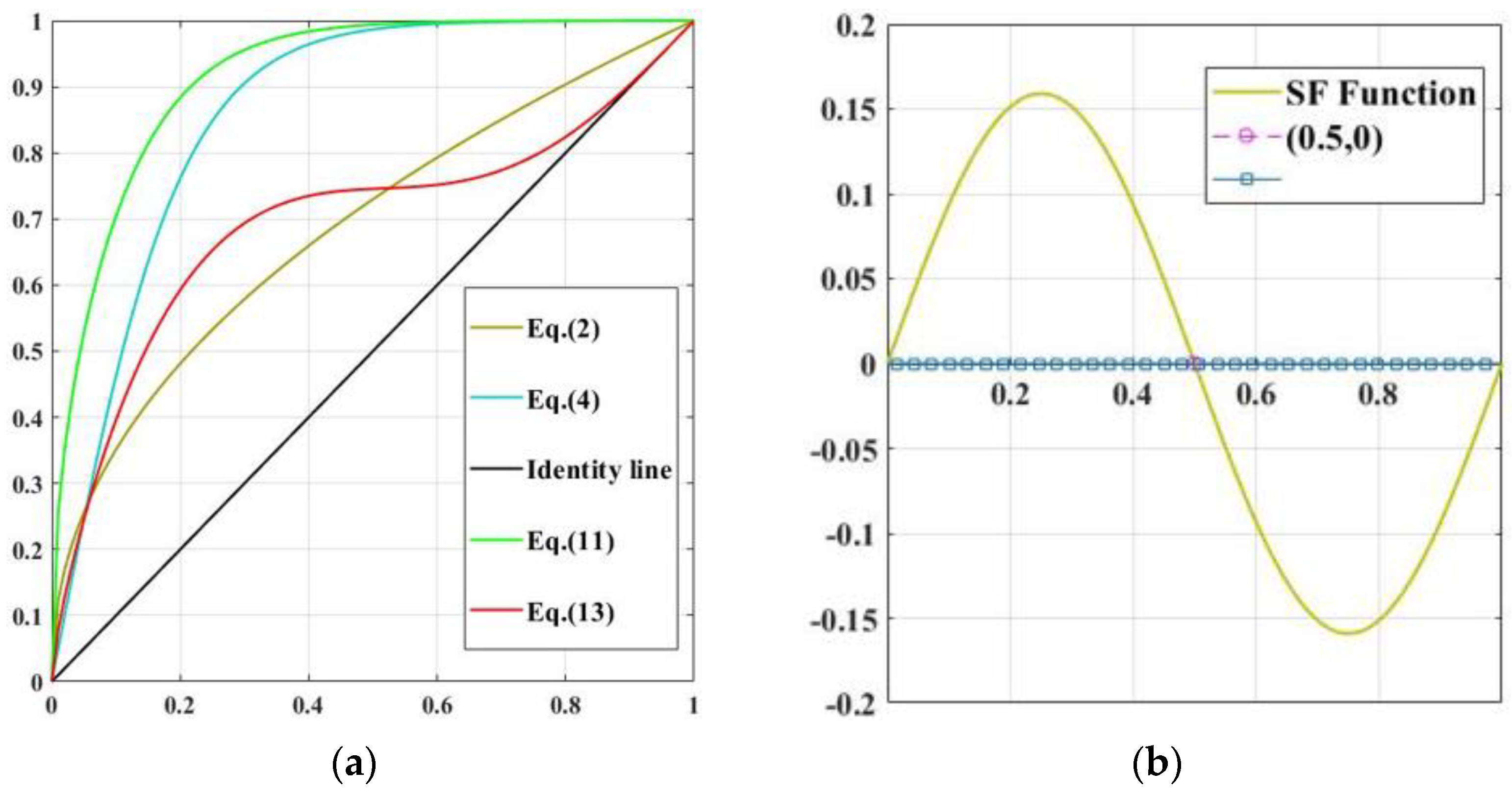
This section designs the BEF function by analyzing several brightness enhancement functions given in Section 2.2. Figure 6 shows two graphs for the different transformation functions, and the values of Equations (2) and (4) at any point are higher than the identity line, indicating that the pixel value at any point of the enhanced image is higher than that of the original image.
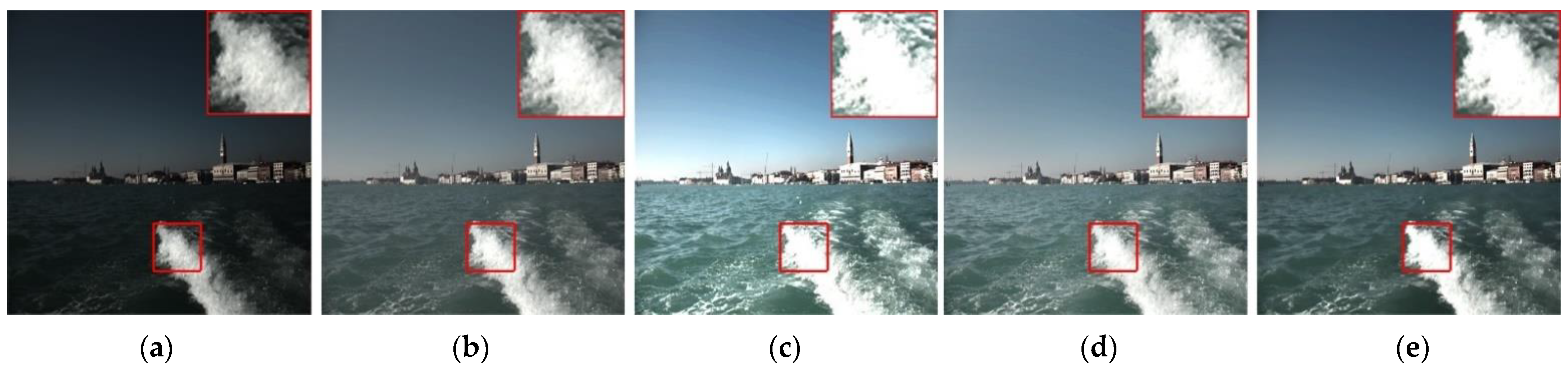
Figure 7 displays one raw low-light image and its counterparts enhanced by different transform functions. Both GC (2) and truncated normalized sigmoid (4) can enhance the brightness of the image. However, Equation (4) has limited enhancement ability for dark regions marked by red boxes, as shown in Figure 7c. Observing the curves of each formula in Figure 6a, it is found that GC (2) has the greatest enhancement in the region of low pixel value. Therefore, we can hopefully enhance the brightness details simultaneously for dark regions by cascading GC (2) and sigmoid (4) as follows:
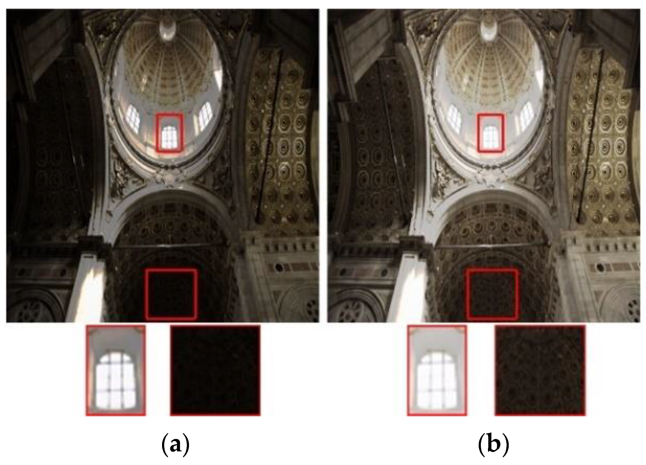
Figure 7d shows the image enhanced by Equation (11), which is better than Equations (2) and (4). However, for the window area in the red box of the image, Equation (11) produces overexposure, resulting in complete loss of image content. This is due to the fact that in the high-pixel value region, the curve of Equation (11) is much higher than the identity line in the high-pixel value region, as shown in Figure 6a. Inspired by the characteristics of the sine function (SF), in which the values are greater than 0 between [0, 0.5] and less than 0 between [0.5, 1], as shown in Figure 6b, we accordingly considered adding the SF function to the original image to suppress the bright areas in the image. We designed the following transform function:
where
It is obvious that we have for , while for .
Obviously, the enhancement result of Equation (12) can retain more details as shown in Figure 8a, but the whole image is dark. In order to further improve the visual quality, we combine Equations (11) and (12) to obtain the first image for fusion:
So far, we have completed the luminance improvement of the illuminance map through Equation (13).
The corresponding plot of Equation (13) is shown in Figure 6a, where the entire curve is almost always above the identity line with the first part of the curve being significantly higher than the identity line, due to the need for greater enhancement in the low pixel value region. However, it almost coincides with the line near 1, indicating that there is almost no enhancement here, so that over-enhancement can be avoided. Figure 8b shows the enhanced result with Equation (13). As can be seen, the resulting image not only improved the brightness, but also was not overexposed. It is clearly better than that obtained with Equation (12).
3.2.2. Contrast Enhancement of Illuminance Map
Improving image contrast is also an important step to enhance low-illumination images. The adaptive contrast enhancement algorithm (ACE) to enhance the high-frequency component is a classical method [50]. The specific formula is:
where and are the i-th pixel of the original image and the corresponding enhanced image.
where and are the mean and variance of the local windows , respectively. We set in this paper.
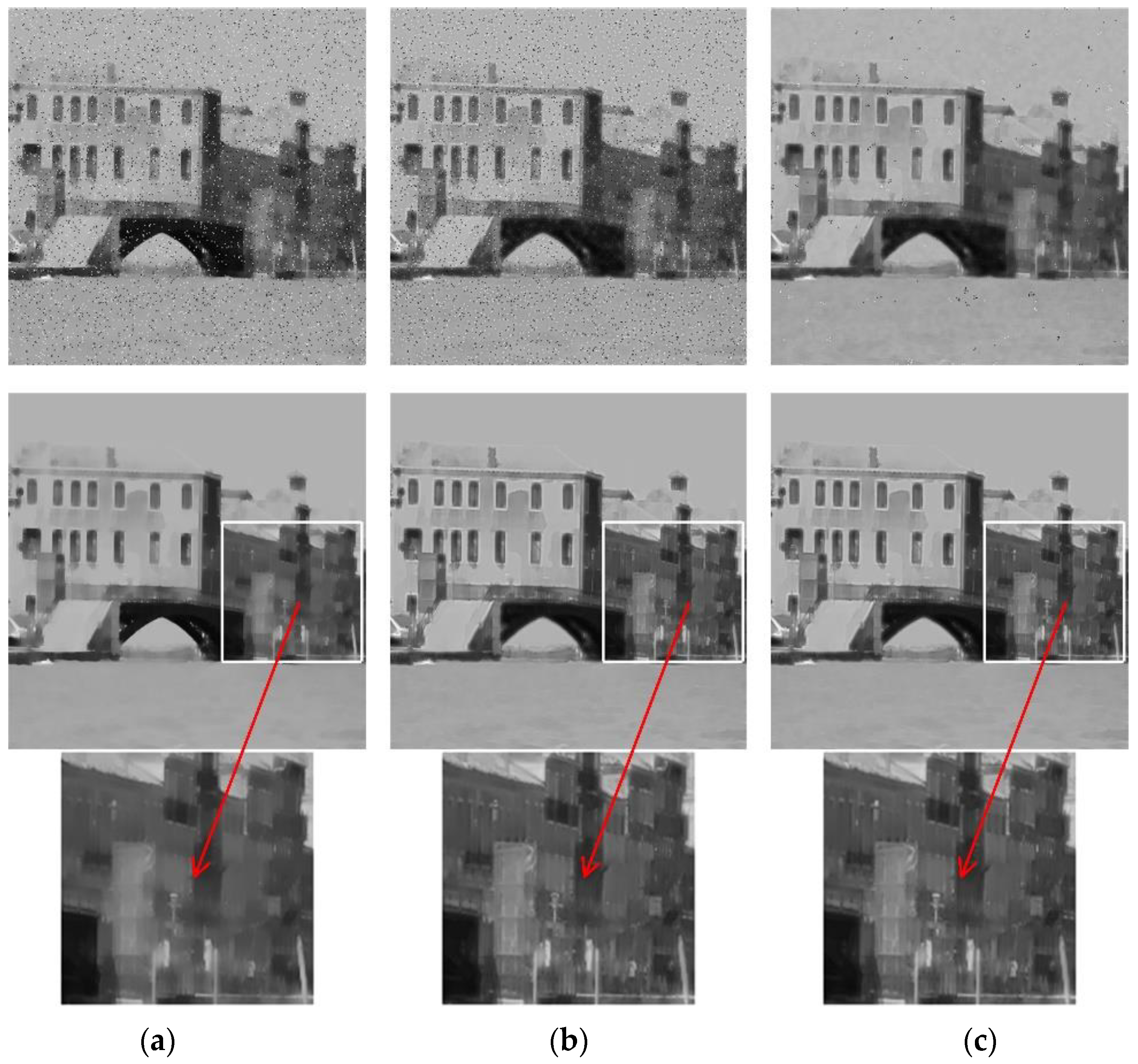
As is known to all, the noise is regarded as a point whose pixel value is significantly different from other pixels in the local area, which belongs to the high-frequency part. Therefore, the ACE algorithm can easily amplify the noise while improving contrast. To solve this problem, we sought to determine whether any pixel is noisy or not and then update its value in two corresponding ways. Specifically, when a pixel is not a noisy point, its value is still updated according to ACE (14), and conversely, its value is replaced with the mean and variance of the local area after removing all noisy points. The whole updating rule for improved ACE (IACE) is as follows:
where and are the mean and variance of the i-th window after removing noisy points, respectively. The mean ensures the overall information of the local area, and the variance takes into account the difference information between pixels This simple criterion maintains the difference value between pixels and does not blur the image. The final image obtained from (15) is the second input image () for fusion, where , represents the number of elements in the set. For the local area with the size of , the experiment shows that if is defined as the noise point, the experimental effect is the best. Of course, can be adjusted according to the size of the local area; in this paper, .
Figure 9 shows the contrast enhancement results achieved with Equations (14) and (15). For the noisy image shown in the first row, we can see that IACE can eliminate most of noise compared to ACE. For the noise-free images shown in the second row, we can see that IACE can improve contrast and sharpness. In other words, IACE can significantly improve contrast and eliminate noise at the same time.
3.2.3. Design of Fusion Weights
In order to combine the advantages of the two images, the Gaussian–Laplacian pyramid algorithm is used to fuse the two input images obtained above, and the fusion weights are composed of brightness weight and detail weight. This section mainly introduces two kinds of weights.
In order to have a natural brightness, we adopt a global brightness weight for the k-th input image as in [27]:
As pointed out in Section 2, the gradient and variance are important for image details. In order for the enhanced image to contain rich content, the detail weight is designed as follows:
is the normalization factor, where
where and are the gradients of the local patch in direction and direction, respectively, and is the variance of the local region. is the summation of the variance and the gradient, indicating the amount of information in the local area. To ensure that the value of is between [0, 1], needs to be normalized. So, the larger the , the higher the weight value and information contained in the image.
The final weight is obtained by:
where
3.2.4. Gaussian Laplacian Pyramid Fusion
In order to obtain a refined illumination map, we use the Gaussian–Laplacian Pyramid method [51] to fuse two input images obtained from Equations (13) and (15) with the fusion weights from Equation (20). We decompose either input image into a Laplacian pyramid to extract image features and decompose either normalized weight into a Gaussian pyramid to smooth strong transitions [27]. Then, we fuse these pyramids by mixing each layer, and the final enhanced illumination map is obtained by summing up-sampling on the fused pyramids:
where is the up-sampling operator with factor ( is the number of layers of the pyramid; we select ), and and are the Laplacian decomposition and Gaussian decomposition, respectively.
3.3. Image Enhancement Based on the Retinex Theory
According to retinex theory, the adjusted illumination map is multiplied by the reflection component from Equation (10) to obtain the final enhanced image:
4. Experiments and Results
In this section, we verified the performance of the proposed method. All experiments were conducted using Matlab R2018a on a PC with a 3.60 GHz Intel Pentium Dual Core Processor and 16.0 G RAM.
We performed qualitative and quantitative comparisons with the state-of-the-art algorithms. They included BIMEF [45], MF [27], LIME [48], SR [46], Ret-Net, FFM [28], LECARM [49], and SDD [47]. Several datasets such as MF [27], Fusion [29], LOL dataset [33], LIME [48], NPE [52], DICM [53], Synthetic dataset [33,54], and SRIE [55].
For evaluating the proposed method’s performance, five no reference image quality assessment (NIQA) metrics, including the natural image quality evaluator (NIQE) [56], the blind/reference-less image spatial quality evaluator (BRISQUE) [57], the colorfulness-based patch-based contrast quality index (CPCQI) [58], the integrated local NIQE (IL-NIQE) [59], and the no-reference free energy-based robust metric for contrast distortion (NIQMC) [60], and one full reference IQA metric, that is, the patch-based contrast quality index (PCQI) [61], were used for quantitative evaluation.
4.1. Subjective Evaluation of Experimental Results
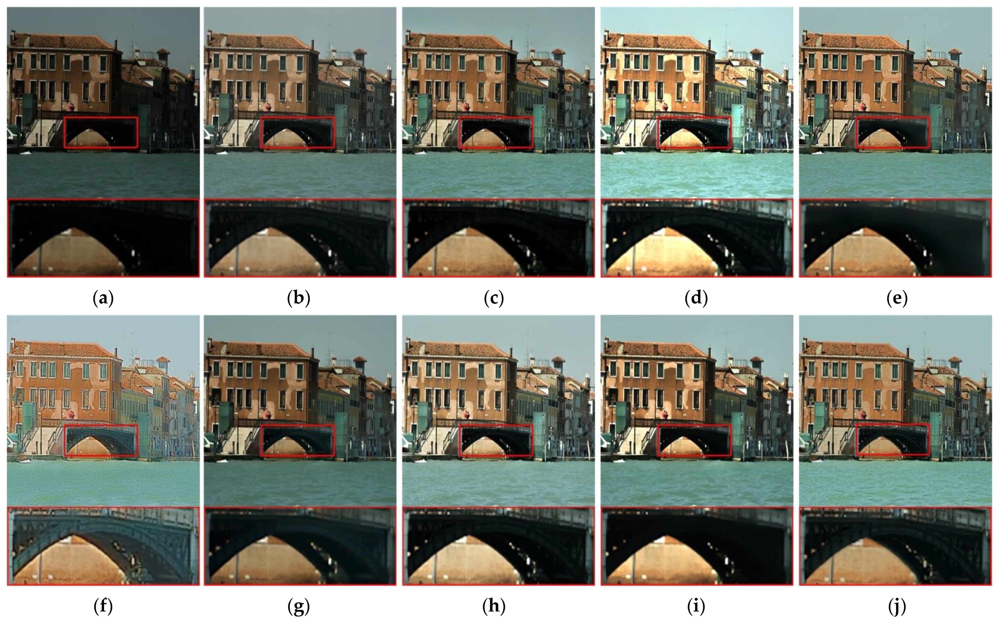
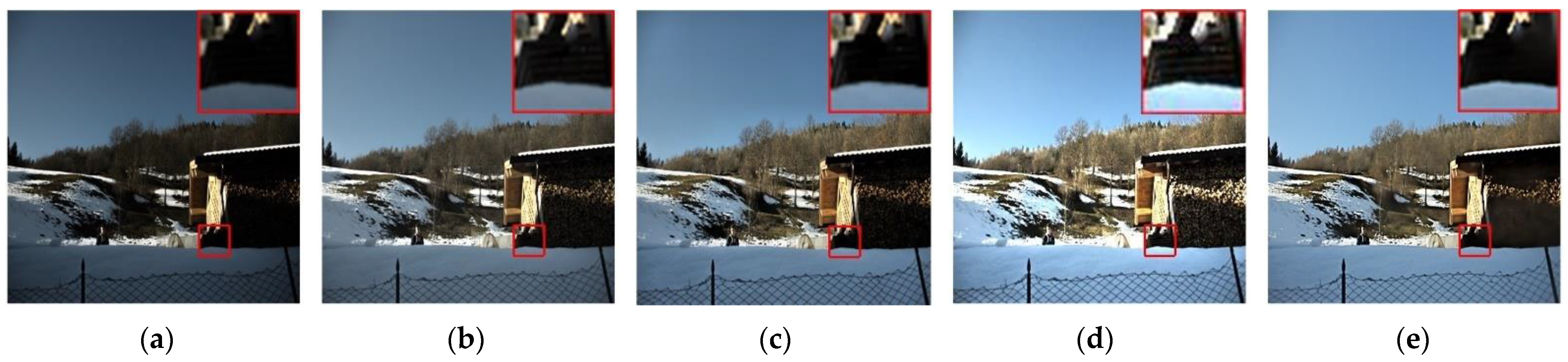
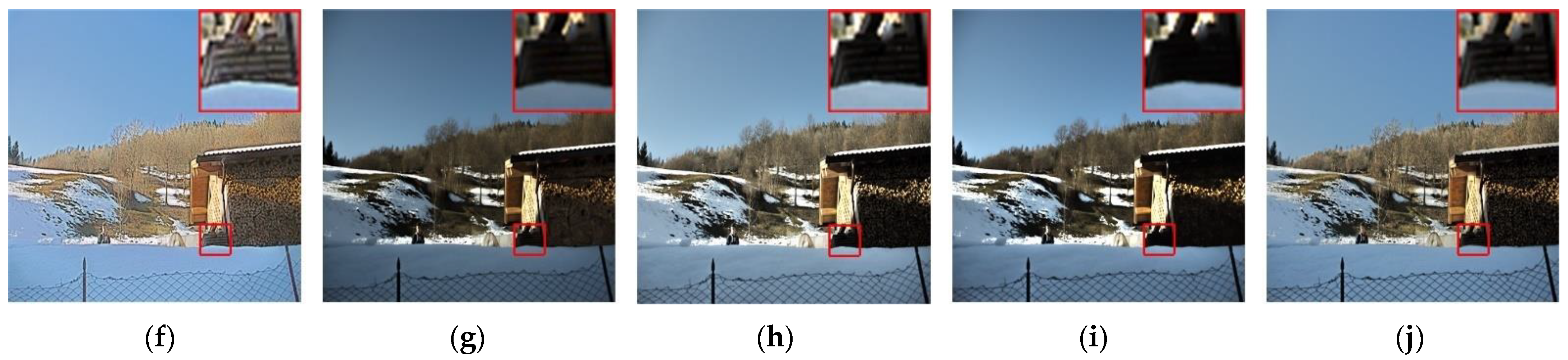
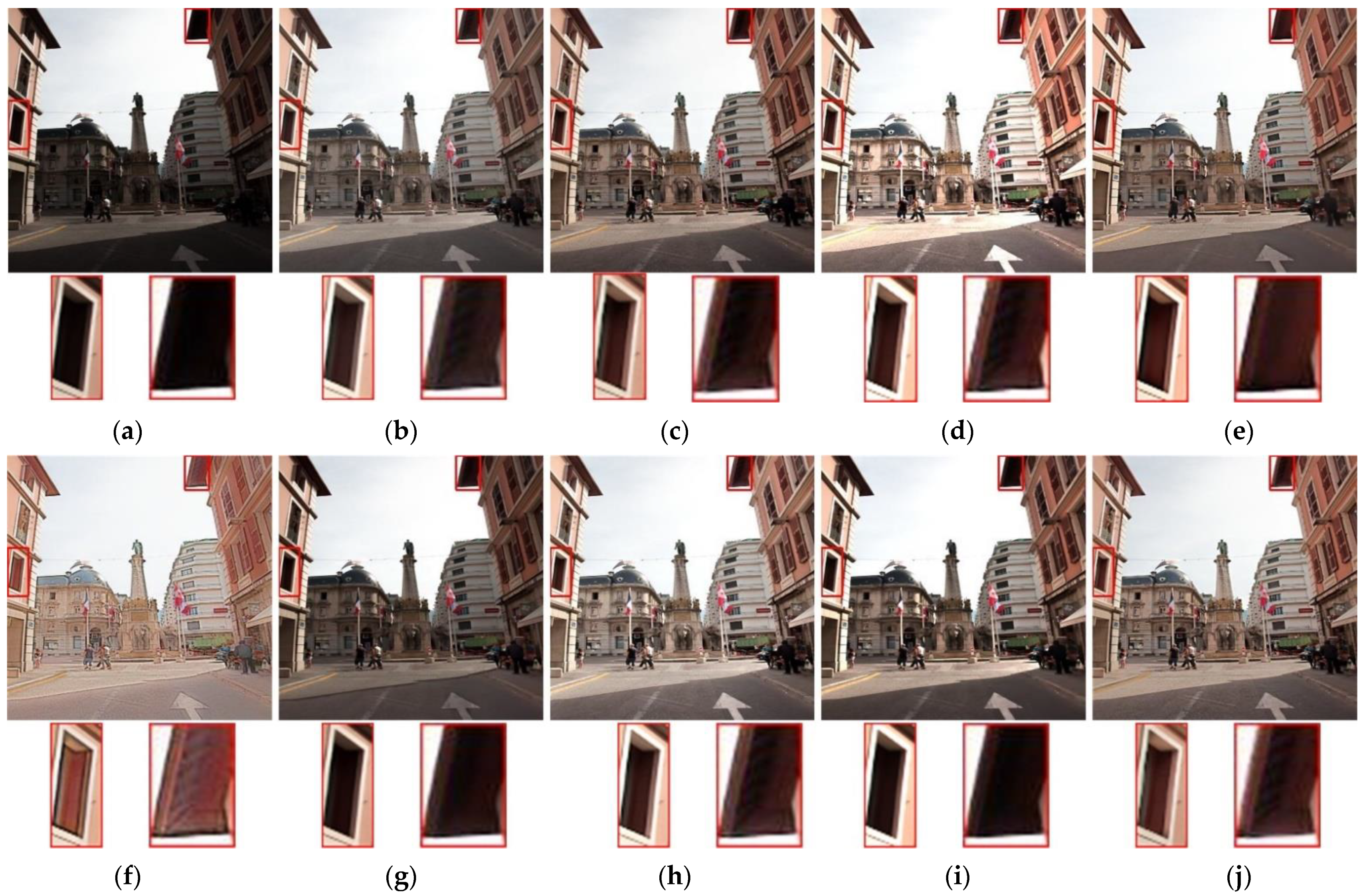
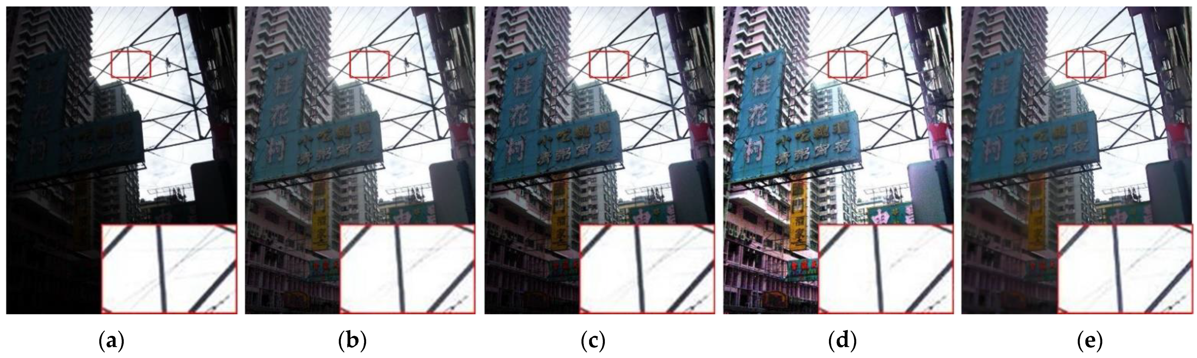
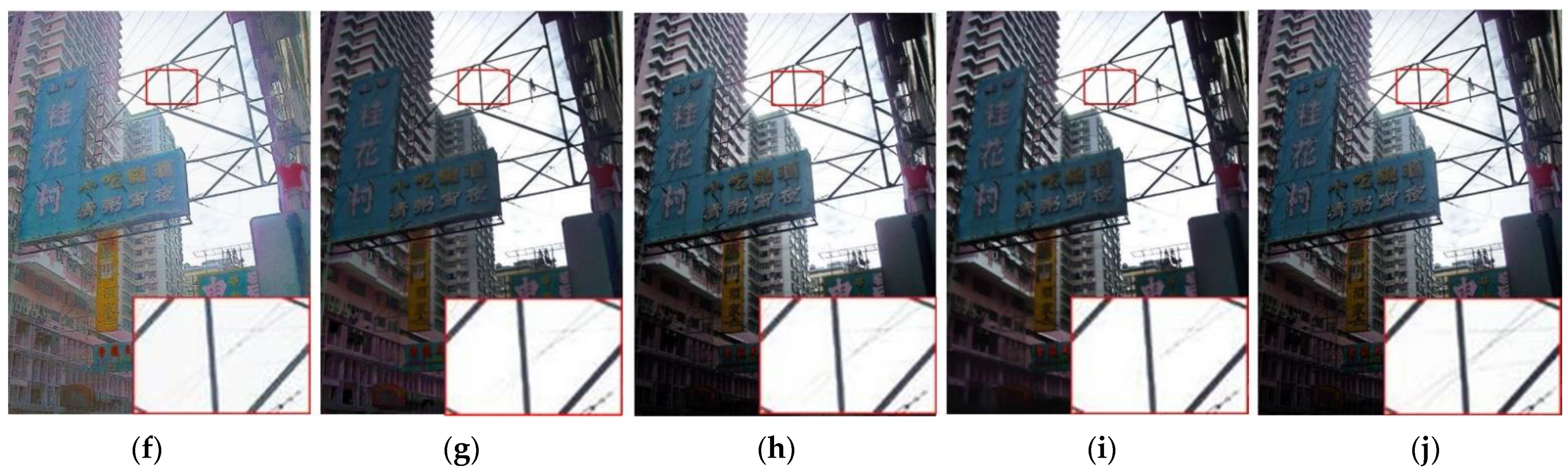
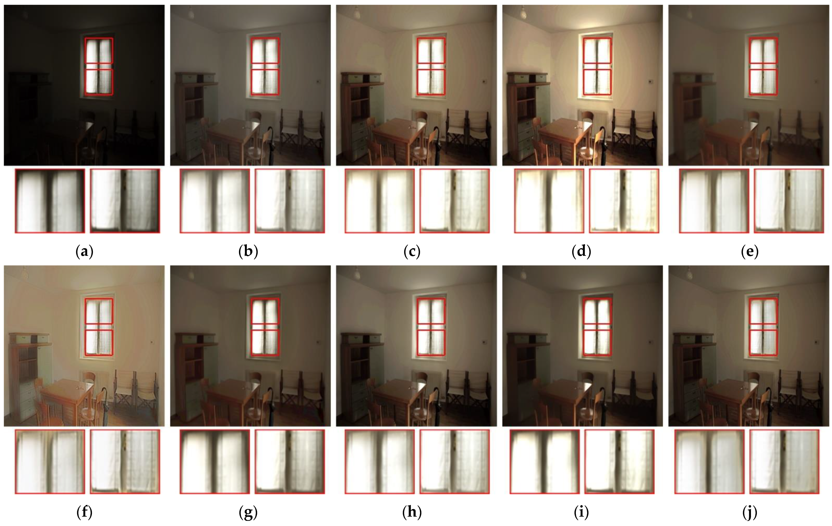
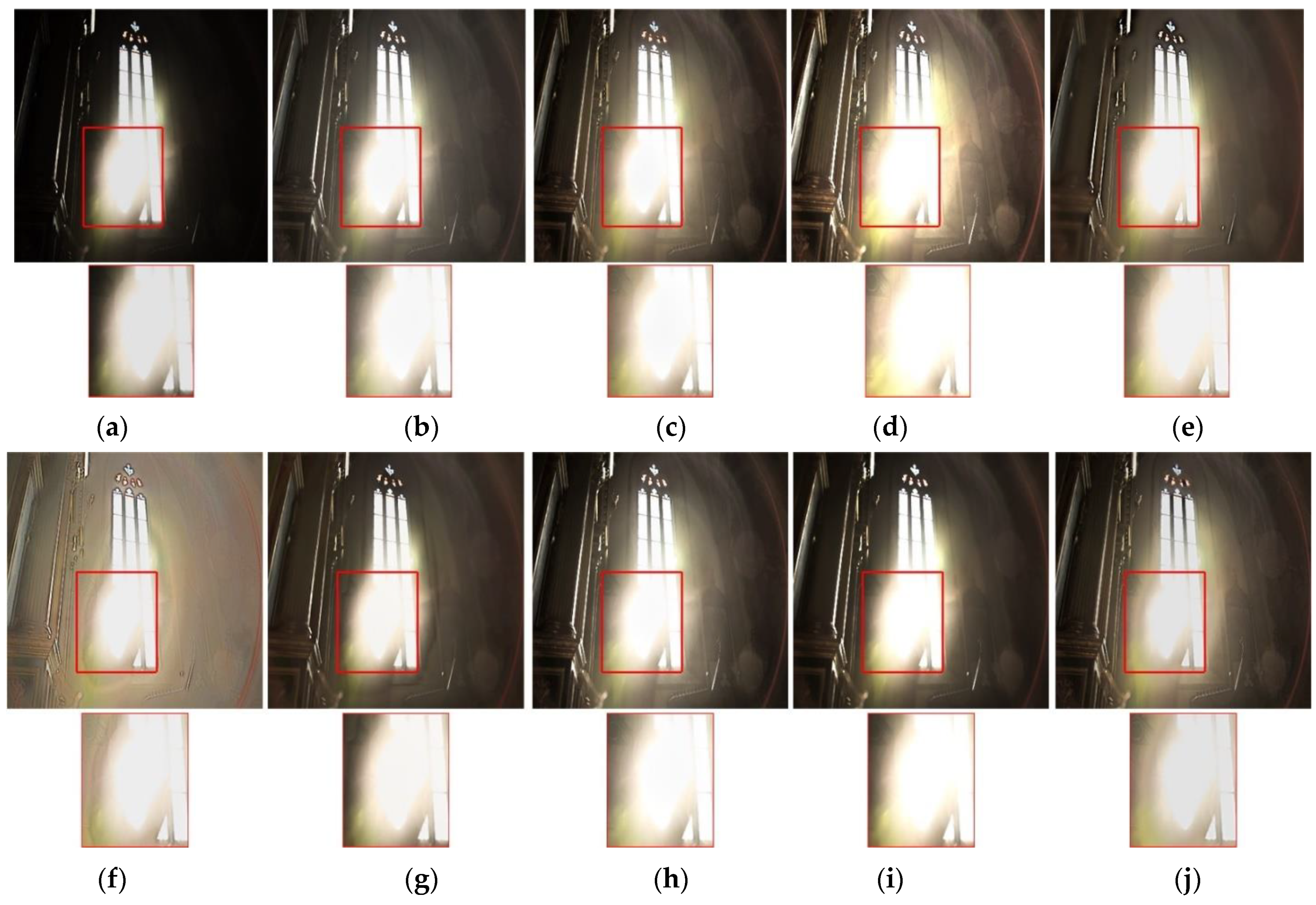
In this section, we analyzed the effectiveness of the proposed method from a subjective perspective for the darker and lighter areas of the image. As shown in Figure 10, Figure 11, Figure 12, Figure 13, Figure 14 and Figure 15, six images, i.e., “Bridge”, “House”, “Window and Eave”, “Plant and Shadow”, “Tree”, and “Town” were used to illustrate that the proposed method can commendably reveal dark areas. As shown in Figure 16, Figure 17, Figure 18, Figure 19, Figure 20, Figure 21 and Figure 22, another seven images, i.e., “Girl”, “River”, “Shoes”, “Street”, “Window curtain”, “Hand”, and “Church” were used to illustrate that the proposed method does not produce overexposure, while increasing overall brightness and retaining more details.
4.1.1. Testing the Effectiveness of the Proposed Method in Dark Regions
The overall pixel values of shimmering images were small, and there were often completely dark areas in the images, such as the bridge in Figure 10, the wooden stakes in the corner of the house in Figure 11, the eave in Figure 12, and so on. As shown in Figure 10, Figure 11, Figure 12, Figure 13, Figure 14 and Figure 15, all methods improved the brightness of the image to a certain extent, but the red box areas of the image were enhanced differently.
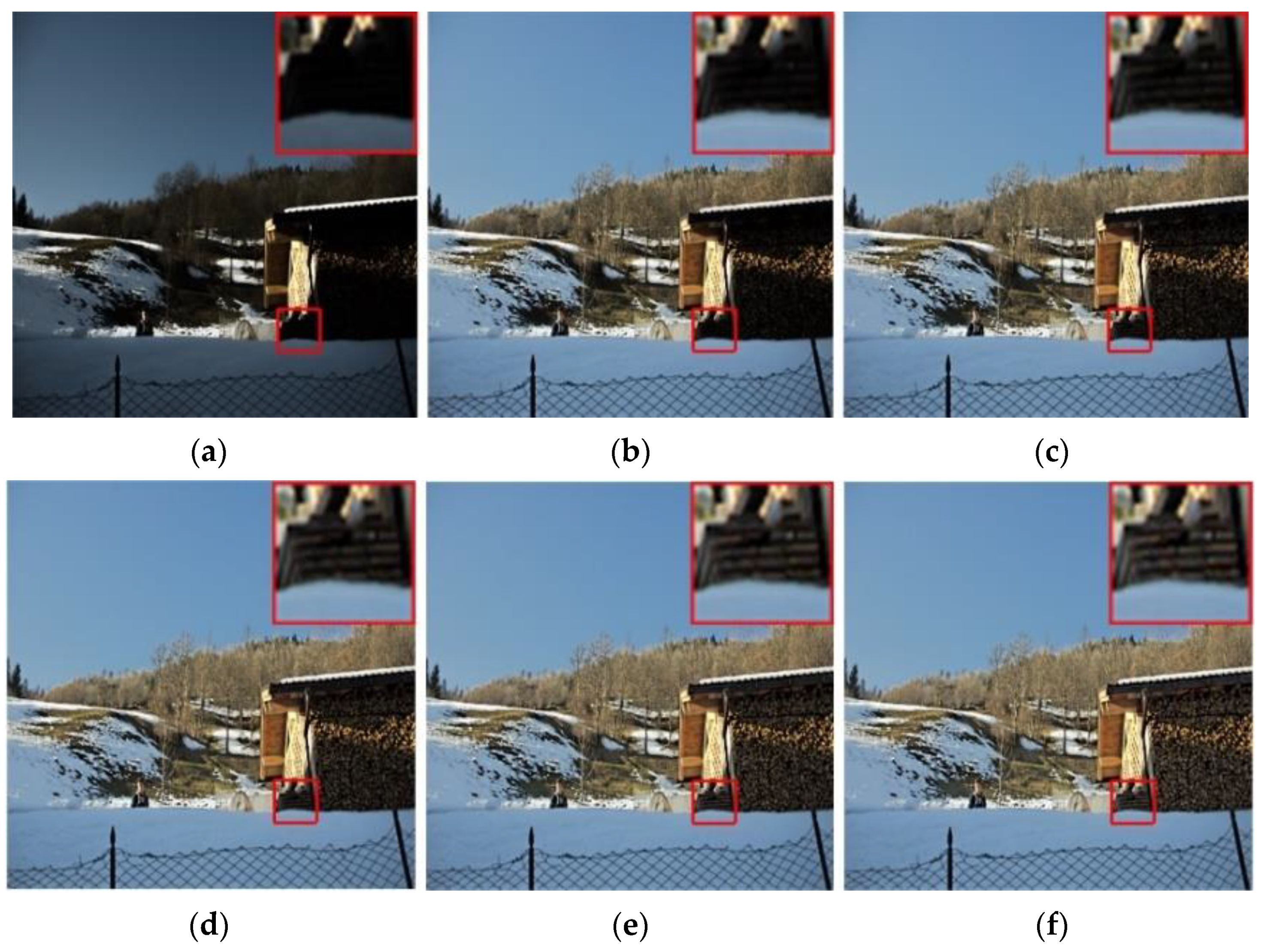
For instances, for the red frame region in Figure 11, some methods (i.e., MF, LIME, FFM, and LECARM) had less visible enhancement, while some methods (i.e., BIMEF, SR, and SDD) had little or no effect. The dark region enhanced by Ret-Net could be clearly seen, but its details were also blurred. Our proposed method had a significant effect for recognition of the wooden stake. This was because addition of GC to the BEF function improved the enhancement of dark areas. Similarly for Figure 15, for the roof in the red frame, some methods (e.g., BIMEF, SR, Ret-Net, FFM, SDD) blurred details, whereas LIME and LECARM led to different degrees of over-enhancement. The enhancement effects of MF and the proposed method were obviously better than those of the other algorithms. However, in the area of the square box, the proposed method showed relatively clear content.
4.1.2. Testing the Effectiveness of the Proposed Method in Bright Regions
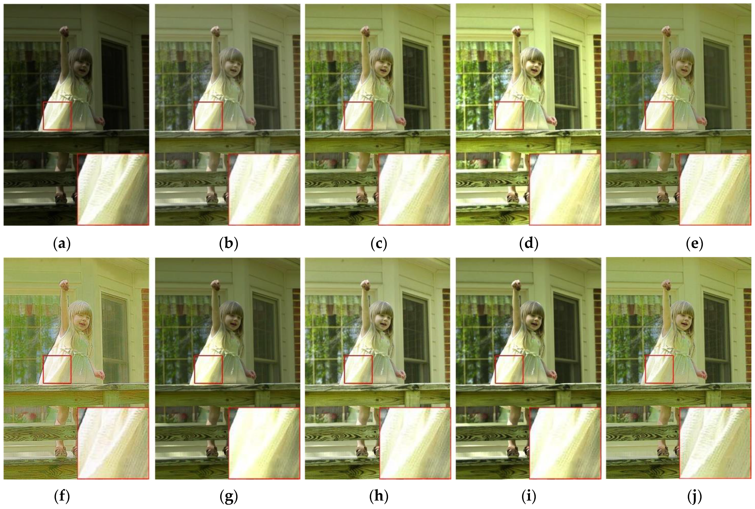
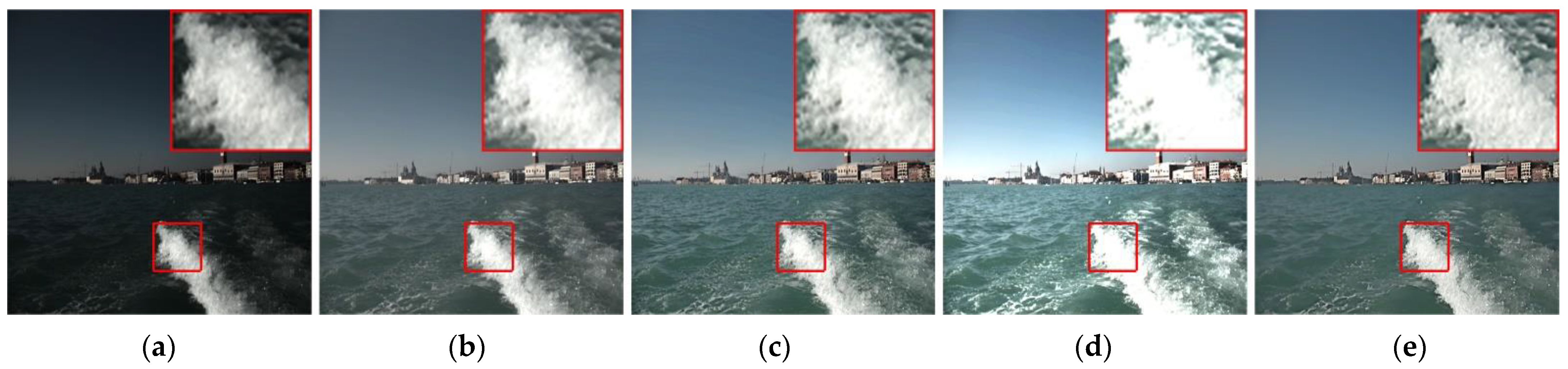
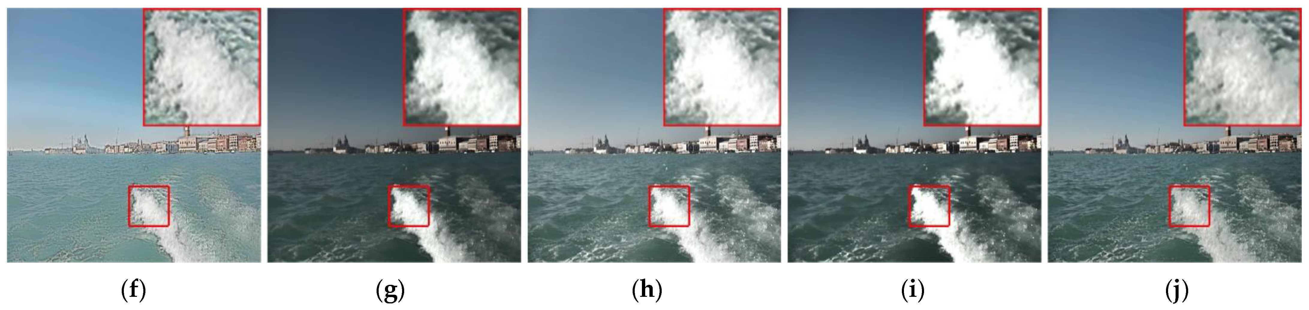
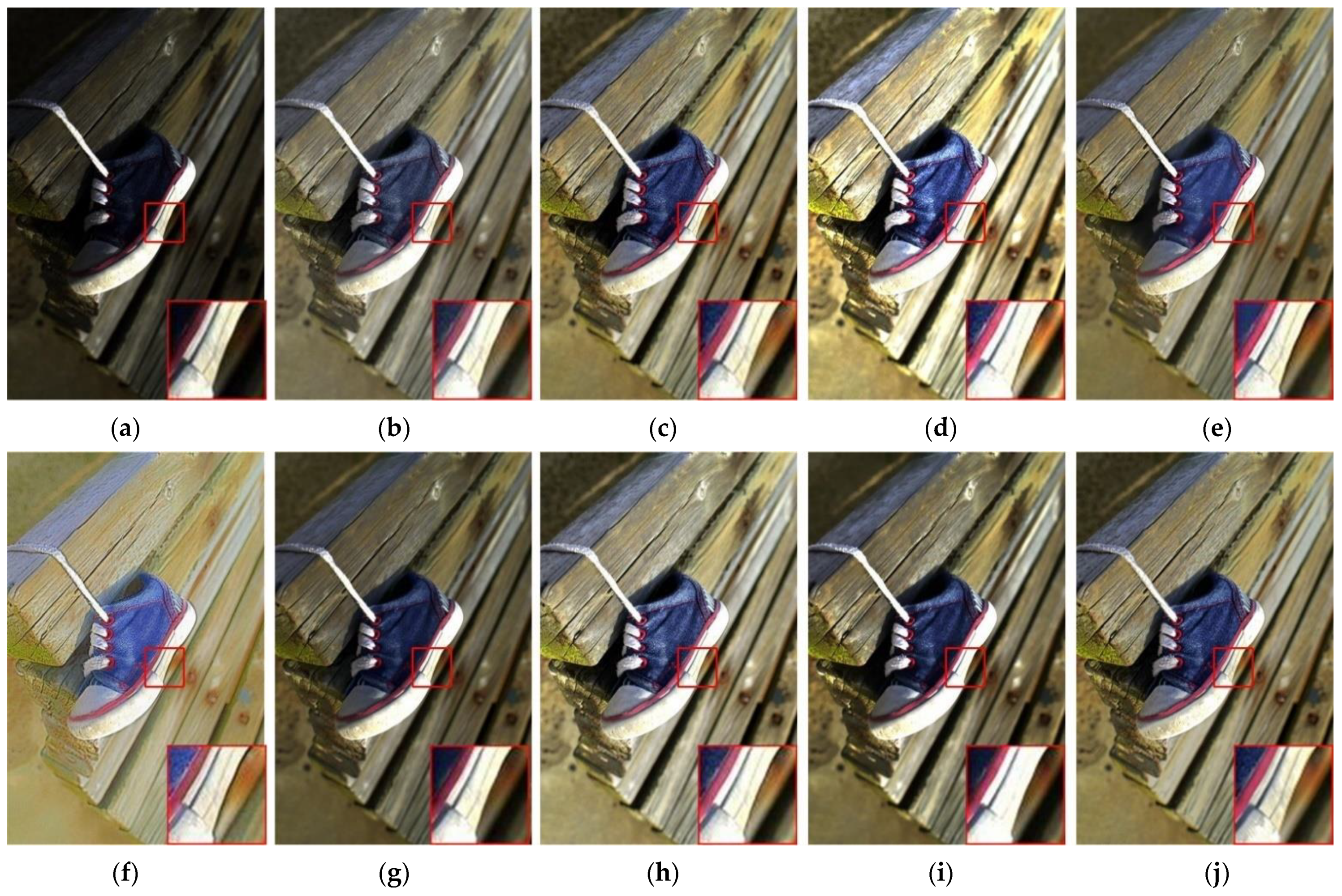
For the highlighted areas close to the light sources in the images, the pixel value was generally high. Examples include the girl’s dress in Figure 16, the river in Figure 17, the hand in Figure 21, etc. These areas were inherently highly brightness and did not require much enhancement. Figure 16, Figure 17, Figure 18, Figure 19, Figure 20, Figure 21 and Figure 22 show the enhancement results of all comparison algorithms and the proposed method on different images. For high pixel value areas, each comparison algorithm caused a different degree of blurring, while the proposed model retained more complete information.
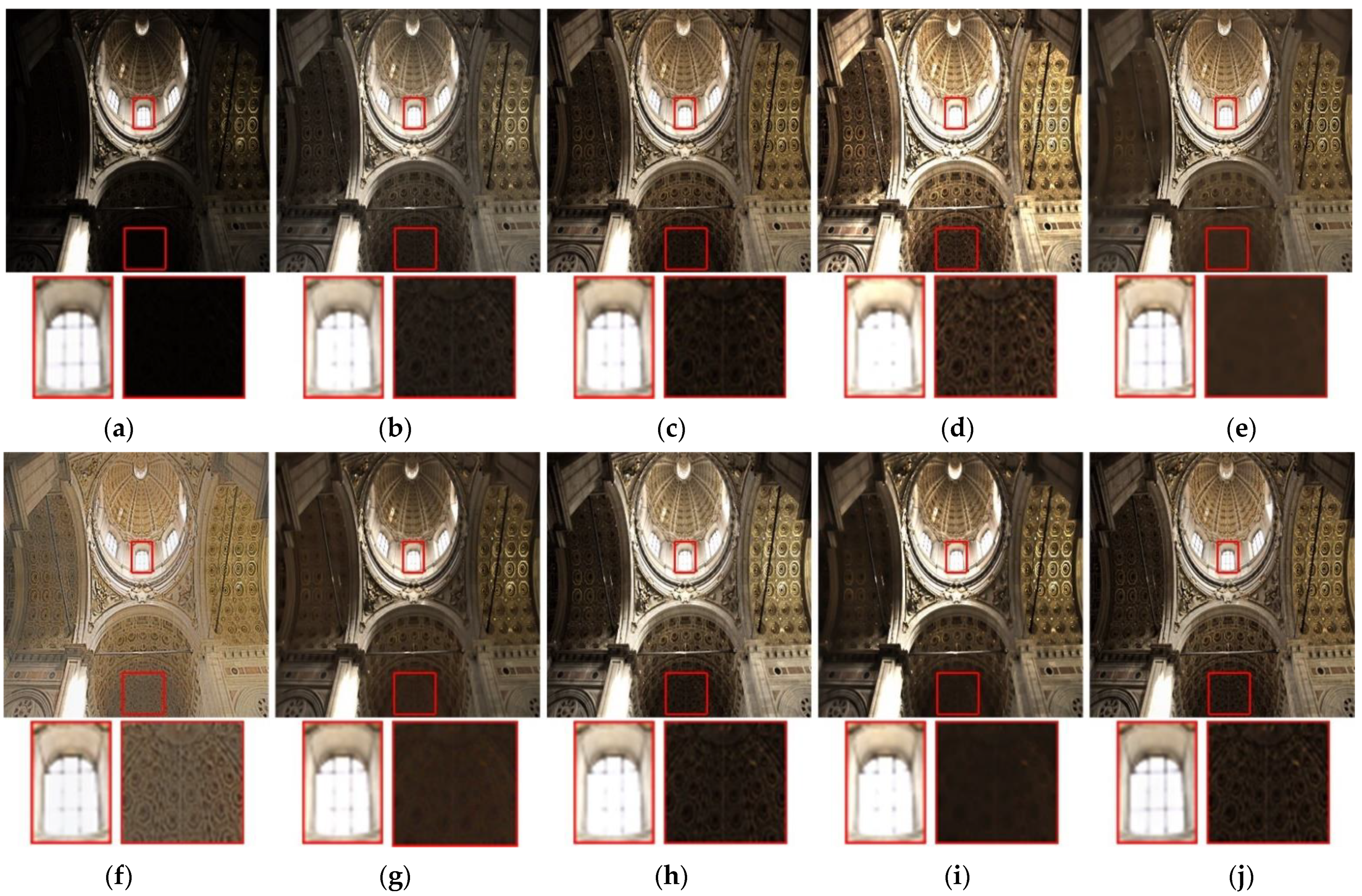
For example, in Figure 16, for the skirt in the red box area, BIMEF, MF, LIME, SR, FFM, LECARM and SDD adopted the same strategy for all areas when enhancing the image, regardless of the pixel values of the image itself, resulting in excessive exposure and blurred image details. The BEF transform function of our proposed method enhanced the brighter region slowly or not, and was able to improve the image brightness while maintaining the detail information, so the content in the region could be preserved completely. In Figure 22, the window above the church had a high pixel value and, therefore, did not require much enhancement. However, BIMEF, MF, LIME, SR, FFM, LECARM and SDD were enhanced for every pixel value of the whole image, thus losing some information. The method proposed in this paper retained the original content of the window area to a large extent.
4.2. Objective Quality Assessments
To quantitatively evaluate the performance of the proposed method, we performed a full-reference evaluation and a non-reference evaluation. Specifically, we used 104 images from different datasets for comparative experiments. These images were composed of two parts, a total of 13 images from Figure 10, Figure 11, Figure 12, Figure 13, Figure 14, Figure 15, Figure 16, Figure 17, Figure 18, Figure 19, Figure 20, Figure 21 and Figure 22 and 91 other images, respectively. The average values of the corresponding quantitative indicators are shown in Table 1, and the best indicators are shown in bold. Where, (↑) means that the larger the value, the better, and (↓) is the opposite.
(1) Non-Reference Evaluation: We employed five non-reference metrics, that is, NIQE, BRISQUE, CPCQI, IL-NIQE, and NIQMC, for low-light image quality evaluation.
NIQE constructs a “quality-aware” collection of statistical features based on the Natural Scene Statistics (NSS) model in the spatial domain. BRISQUE uses NSS with locally normalized luminance coefficients to quantify the possible loss of “naturalness” in order to assess the overall image quality. CPCQI uses a regression module to generate visual quality metrics by analyzing 17 features such as contrast, sharpness, and luminance. IL-NIQE learns multivariate Gaussian models of image blocks by integrating statistical features from multiple natural images. Additionally, the Bhattacharyya-like distance is used to measure the quality of each image block, and the overall quality score is obtained by averaging pooling. NIQMC combines local and global determination of which image has greater contrast and better quality between two images. The lower the values of NIQE, BRISQUE, and IL-NIQE, the higher the image quality is, while higher scores for CPCQI and NIQMC mean that a better contrast is obtained than the reference image.
As shown in Table 1, the proposed method had the optimal NIQE and CPCQI values, with the BRISQUE value and IL-NIQE ranking second and NIQMC ranking fourth. This means that the results of the proposed method were more consistent with human vision, and the contrast was in the middle position.
(2) Full-Reference Evaluation: We conducted a full-reference evaluation using the PCQI metric. PCQI decomposes the image block into mean intensity, signal intensity and signal structure components and evaluates the perceived distortion of these components separately. A higher PCQI denotes that the result has higher visual effect and quality. As shown in Table 1, our proposed method stood out as the best performer.
This part verified the effectiveness of our method from two aspects: full reference and non-reference. Although not every index had the best results, the model outperformed other algorithms overall.
5. Limitations and Discussion
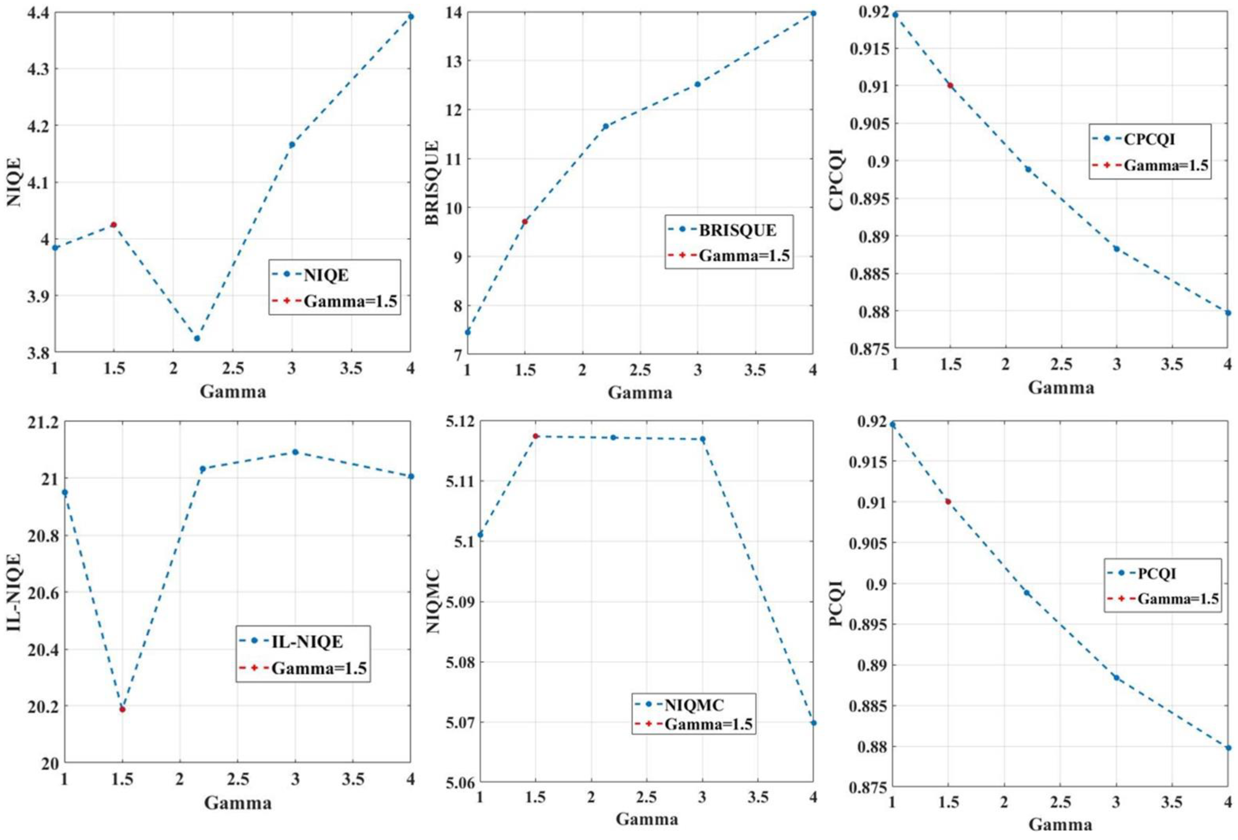
There are still some deficiencies in the model proposed in this paper. (1) When selecting the value of Equation (11), we found that the larger the was, the more obvious the dark area detail was, as shown in Figure 23. The quantitative index in Figure 24 almost reached the optimal value when , but it could not display the content of the dark area. Therefore, how to balance the selection of and quantitative indicators is a problem to be studied in the future. (2) With the continuous development of deep learning, using a convolutional neural network to improve low-light images will be our key research direction.
6. Conclusions
In this paper, we presented a simple yet efficient retinex-based method for low-light images. The research mainly included the following steps: firstly, an initial illumination map estimation algorithm based on neighborhood information was proposed. Then, in order to further enhance brightness and local contrast of the initial illumination map, two input images, which were obtained by BEF and IACE, respectively, were fused by means of the Gaussian–Laplacian pyramid. Finally, the enhanced image was obtained based on retinex theory. Images from different datasets were used to verify the effectiveness of our method from both subjective and objective aspects, that is, our method can not only improve the brightness, but also retain more detailed information. In the future, we aim to enhance low light images by extracting rich image features in conjunction with the currently hotter deep learning.
Author Contributions
Conceptualization, X.P. and C.L.; methodology, X.P., C.L., Z.P. and J.Y.; software, X.P. and S.T.; validation, X.P. and S.T.; writing—original draft preparation, X.P.; writing—review and editing, C.L.; supervision, C.L. and X.Y.; funding acquisition, C.L. All authors have read and agreed to the published version of the manuscript.
Funding
This research was funded by the Startup Foundation for Introducing Talent of NUIST under grant No. 2022r081, the open fund of Guangdong Provincial Key Laboratory of Digital Signal and Image Processing Technology under grant No. 2020GDDSIPL-02, and in part by the National Natural Science Foundation of China under grant No. 61871174.
Institutional Review Board Statement
Not applicable.
Informed Consent Statement
Not applicable.
Data Availability Statement
Not applicable.
Acknowledgments
We would like to thank the anonymous reviewers for their valuable suggestions, which have helped us to improve the manuscript greatly.
Conflicts of Interest
The authors declare no conflict of interest.
References
- Wang, H.; Zhang, Y.; Shen, H. Review of image enhancement algorithms. Chin. Opt. 2017, 10, 438–448. [Google Scholar] [CrossRef]
- Mukhiddin, M.; Cho, J. Smart Glass System Using Deep Learning for the Blind and Visually Impaired. Electronics 2021, 10, 2756. [Google Scholar] [CrossRef]
- Fang, W.; Li, H.; Lei, L. A review on low light video image enhancement algorithms. J. Changchun Univ. Sci. Technol. 2016, 39, 56–64. [Google Scholar]
- Park, S.; Kim, K.; Yu, S.; Paik, J. Contrast enhancement for low-light image enhancement: A survey. IEIE Trans. Smart Process. Comput. 2018, 7, 36–48. [Google Scholar] [CrossRef]
- Zhu, J.; Li, L.; Jin, W. Natural-appearance colorization and enhancement for the low-light-level night vision imaging. Acta Photonica Sin. 2018, 47, 159–198. [Google Scholar]
- Faramarzpour, N.; Deen, M.J.; Shirani, S.; Fang, Q.; Liu, L.W.C.; de Souza Campos, F.; Swart, J.W. CMOS-based active pixel for low-light-level detection: Analysis and measurements. IEEE Trans. Electron Devices 2007, 54, 3229–3237. [Google Scholar] [CrossRef]
- Wang, L.; Liu, Z.; Siu, W.; Lun, D.P.K. Lightening Network for Low-Light Image Enhancement. IEEE Trans. Image Process. 2020, 29, 7984–7996. [Google Scholar] [CrossRef]
- Wang, W.; Wu, X.; Yuan, X.; Gao, Z. An Experiment-Based Review of Low-Light Image Enhancement Methods. IEEE Access 2020, 8, 87884–87917. [Google Scholar] [CrossRef]
- Wang, Y.; Liu, H.; Fu, Z. Low-Light Image Enhancement via the Absorption Light Scattering Model. IEEE Trans. Image Process. 2019, 28, 5679–5690. [Google Scholar] [CrossRef]
- Lu, Y.; Jung, S.-W. Progressive Joint Low-Light Enhancement and Noise Removal for Raw Images. IEEE Trans. Image Process. 2022, 31, 2390–2404. [Google Scholar] [CrossRef]
- Lee, S.; Kim, N.; Paik, J. Adaptively partitioned block-based contrast enhancement and its application to low light-level video surveillance. SpringerPlus 2015, 4, 431. [Google Scholar] [CrossRef] [PubMed] [Green Version]
- Reza, A.M. Realization of the Contrast Limited Adaptive Histogram Equalization (CLAHE) for Real-Time Image Enhancement. J. VLSI Signal Process. Syst. Signal Image Video Technol. 2014, 38, 35–44. [Google Scholar] [CrossRef]
- Kim, Y. Contrast enhancement using brightness preserving bi-histogram equalization. IEEE Trans. Consum. Electron. 1997, 43, 1–8. [Google Scholar]
- Kim, M.; Chung, M. Recursively separated and weighted histogram equalization for brightness preservation and contrast enhancement. IEEE Trans. Consum. Electron. 2008, 54, 1389–1397. [Google Scholar] [CrossRef]
- Jiang, J.; Zhang, Y.; Hu, M. Local Histogram Equalization with Brightness Preservation. Acta Electron. Sin. 2006, 34, 861–866. [Google Scholar]
- Srinivas, K.; Bhandari, A. Low light image enhancement with adaptive sigmoid transfer function. IET Image Process. 2020, 14, 668–678. [Google Scholar] [CrossRef]
- Kim, W.; Lee, R.; Park, M.; Lee, S.-H. Low-light image enhancement based on maximal diffusion values. IEEE Access 2019, 7, 129150–129163. [Google Scholar] [CrossRef]
- Huang, S.; Cheng, F.; Chiu, Y. Efficient Contrast Enhancement Using Adaptive Gamma Correction with Weighting Distribution. IEEE Trans. Image Process. 2013, 22, 1032–1041. [Google Scholar] [CrossRef]
- Land, E.H.; McCann, J.J. Lightness and Retinex theory. J. Opt. Soc. Amer. 1971, 61, 1–11. [Google Scholar] [CrossRef]
- Jobson, D.J.; Rahman, U.; Woodell, G.A. Properties and performance of a center/surround retinex. IEEE Trans. Image Process. 1997, 6, 451–462. [Google Scholar] [CrossRef]
- Jobson, D.J.; Rahman, Z.; Woodell, G.A. A multiscale retinex for bridging the gap between color images and the human observation of scenes. IEEE Trans. Image Process. 2002, 6, 965–976. [Google Scholar] [CrossRef] [PubMed] [Green Version]
- Jobson, D.J. Retinex processing for automatic image enhancement. J. Electron. Imaging 2004, 13, 100–110. [Google Scholar] [CrossRef]
- Park, S.; Moon, B.; Ko, S.; Yu, S.; Paik, J. Low-light image enhancement using variational optimization-based Retinex model. IEEE Trans. Consum. Electron. 2017, 63, 178–184. [Google Scholar] [CrossRef]
- Gu, Z.; Li, F.; Fang, F.; Zhang, G. A Novel Retinex-Based Fractional-Order Variational Model for Images with Severely Low Light. IEEE Trans. Image Process. 2020, 29, 3239–3253. [Google Scholar] [CrossRef] [PubMed]
- Kong, X.; Liu, L.; Qian, Y. Low-Light Image Enhancement via Poisson Noise Aware Retinex Model. IEEE Signal Process. Lett. 2021, 28, 1540–1544. [Google Scholar] [CrossRef]
- Li, C.; Tang, S.; Yan, J.; Zhou, T. Low-Light Image Enhancement via Pair of Complementary Gamma Functions by Fusion. IEEE Access 2020, 8, 169887–169896. [Google Scholar] [CrossRef]
- Fu, X.; Zeng, D.; Huang, Y.; Liao, Y. A fusion-based enhancing method for weakly illuminated images. Signal Process. 2016, 129, 82–96. [Google Scholar] [CrossRef]
- Dai, Q.; Pu, Y. Fractional-Order Fusion Model for Low-Light Image Enhancement. Symmetry. 2019, 11, 574. [Google Scholar] [CrossRef] [Green Version]
- Wang, Q.; Fu, X.; Zhang, X.; Ding, X. A fusion-based method for single backlit image enhancement. In Proceedings of the 2016 IEEE International Conference on Image Processing (ICIP), Phoenix, AZ, USA, 25–28 September 2016; pp. 4077–4081. [Google Scholar]
- Ren, W. Low-Light Image Enhancement via a Deep Hybrid Network. IEEE Trans. Image Process. 2019, 28, 4364–4375. [Google Scholar] [CrossRef]
- Xu, Q.; Jiang, H.; Scopigno, R.; Sbert, M. A novel approach for enhancing very dark image sequences. Signal Process. 2014, 103, 309–330. [Google Scholar] [CrossRef]
- Park, S.; Yu, S.; Kim, M.; Park, K.; Paik, J. Dual Autoencoder Network for Retinex-Based Low-Light Image Enhancement. IEEE Access 2018, 6, 22084–22093. [Google Scholar] [CrossRef]
- Chen, W.; Wang, W.; Yang, W.; Liu, J. Deep Retinex Decomposition for Low-Light Enhancement. arXiv 2018, arXiv:1808.04560. [Google Scholar]
- Du, Z.; Ning, L. Image edge detection based on Sobel algorithm in FPGA implementation. Appl. Electron. Tech. 2016, 42, 89–91. [Google Scholar]
- Sanida, T.; Sideris, A.; Dasygenis, M. A Heterogeneous Implementation of the Sobel Edge Detection Filter Using OpenCL. In Proceedings of the 2020 9th International Conference on Modern Circuits and Systems Technologies (MOCAST), Bremen, Germany, 7–9 September 2020; pp. 1–4. [Google Scholar]
- Zou, X.; Zhang, Y. FPGA implementation of edge detection for Sobel operator in eight directions. In Proceedings of the 2018 IEEE Asia Pacific Conference on Circuits and Systems (APCCAS), Chengdu, China, 26–30 October 2018; pp. 520–523. [Google Scholar]
- Wang, X. Laplacian Operator-Based Edge Detectors. IEEE Trans. Pattern Anal. Mach. Intell. 2007, 29, 886–890. [Google Scholar] [CrossRef]
- Anand, A.; Shankar Tripathy, S.; Kumar, R.S. An improved edge detection using morphological Laplacian of Gaussian operator. In Proceedings of the 2nd International Conference on Signal Processing and Integrated Networks (SPIN), Amity Sch Engn & Technol, Noida, India, 19–20 February 2015; pp. 532–536. [Google Scholar]
- Mathieu, M.; Couprie, C.; Lecun, Y. Deep multi-scale video prediction beyond mean square error. In Proceedings of the International Conference on Learning Representations, San Juan, PR, USA, 2–4 May 2016. [Google Scholar]
- Li, Z.; Li, X.; Li, C.; Cao, Z. Improvement on inverse distance weighted interpolation for ore reserve estimation. In Proceedings of the 2010 7th International Conference on Fuzzy Systems and Knowledge Discovery, Yantai, China, 10–12 August 2010; pp. 1703–1706. [Google Scholar]
- Yang, H.; Hu, N. Improved Inverse Distance Weighted method based on regionalized variable theory. In Proceedings of the International Conference on Multimedia Technology, Hangzhou, China, 26–28 July 2011; pp. 5411–5414. [Google Scholar]
- Cumpim, C.; Punchalard, R. Sub-window inverse distance weighting method for removing salt-and-pepper noise. In Proceedings of the 2017 International Electrical Engineering Congress (iEECON), Pattaya, Thailand, 8–10 March 2017; pp. 1–4. [Google Scholar]
- Haralick, R.M.; Sternberg, S.R.; Zhuang, X. Image Analysis Using Mathematical Morphology. IEEE Trans. Pattern Anal. Mach. Intell. 1987, PAMI-9, 532–550. [Google Scholar] [CrossRef]
- He, K.; Sun, J.; Tang, X. Guided Image Filtering. IEEE Trans. Pattern Anal. Mach. Intell. 2013, 35, 1397–1409. [Google Scholar] [CrossRef]
- Ying, A.; Ge, L.; Wen, G. A Bio-Inspired Multi-Exposure Fusion Framework for Low-light Image Enhancement. J. Latex Cl. Files 2017, 14, 1–10. [Google Scholar]
- Li, M.; Liu, J.; Yang, W.; Sun, X.; Guo, Z. Structure-Revealing Low-Light Image Enhancement Via Robust Retinex Model. IEEE Trans. Image Process. 2018, 27, 2828–2841. [Google Scholar] [CrossRef]
- Hao, S.; Han, X.; Guo, Y.; Xu, X.; Wang, M. Low-Light Image Enhancement with Semi-Decoupled Decomposition. IEEE Trans. Multimed. 2020, 22, 3025–3038. [Google Scholar] [CrossRef]
- Guo, X.; Li, Y.; Ling, H. LIME: Low-Light Image Enhancement via Illumination Map Estimation. IEEE Trans. Image Process. 2017, 26, 982–993. [Google Scholar] [CrossRef]
- Ren, Y.; Ying, Z.; Li, T.; Li, G. LECARM: Low-Light Image Enhancement Using the Camera Response Model. IEEE Trans. Circuits Syst. Video Technol. 2019, 29, 968–981. [Google Scholar] [CrossRef]
- Narendra, P.M.; Fitch, R.C. Real-Time Adaptive Contrast Enhancement. IEEE Trans. Pattern Anal. Mach. Intell. 1981, PAMI-3, 655–661. [Google Scholar] [CrossRef] [PubMed]
- Burt, P.J.; Adelson, E.H. The Laplacian Pyramid as a Compact Image Code. IEEE Trans. Commun. 1983, 31, 532–540. [Google Scholar] [CrossRef]
- Wang, S.; Zheng, J.; Hu, H.; Li, B. Naturalness Preserved Enhancement Algorithm for Non-Uniform Illumination Images. IEEE Trans. Image Process. 2013, 22, 3538–3548. [Google Scholar] [CrossRef] [PubMed]
- Lee, C.; Lee, C.; Kim, C.-S. Contrast enhancement based on layered difference representation. In Proceedings of the 2012 19th IEEE International Conference on Image Processing, Orlando, FL, USA, 30 September–3 October 2012; pp. 965–968. [Google Scholar]
- Dang-Nguyen, D.T.; Pasquini, C.; Conotter, V.; Boato, G. RAISE: A raw images dataset for digital image forensics. In Proceedings of the ACM Multimedia Systems Conference, Brisbane, Australia, 26–30 October 2015; pp. 219–224. [Google Scholar]
- Fu, X.; Zeng, D.; Huang, Y.; Zhang, X.; Ding, X. A Weighted Variational Model for Simultaneous Reflectance and Illumination Estimation. In Proceedings of the 2016 IEEE Conference on Computer Vision and Pattern Recognition (CVPR), Las Vegas, NV, USA, 27–30 June 2016; pp. 2782–2790. [Google Scholar]
- Mittal, A.; Soundararajan, R.; Bovik, A.C. Making a “Completely Blind” Image Quality Analyzer. IEEE Signal Process. Lett. 2013, 20, 209–212. [Google Scholar] [CrossRef]
- Mittal, A.; Moorthy, A.; Bovik, A.C. No-Reference Image Quality Assessment in the Spatial Domain. IEEE Signal Process. 2012, 21, 4695–4708. [Google Scholar] [CrossRef] [PubMed]
- Gu, K.; Tao, D.; Qiao, J.; Lin, W. Learning a No-Reference Quality Assessment Model of Enhanced Images with Big Data. IEEE Trans. Neural Netw. Learn. Syst. 2018, 29, 1301–1313. [Google Scholar] [CrossRef] [Green Version]
- Zhang, L.; Zhang, L.; Bovik, A.C. A Feature-Enriched Completely Blind Image Quality Evaluator. IEEE Trans. Image Process. 2015, 24, 2579–2591. [Google Scholar] [CrossRef] [Green Version]
- Gu, K.; Lin, W.; Zhai, G.; Yang, X.; Zhang, W.; Chen, C.W. No-Reference Quality Metric of Contrast-Distorted Images Based on Information Maximization. IEEE Trans. Cybern. 2017, 47, 4559–4565. [Google Scholar] [CrossRef]
- Wang, S.; Ma, K.; Yeganeh, H.; Wang, Z.; Lin, W. A patch-structure representation method for quality assessment of contrast changed images. IEEE Signal Process. Lett. 2015, 22, 2387–2390. [Google Scholar] [CrossRef]
Figure 1.
The general process of the proposed model.

Figure 2.
, , and of an image. (a) Divided images. (b) Corresponding area label maps after image division. (c) Contents of some areas. (d) Figure legend.
Figure 2.
, , and of an image. (a) Divided images. (b) Corresponding area label maps after image division. (c) Contents of some areas. (d) Figure legend.

Figure 3.
Flow chart of the algorithm for the proposed model.

Figure 4.
Experimental results of several methods in the darker areas of the image. (a) Original image; (b) BIMEF; (c) MF; (d) SR; (e) SDD.
Figure 4.
Experimental results of several methods in the darker areas of the image. (a) Original image; (b) BIMEF; (c) MF; (d) SR; (e) SDD.

Figure 5.
Experimental results of several methods in the brighter areas of the image. (a) Original image; (b) BIMEF; (c) LIME; (d) LECARM; (e) SDD.
Figure 5.
Experimental results of several methods in the brighter areas of the image. (a) Original image; (b) BIMEF; (c) LIME; (d) LECARM; (e) SDD.

Figure 6.
Different transformation function graphs. (a) The graphs of Equations (2), (4), (11) and (13); (b) Graph of the SF function.
Figure 6.
Different transformation function graphs. (a) The graphs of Equations (2), (4), (11) and (13); (b) Graph of the SF function.

Figure 7.
Enhanced results for several transformation functions. (a) Original image; (b) image enhanced by Equation (2); (c) image enhanced by Equation (4); (d) image enhanced by Equation (11).
Figure 7.
Enhanced results for several transformation functions. (a) Original image; (b) image enhanced by Equation (2); (c) image enhanced by Equation (4); (d) image enhanced by Equation (11).

Figure 8.
Enhanced results of the raw image shown in Figure 7a. (a) Image enhanced by Equation (12); (b) image enhanced by Equation (13).
Figure 8.
Enhanced results of the raw image shown in Figure 7a. (a) Image enhanced by Equation (12); (b) image enhanced by Equation (13).

Figure 9.
Results of the two algorithms for denoising and contrast enhancement. (a) Original image; (b) images enhanced by Equation (14); (c) images enhanced by Equation (15).
Figure 9.
Results of the two algorithms for denoising and contrast enhancement. (a) Original image; (b) images enhanced by Equation (14); (c) images enhanced by Equation (15).

Figure 10.
Enhanced results of “Bridge” image. (a) Original image; (b) BIMEF; (c) MF; (d) LIME; (e) SR; (f) Ret-Net; (g) FFM; (h) LECARM; (i) SDD; (j) Proposed.
Figure 10.
Enhanced results of “Bridge” image. (a) Original image; (b) BIMEF; (c) MF; (d) LIME; (e) SR; (f) Ret-Net; (g) FFM; (h) LECARM; (i) SDD; (j) Proposed.

Figure 11.
Enhanced results of “House” image. (a) Original image; (b) BIMEF;(c) MF; (d) LIME; (e) SR; (f) Ret-Net; (g) FFM; (h) LECARM; (i) SDD; (j) Proposed.
Figure 11.
Enhanced results of “House” image. (a) Original image; (b) BIMEF;(c) MF; (d) LIME; (e) SR; (f) Ret-Net; (g) FFM; (h) LECARM; (i) SDD; (j) Proposed.


Figure 12.
Enhanced results of “Window and Eave” image. (a) Original image; (b) BIMEF; (c) MF; (d) LIME; (e) SR; (f) Ret-Net; (g) FFM; (h) LECARM; (i) SDD; (j) Proposed.
Figure 12.
Enhanced results of “Window and Eave” image. (a) Original image; (b) BIMEF; (c) MF; (d) LIME; (e) SR; (f) Ret-Net; (g) FFM; (h) LECARM; (i) SDD; (j) Proposed.

Figure 13.
Enhanced results of “Plant and Shadow” image. (a) Original image; (b) BIMEF; (c) MF; (d) LIME; (e) SR; (f) Ret-Net; (g) FFM; (h) LECARM; (i) SDD; (j) Proposed.
Figure 13.
Enhanced results of “Plant and Shadow” image. (a) Original image; (b) BIMEF; (c) MF; (d) LIME; (e) SR; (f) Ret-Net; (g) FFM; (h) LECARM; (i) SDD; (j) Proposed.


Figure 14.
Enhanced results of “Tree” image. (a) Original image; (b) BIMEF; (c) MF; (d) LIME; (e) SR; (f) Ret-Net; (g) FFM; (h) LECARM; (i) SDD; (j) Proposed.
Figure 14.
Enhanced results of “Tree” image. (a) Original image; (b) BIMEF; (c) MF; (d) LIME; (e) SR; (f) Ret-Net; (g) FFM; (h) LECARM; (i) SDD; (j) Proposed.

Figure 15.
Enhanced results of “Town” image. (a) Original image; (b) BIMEF; (c) MF; (d) LIME; (e) SR; (f) Ret-Net; (g) FFM; (h) LECARM; (i) SDD; (j) Proposed.
Figure 15.
Enhanced results of “Town” image. (a) Original image; (b) BIMEF; (c) MF; (d) LIME; (e) SR; (f) Ret-Net; (g) FFM; (h) LECARM; (i) SDD; (j) Proposed.


Figure 16.
Enhanced results of “Girl” image. (a) Original image; (b) BIMEF; (c) MF; (d) LIME; (e) SR; (f) Ret-Net; (g) FFM; (h) LECARM; (i) SDD; (j) Proposed.
Figure 16.
Enhanced results of “Girl” image. (a) Original image; (b) BIMEF; (c) MF; (d) LIME; (e) SR; (f) Ret-Net; (g) FFM; (h) LECARM; (i) SDD; (j) Proposed.

Figure 17.
Enhanced results of “River” image. (a) Original image; (b) BIMEF; (c) MF; (d) LIME; (e) SR; (f) Ret-Net; (g) FFM; (h) LECARM; (i) SDD; (j) Proposed.
Figure 17.
Enhanced results of “River” image. (a) Original image; (b) BIMEF; (c) MF; (d) LIME; (e) SR; (f) Ret-Net; (g) FFM; (h) LECARM; (i) SDD; (j) Proposed.


Figure 18.
Enhanced results of “Shoes” image. (a) Original image; (b) BIMEF; (c) MF; (d) LIME; (e) SR; (f) Ret-Net; (g) FFM; (h) LECARM; (i) SDD; (j) Proposed.
Figure 18.
Enhanced results of “Shoes” image. (a) Original image; (b) BIMEF; (c) MF; (d) LIME; (e) SR; (f) Ret-Net; (g) FFM; (h) LECARM; (i) SDD; (j) Proposed.

Figure 19.
Enhanced results of “Street” image. (a) Original image; (b) BIMEF; (c) MF; (d) LIME; (e) SR; (f) Ret-Net; (g) FFM; (h) LECARM; (i) SDD; (j) Proposed.
Figure 19.
Enhanced results of “Street” image. (a) Original image; (b) BIMEF; (c) MF; (d) LIME; (e) SR; (f) Ret-Net; (g) FFM; (h) LECARM; (i) SDD; (j) Proposed.


Figure 20.
Enhanced results of “Window Curtain” image. (a) Original image; (b) BIMEF; (c) MF; (d) LIME; (e) SR; (f) Ret-Net; (g) FFM; (h) LECARM; (i) SDD; (j) Proposed.
Figure 20.
Enhanced results of “Window Curtain” image. (a) Original image; (b) BIMEF; (c) MF; (d) LIME; (e) SR; (f) Ret-Net; (g) FFM; (h) LECARM; (i) SDD; (j) Proposed.

Figure 21.
Enhanced results of “Hand” image. (a) Original image; (b) BIMEF; (c) MF; (d) LIME; (e) SR; (f) Ret-Net; (g) FFM; (h) LECARM; (i) SDD; (j) Proposed.
Figure 21.
Enhanced results of “Hand” image. (a) Original image; (b) BIMEF; (c) MF; (d) LIME; (e) SR; (f) Ret-Net; (g) FFM; (h) LECARM; (i) SDD; (j) Proposed.

Figure 22.
Enhanced results of “Church” image. (a) Original image; (b) BIMEF; (c) MF; (d) LIME; (e) SR; (f) Ret-Net; (g) FFM; (h) LECARM; (i) SDD; (j) Proposed.
Figure 22.
Enhanced results of “Church” image. (a) Original image; (b) BIMEF; (c) MF; (d) LIME; (e) SR; (f) Ret-Net; (g) FFM; (h) LECARM; (i) SDD; (j) Proposed.

Figure 23.
Enhancement results under different in Equation (11). (a) Original image; (b) ; (c) ; (d) ; (e) ; (f) .
Figure 23.
Enhancement results under different in Equation (11). (a) Original image; (b) ; (c) ; (d) ; (e) ; (f) .

Figure 24.
Graphs of six quantitative indicators at different values.


Table 1.
Average value of six quantitative metrics of 104 images under different algorithms.
| NIQE (↓) | BRISQUE (↓) | CPCQI (↑) | IL-NIQE (↓) | NIQMC (↑) | PCQI (↑) | |
|---|---|---|---|---|---|---|
| BIMEF [45] | 4.242 | 19.686 | 1.030 | 27.523 | 4.820 | 1.036 |
| MF [27] | 4.346 | 20.181 | 1.078 | 26.076 | 5.072 | 1.079 |
| LIME [48] | 4.621 | 23.323 | 1.007 | 26.783 | 5.472 | 1.011 |
| SR [46] | 5.798 | 35.398 | 0.903 | 33.877 | 4.839 | 0.919 |
| Ret-Net [33] | 5.086 | 24.126 | 0.784 | 24.993 | 4.660 | 0.802 |
| FFM [28] | 4.436 | 23.720 | 0.980 | 28.030 | 4.508 | 0.986 |
| LECARM [49] | 4.255 | 18.865 | 1.059 | 27.003 | 5.118 | 1.061 |
| SDD [47] | 5.115 | 30.359 | 0.985 | 30.464 | 4.893 | 1.000 |
| Proposed | 4.192 | 19.140 | 1.080 | 25.916 | 4.913 | 1.080 |
Publisher’s Note: MDPI stays neutral with regard to jurisdictional claims in published maps and institutional affiliations. |
© 2022 by the authors. Licensee MDPI, Basel, Switzerland. This article is an open access article distributed under the terms and conditions of the Creative Commons Attribution (CC BY) license (https://creativecommons.org/licenses/by/4.0/).
Share and Cite
MDPI and ACS Style
Pan, X.; Li, C.; Pan, Z.; Yan, J.; Tang, S.; Yin, X. Low-Light Image Enhancement Method Based on Retinex Theory by Improving Illumination Map. Appl. Sci. 2022, 12, 5257. https://0-doi-org.brum.beds.ac.uk/10.3390/app12105257
AMA Style
Pan X, Li C, Pan Z, Yan J, Tang S, Yin X. Low-Light Image Enhancement Method Based on Retinex Theory by Improving Illumination Map. Applied Sciences. 2022; 12(10):5257. https://0-doi-org.brum.beds.ac.uk/10.3390/app12105257
Chicago/Turabian StylePan, Xinxin, Changli Li, Zhigeng Pan, Jingwen Yan, Shiqiang Tang, and Xinghui Yin. 2022. "Low-Light Image Enhancement Method Based on Retinex Theory by Improving Illumination Map" Applied Sciences 12, no. 10: 5257. https://0-doi-org.brum.beds.ac.uk/10.3390/app12105257
Note that from the first issue of 2016, this journal uses article numbers instead of page numbers. See further details here.