
Elastic Reverse Time Migration for Weakly Illuminated Structure

1
State Key Laboratory of Shale Oil and Gas Enrichment Mechanisms and Effective Development, Beijing 100083, China
2
Sinopec Key Laboratory of Seismic Elastic Wave Technology, Beijing 100083, China
3
Sinopec Petroleum Exploration and Production Research Institute, Beijing 100083, China
4
School of Physics and Electronic Engineering, Northeast Petroleum University, Daqing 163318, China
5
Key Laboratory of Continental Shale Hydrocarbon Accumulation and Efficient Development, Northeast Petroleum University, Daqing 163318, China
*
Author to whom correspondence should be addressed.
Appl. Sci. 2022, 12(10), 5264; https://0-doi-org.brum.beds.ac.uk/10.3390/app12105264
Submission received: 26 March 2022
/
Revised: 12 May 2022
/
Accepted: 20 May 2022
/
Published: 23 May 2022
(This article belongs to the Special Issue Technological Advances in Seismic Data Processing and Imaging)
Abstract
:One of the most effective techniques to obtain PP and PS images is elastic reverse time migration which employs multi-component seismic data. The two types of complementary images play an important role in reducing blind spots in seismic exploration. However, the migration image of deep structures is always blurred due to the shielding effect of overburden rock on seismic waves. To overcome this issue, we develop an elastic reverse time migration approach for insufficient illumination. This approach contains two crucial elements. The first is that we derive an elastic wave equation to extract the wavefields associated with the exploration target using the staining algorithm. Secondly, we develop an inner product imaging condition with a filter to mute migrated artifacts. The filter, consisting of two vectors, determines which part of the wavefield is contributed to imaging. Synthetic examples exhibit that the proposed elastic reverse time migration method can improve the signal-to-noise ratio of PP and PS images of weakly illuminated structures.
1. Introduction
Elastic reverse time migration (ERTM) possesses the ability to reposition the multi-component seismic data into underground structure information, thus providing a scientific basis for further seismic interpretation and hydrocarbon development [1,2]. Particularly, subsalt has become a significant hydrocarbon exploration target due to the appearance of salt beds as regional overburden rock [3]. However, owing to the shielding effect generated by the complex overburden rock on seismic signals, the imaging results of the subsurface geological structure are often unsatisfactorily [4,5]. Therefore, it is essential to apply the elastic migration technique for insufficient illumination areas. The wide-azimuth measurement, illumination compensation and acquisition aperture correction approaches have been developed to enhance the imaging quality of shadow regions [6,7,8]. In addition, the staining algorithm can highlight the wavefields associated with weakly illuminated structures among the full wavefields [9,10,11], which is a powerful means to realize target-oriented imaging within the ERTM framework.
ERTM images produced by multi-component seismic data always involve crosstalks due to the reason that P- and S-waves are concurrently excited when the waves propagate to a reflecting interface [12]. To suppress the crosstalk artifacts, the elastic wavefield should be adequately decoupled before imaging. A common approach is to apply the curl and divergence operators to the coupled wavefield [13]. However, the decoupled S-wave presenting the polarity reversal phenomenon ultimately destroys the continuity of the reflection lineups of multi-shot stacked profiles. Du et al. [14] argued that the polarity of the decoupled S-wave is reversed on both sides of the vertical incident direction of the P-wave. With the assistance of the Poynting vector, a sign factor can be estimated to correct the polarity of PS imaging [15]. However, the divergence and curl operators will change the amplitude and phase of wavefields. As a consequence, it is difficult for ERTM to obtain a definite physical meaning from the converted wave imaging profile. To address this problem, the pure P- and S-wave can be effortlessly decoupled by solving the vector-decoupled wave equation [16].
When applying the correlation imaging condition, the noises inevitably accompanying valuable information will debase the quality of migration profiles, especially on the interface where the velocity varies dramatically. Although the high-pass filter can suppress migration noises, it alters the waveform of the original image [17]. Another image denoising approach whereby the high angle information of the common imaging gathers in the angle domain is eliminated has advantages in amplitude-preserving [18,19]. Liu et al. [20] first suggested that the migration noises are related to the wave propagation path through the scattering point, and finally proposed an imaging condition with wavefield decomposition to remove the noises. Unfortunately, the initial wavefield decomposition method is realized in the wavenumber-frequency domain, which may result in a huge burden in computation, storage and input/output. Fei et al. [21] imported a cost-effective scheme to decompose the wavefield based on the Hilbert transform. Further, Wang et al. [22] decomposed the wavefield into several components according to the propagating directions. Particularly, the Poynting vector can indicate the direction of energy transfer, thereby flexibly realizing wavefield decomposition [23].
The paper is arranged as follows: after the introduction section, the vector-decoupled wave equation is reviewed. On this basis, a novel equation is derived to extract the wavefield associated with insufficient illumination. Next, an inner product imaging condition with filters is described. Finally, some synthetic examples are employed to demonstrate the effectiveness of our approach.
2. Methodology
2.1. Vector-Decoupled Wave Equation
The velocity-stress formula in 2D isotropic medium is expressed as,
where denotes the density of media, is the particle-velocity vector, signifies the time variable, denotes the stress vector and is a spatial partial derivative operator expressed as:
and , respectively represent the horizontal and vertical directions, and is a parameter matrix as shown below:
where and are P-wave and S-wave velocity in the propagation medium. Equation (1) can be named as vector-coupled wave equation (VCWE).
When the wavefield is simulated according to Equation (1), the P- and S-waves are coupled in the wavefield of particle velocity. If the coupled wavefield is directly applied to the ERTM, the imaging profile will suffer from crosstalk. To tackle this problem, Wang et al. [24] introduced a scalar P-wave stress to decouple the wavefield, and the formulation is written as,
where and are the decoupled P-waves in - and -directions. The residual S-waves are defined as and . The decoupled wavefield can preserve the same physical properties as the coupled wavefield. The combination of Equations (1) and (4) is the vector-decoupled wave equation (VDWE).
2.2. Stained VDWE
To extract the wavefield associated with the weakly illuminated structure, we establish a governing equation. According to the principle of staining algorithm [9], the variables , and in VDWE are extended to complex domain, and possess the following forms:
where , variables with and symbols, respectively, represent the real and imaginary parts. Note that setting and is the core step in extracting the wavefield. and are consistent with the P- and S-wave velocity. and are obtained by a dimensionless multiplied and near the exploration target, while and are equal to 0 in the unconcerned area. The location where and are non-zero is referred to as the stained target.
By substituting Equations (5)–(7) into the VDWE, we obtain,
Taking the real parts of Equations (8) and (9), we acquire an equation expressed as,
where and . The real parts of S-waves are defined as and . The imaginary parts of Equations (8) and (9) can be written as,
The imaginary parts of S-waves are defined as and . Equations (10) and (11) jointly constitute the stained VDWE (SVDWE). According to Equation (11), we find that is only excited when arrives at the stained target. The imaginary part is named as stained wavefield. The term can be considered as the source signature of . and are dimensionless due to the principle of and setting. It is evident that Equation (10) is approximately equivalent to the VDWE.
2.3. Inner Product Imaging Condition with Filters
Imaging condition can convert seismic data into structure images through the focus of the source and receiver wavefield. For the ERTM, the inner product imaging condition has an advantage in terms of definite physical meanings. However, applying such imaging condition inevitably results in migration artifacts because of backscatter. To suppress the unwanted seismic events in the migration profile, we add filters to the imaging conditions. The final images can be expressed as:
where and are PP and PS images, the symbol · denotes the inner product operation. with the subscripts and denotes the stained wavefields of seismic sources and receivers. The superscripts and represent P- and S-wave, respectively. is the maximum time of seismic records. is a filter with the mathematical form shown below:
where is the Poynting vector, is the direction vector. If the result of the inner product between and is positive (negative), then the wavefield is retained (muted). Other filters have a similar expression. The Poynting vector can be calculated by:
where and are the - or -component of the Poynting vectors, and is the Dirac function. From formula (15), the Poynting vector is 0 if either particle-velocity and stress is 0. There is a position between the crest and the trough where the wavefield is 0, but the Poynting vector at that position should not be 0. To improve the stability of equation (15), the local least squares strategy [25] is applied.
3. Numerical Examples
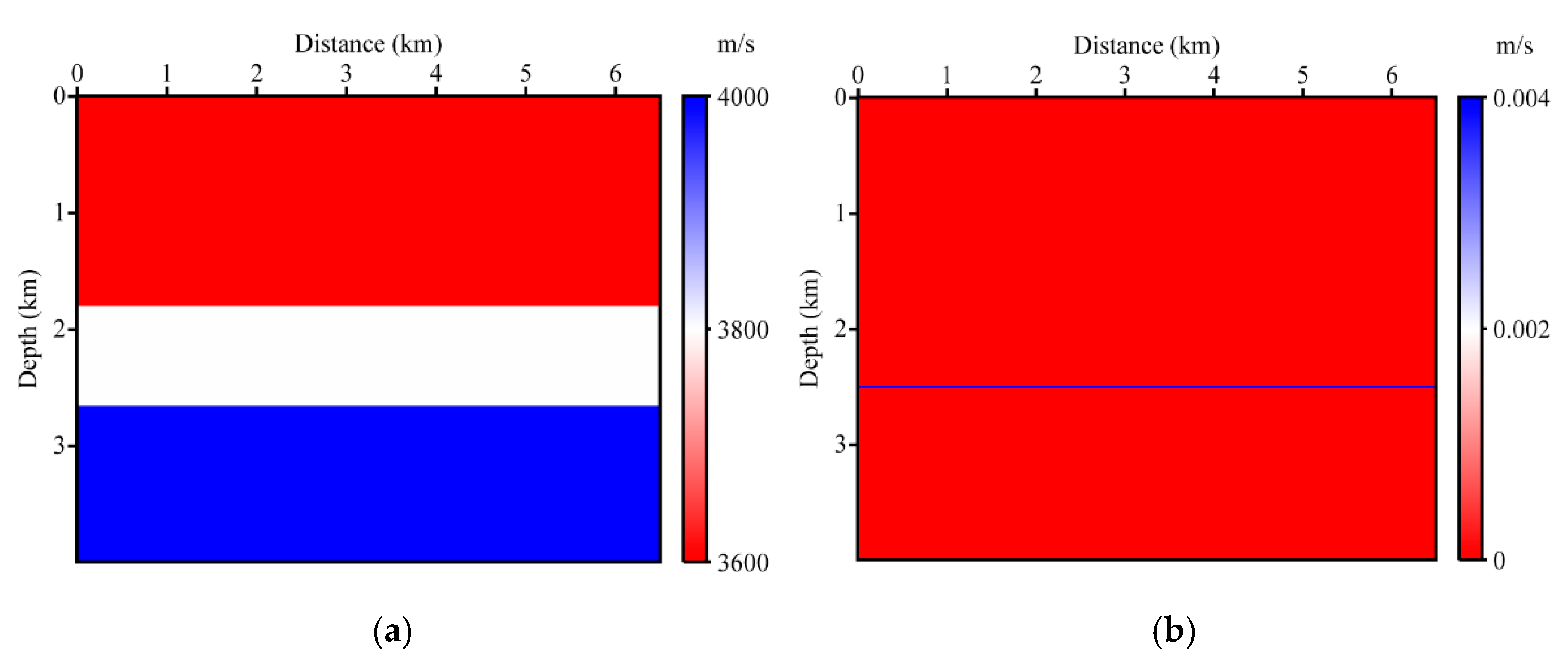
In the first example, we employ a layered velocity model to probe the performance of the above equations. The P-wave migration velocity model is sketched in Figure 1a. The S-wave migration velocity is obtained using an empirical formula . The density is set as 2000 kg/m3. The model is dispersed by 650 × 400 grid numbers, with a grid size of 10 × 10 m2. A Ricker wavelet with the dominant frequency of 25 Hz is set as the source signature at the location of (1 km, 0). The wavefields are simulated by the finite difference method with the second-order in time and tenth-order in space. In addition, we add a perfectly matched layer around the simulated area to absorb spurious reflections from the truncated boundary.
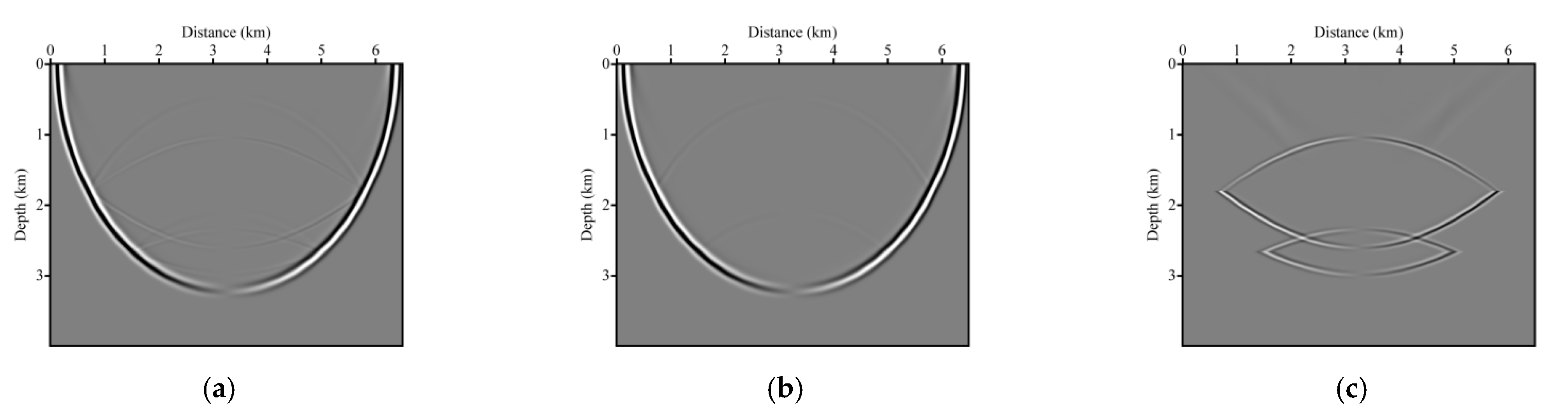
Based on the VCWE, the -component of the particle-velocity is shown in Figure 2a, in which the P- and S-waves are coupled together. When the coupled wavefield is extrapolated by solving Equation (4), it can be completely decoupled into pure P- and S-waves (Figure 2b,c). Notably, the seismic energy of the deep structure information is relatively weak in the decoupled wavefield.
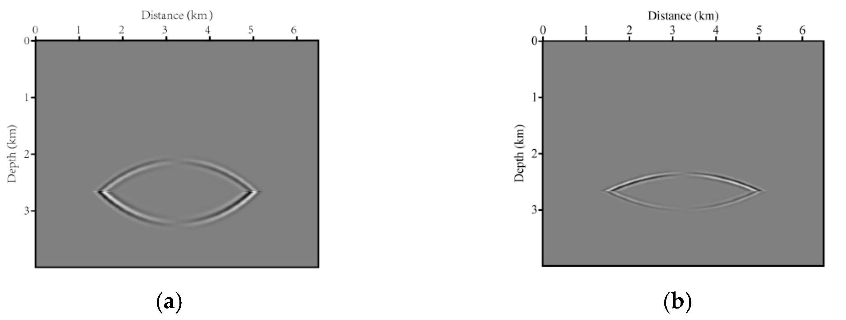
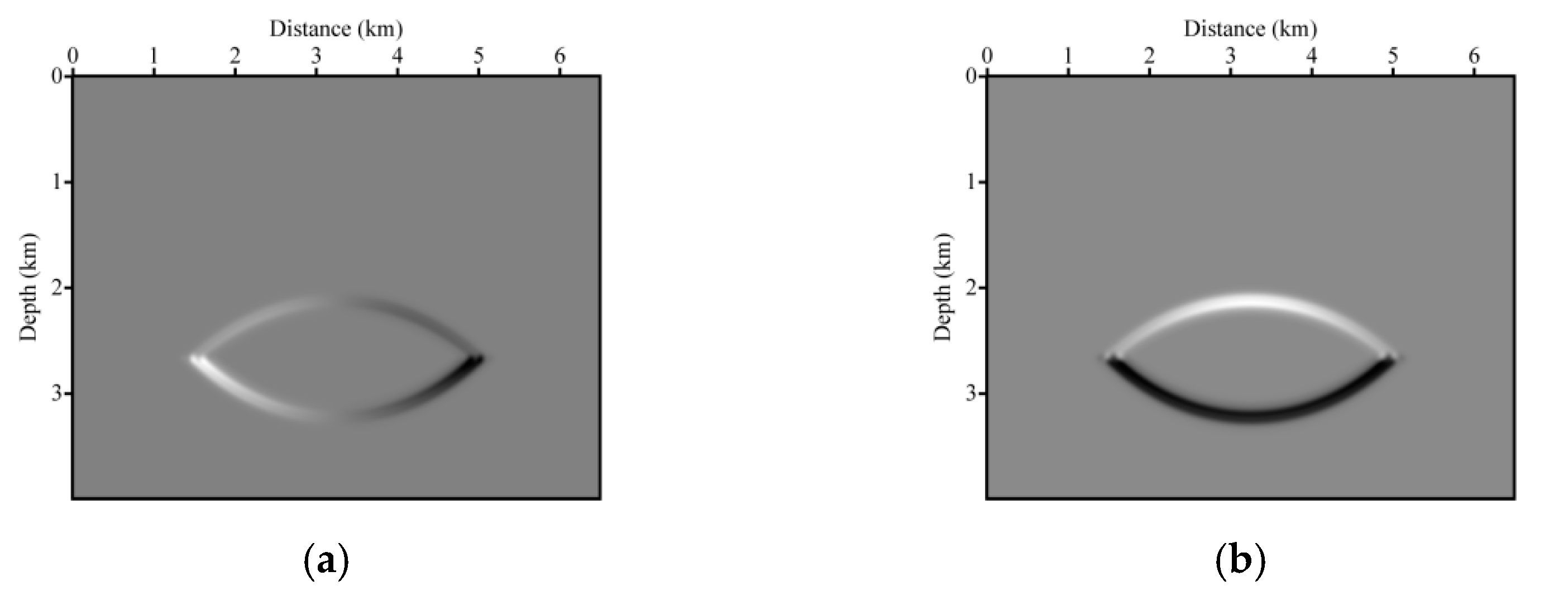
To reduce the shielding effect of the overburden rock on seismic waves, we simulate the wavefield based on SVDWE. Here, the second interface is set as the stained target. is obtained by multiplied 10−6 in the target area while is zero in other locations. The setting of is similar to that of . Considering the similarity between and models, only one of them is shown in Figure 1b. By solving SVDWE, the stained wavefield is generated after the hits the stained target. The stained wavefield only contains the reflection and transmission about the second interface as exhibited in Figure 3. Consequently, we infer that imaging with the stained wave can reduce interference from non-target structures.
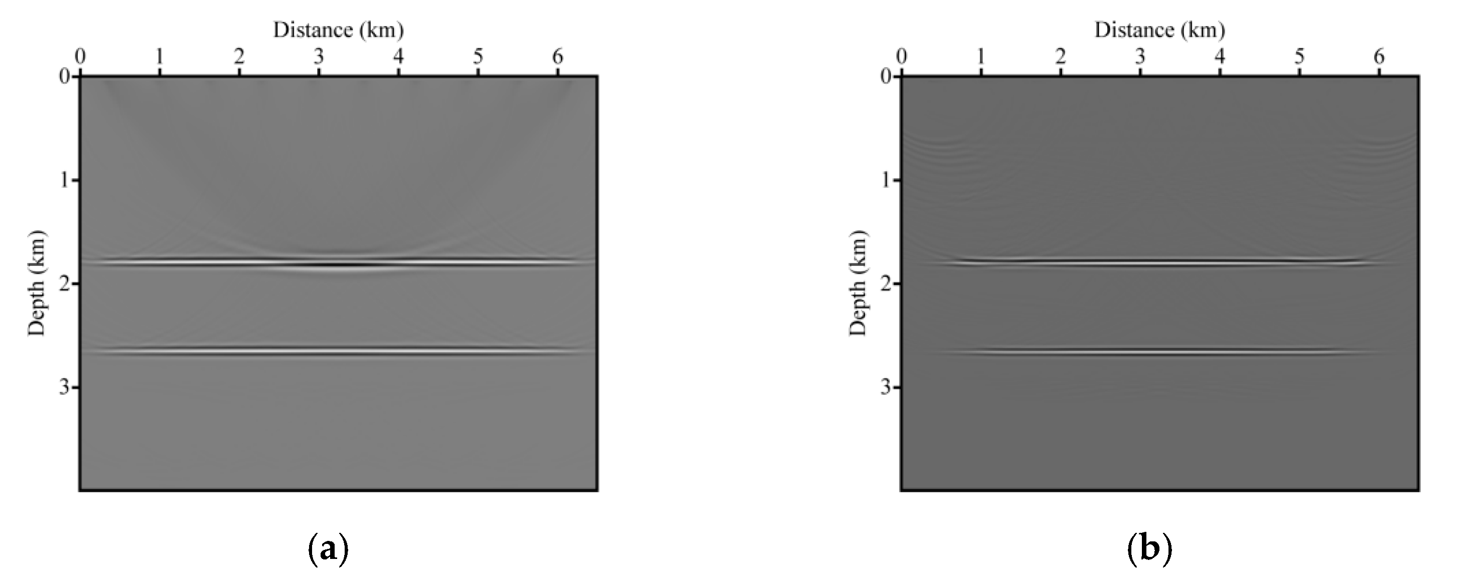
Furthermore, we utilize a contrastive approach to illustrate the adaptability of the ERTM for different equations. We evenly deploy 10 shots and 650 receivers on the surface of the layered velocity model. The total length of seismic records is 3 s, with a step time of 1ms. Figure 4 shows the multi-shot stacked images based on VDWE. Moreover, we implement the ERTM using the SVDWE, the PP and PS images are sketched in Figure 5. The settings of the stained target are the same as those of previous numerical experiments. Thanks to the stained wavefields, the primary information in the images is the second interface. However, some unwanted migration artifacts may interfere with subsequent interpretations.
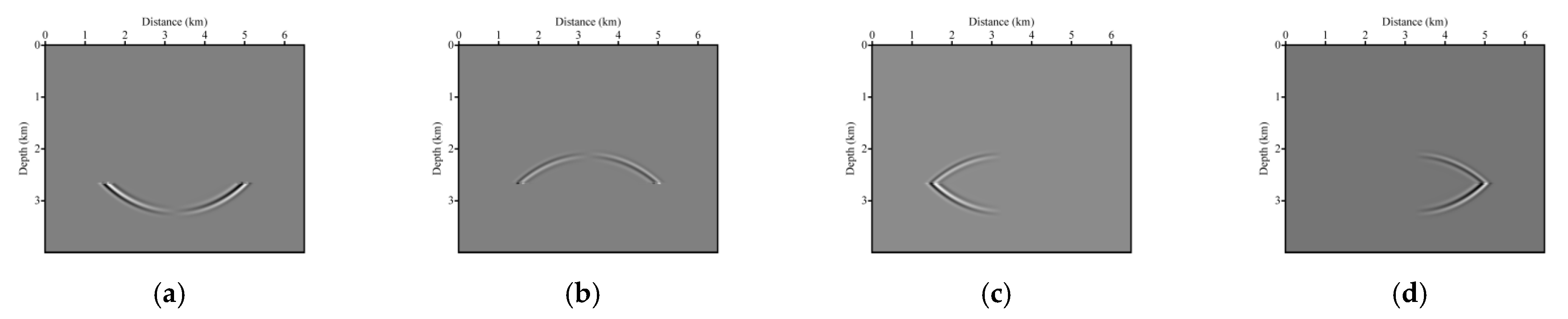
Next, we demonstrate that the proposed imaging condition plays an important role in eliminating migration artifacts. The filters in the imaging condition need to be prepared in advance, and their properties are determined by the direction vector and Poynting vector. For the snapshot shown in Figure 3a, the Poynting vector (Figure 6) can be obtained using Equation (15). Here, we exhibit four filtered wavefields (Figure 7) that, respectively, correspond to different direction vectors: , , , and .
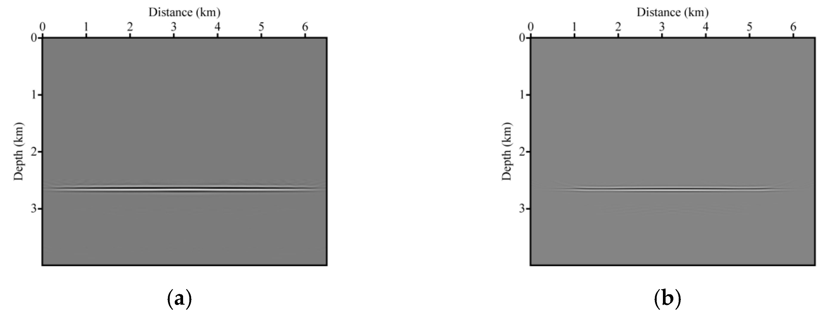
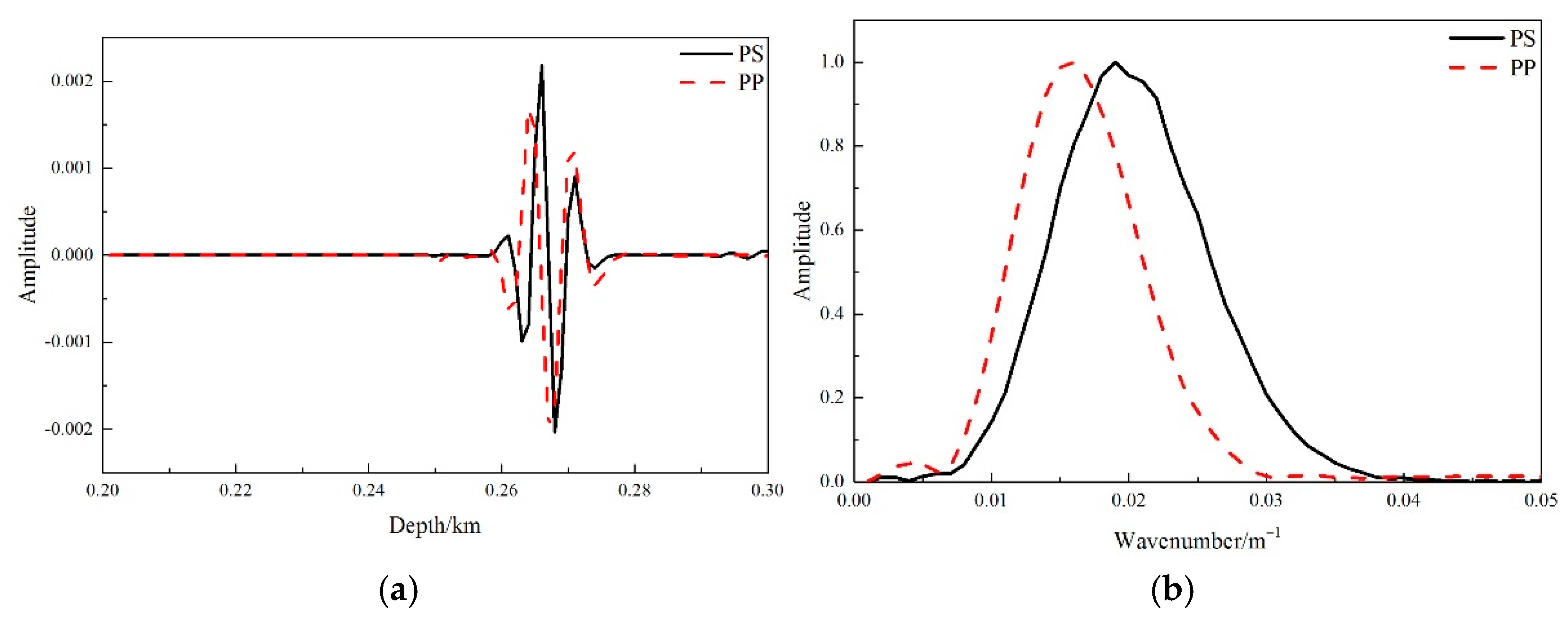
For flat strata, images with fewer artifacts can be obtained in the inner product of the up-going stained source wavefield and the down-going stained receiver wavefield (Figure 8). Figure 9 quantitatively compares PP and PS images, and the two sets of single-channel data are extracted from Figure 8 (from 2 km to 3 km in depth), and then mapped to the wavenumber domain through the Fourier transform. It is prominent that PS images are characterized by abundant high wavenumber information, robustly confirming that PS images have a higher spatial resolution than PP images. The basic reason for such a phenomenon is that S-wave travels slower than P-wave in the subsurface. Namely, the converted S-waves possess a shorter wavelength.
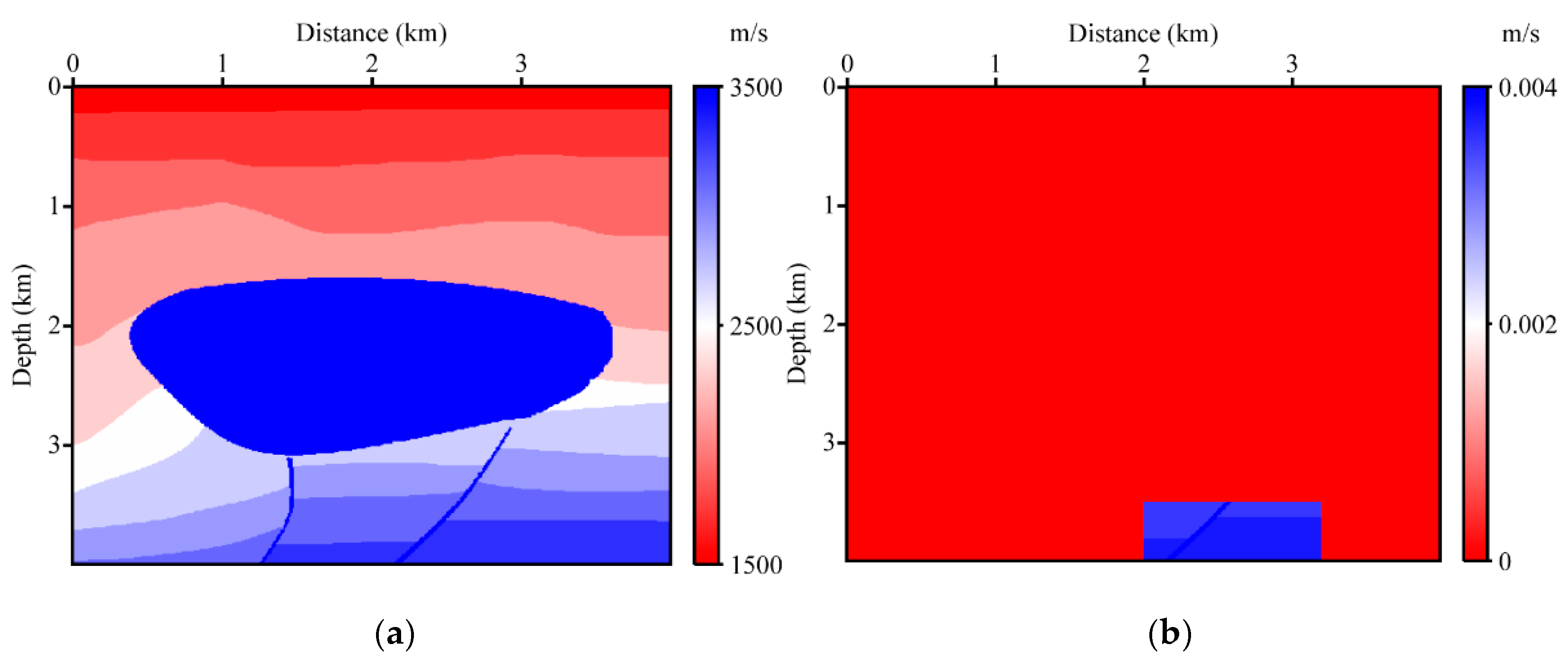
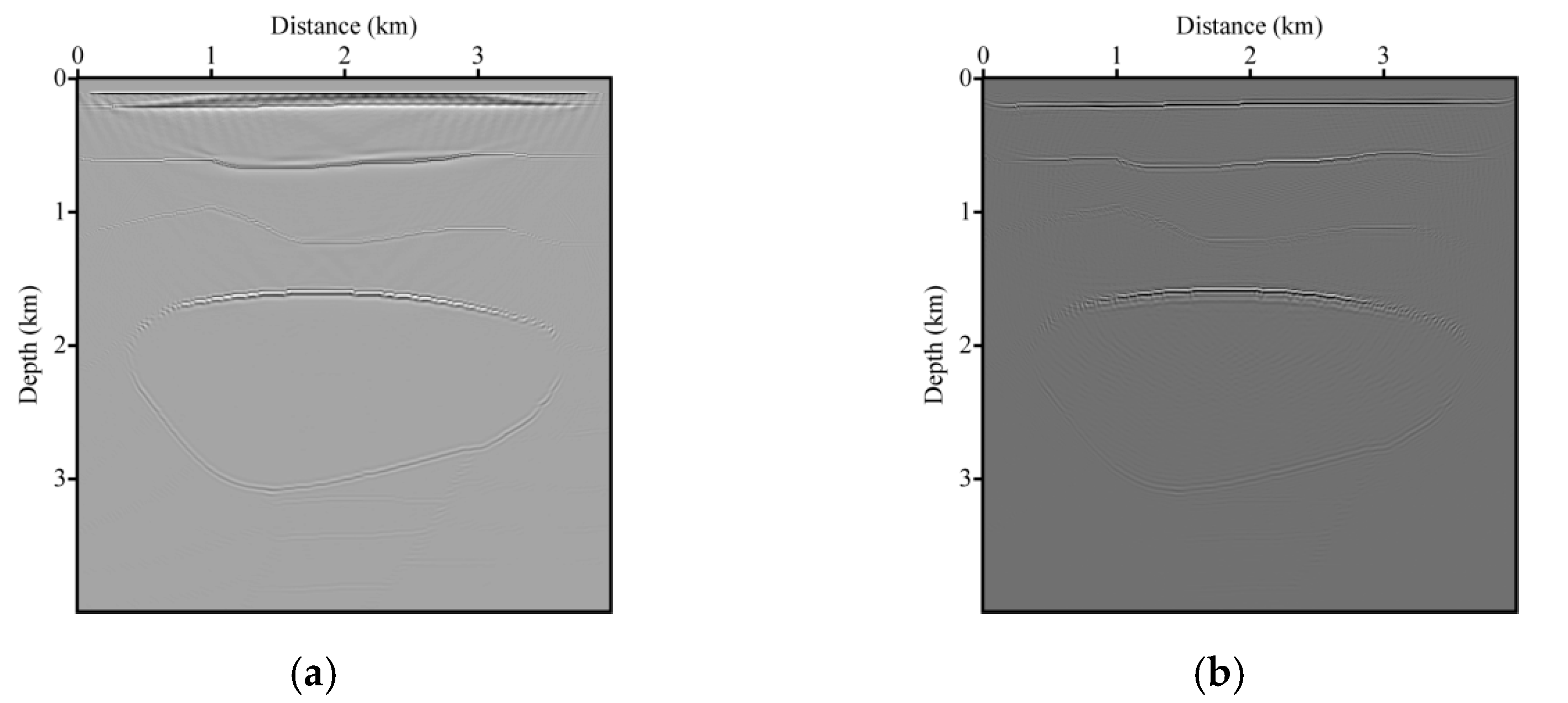
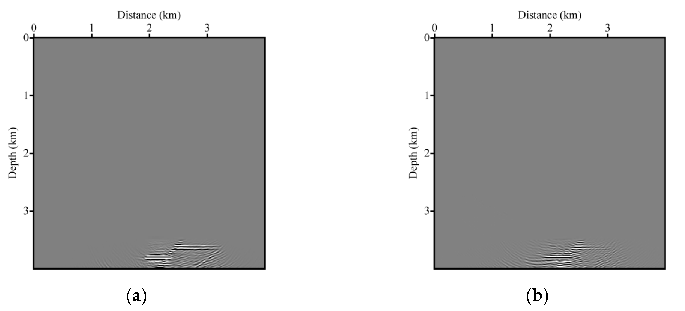
In this example, a salt model is applied to evaluate the efficiency of the proposed approach in complex geologic regions. The true P-wave velocity model is exhibited in Figure 10a, and S-wave velocity is also calculated using the previous empirical formula. The model size is 400 × 400 grids, with a grid size of 10 × 10 m2 in both horizontal and vertical directions. A total of 40 sources are evenly excited on the surface of the model. Each source has 400 receivers with a spacing of 10 m. The maximum recording time is 6 s. Figure 11 shows the PP and PS images obtained by the conventional ERTM, and it is obvious that the shallow structure and the salt boundary can be effectively identified. However, the high-velocity overburden rock leads to insufficient illumination for the deep subsurface, which ultimately blurs the subsalt image. We set the stained target in Figure 10b. Figure 12 displays the PP and PS images with the proposed imaging condition. We can see that the two complementary images are favorable for the identification of subsalt faults.
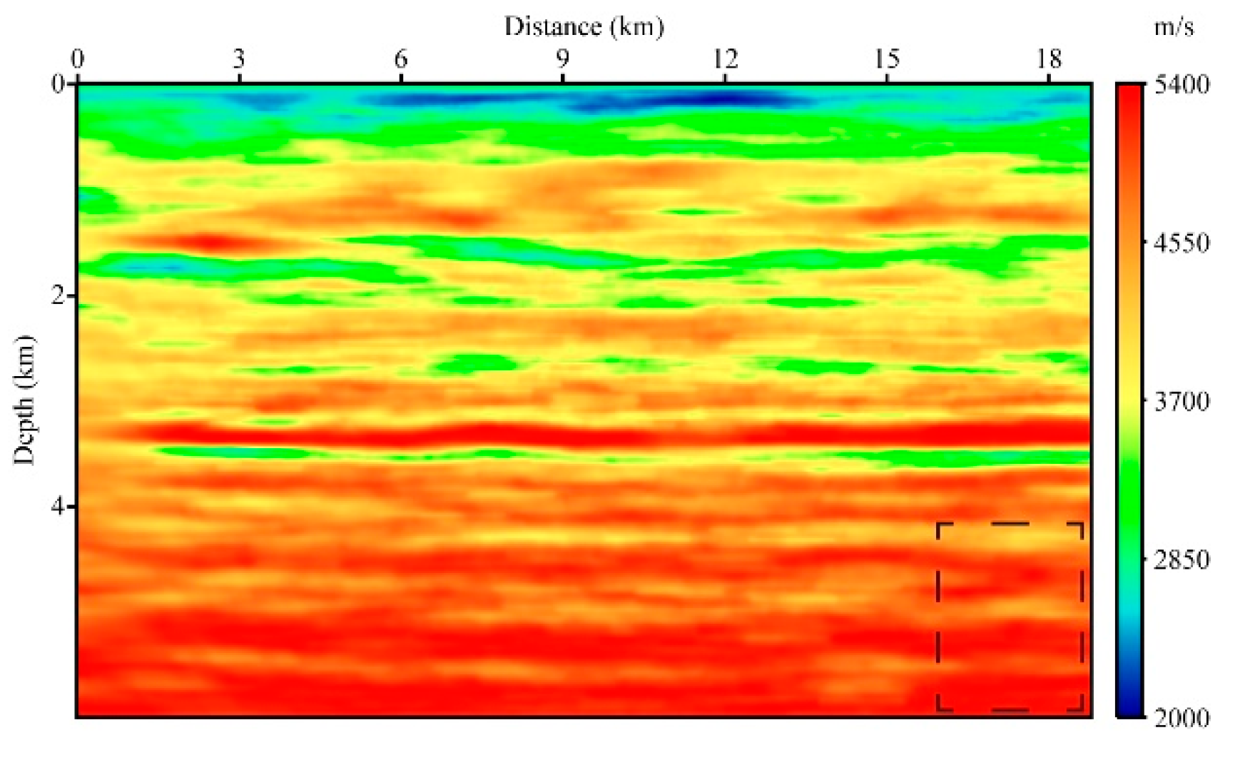
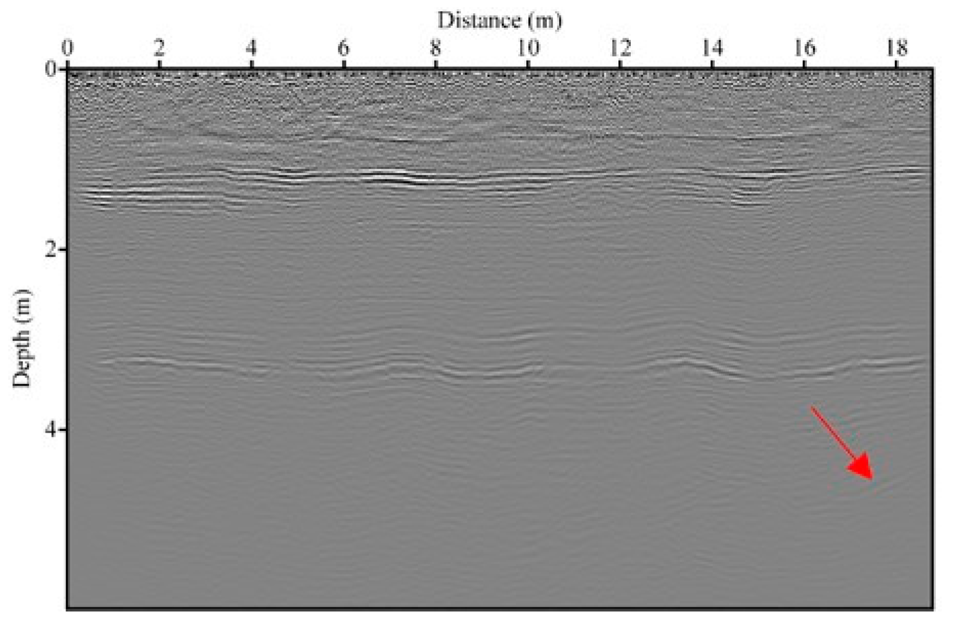
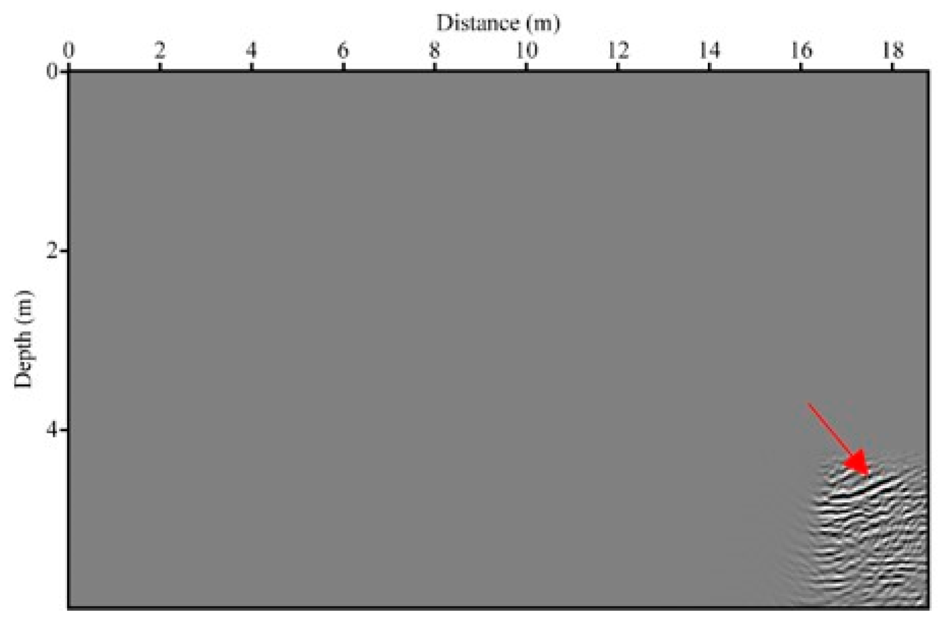
In the last experiment, a field data is utilized to confirm the effectiveness of our method. Figure 13 displays the migration velocity model that has 940 × 300 grid points with a 20 × 20 m2 element. There are 240 sources unevenly distributed at the free surface. Figure 14 show some shot gathers whose maximum recording time is 5 s. Since we only have the vertical component of the seismic record where P-wave information dominates, the valuable PS images are not obtained. The PP images based on VDWE are sketched in Figure 15, from which we can see the main structures. To enhance the quality of imaging in weakly illuminated areas, we set the box in Figure 13 as the stained targets. By using the proposed method, the migration events (Figure 16) relevant to the stained targets are highlighted, and the reflections of nontarget structures are muted.
4. Discussion
Our approach shows the satisfying performance for imaging weakly illuminated structures. When an overall migrated profile is acquired, it is proper to achieve locally enhanced imaging by artificially setting exploration targets in advance. Since the SVDWE contains two systems of equations, the algorithm of such an approach is twice as computationally intensive as the conventional one. The staining strategy is intrinsically related to the imaging results and is worthy of further investigation. The filters in the inner product imaging condition screen different wavefields according to the direction of wave propagation. Theoretically, it is possible to achieve wavefield decomposition in an arbitrary direction. However, in this paper, we decompose the wavefield into up- and down-going categories under the assumption that the target structure is relatively flat. To enhance the imaging adaptability for complex geological situations, the wavefield screening method according to stratigraphic dip angle needs to be persistently explored.
5. Conclusions
We have presented a new ERTM technique to produce the weakly illuminated structure. To extract the elastic wavefield related to the target, a stained vector-decoupled wave equation is adopted. The filter in the inner product imaging condition can suppress the migration artifact, improving the resolution of ERTM results. Numerical results show that our method can generate better amplitude for the weakly illuminated structure, providing possible technical support for reducing the risk of hydrocarbon development.
Author Contributions
Conceptualization, Y.S. and L.S.; methodology, Y.S.; software, W.L.; validation, Y.S. and L.S.; formal analysis, W.L.; investigation, L.S.; resources, Y.S.; data curation, Y.S.; writing—original draft preparation, L.S.; writing—review and editing, L.S.; visualization, W.L.; supervision, Y.S. and Q.Z.; project administration, Y.S. and Q.Z.; funding acquisition, Y.S. and L.S. All authors have read and agreed to the published version of the manuscript.
Funding
This research was funded by the National Natural Science Foundation of China (U19B6003-004), the National Key R&D Program of China (2018YFA0702505), the National Natural Science Foundation of China (41930431) and the University Nursing Program for Young Scholars with Creative Talents in Heilongjiang Province (Grant No. UNPYSCT-2020149).
Institutional Review Board Statement
Not applicable.
Informed Consent Statement
Not applicable.
Data Availability Statement
Not applicable.
Conflicts of Interest
The authors declare no conflict of interest.
References
- Baysal, E.; Dan, D.K.; Sherwood, J. Reverse-Time Migration. Geophysics 1983, 48, 1514–1524. [Google Scholar] [CrossRef] [Green Version]
- McMechan, G. Migration by extrapolation of time-dependent boundary values. Geophys. Prospect. 1983, 31, 413–420. [Google Scholar] [CrossRef]
- Leveille, J.P.; Jones, I.F.; Zhou, Z.Z.; Wang, B.; Liu, F.Q. Subsalt imaging for exploration, production, and development: A review. Geophysics 2011, 76, WB3–WB20. [Google Scholar] [CrossRef]
- Liu, Y.; Chang, X.; Jin, D.; He, R.; Sun, H.; Zheng, Y. Reverse time migration of multiples for subsalt imaging. Geophysics 2011, 76, WB209–WB216. [Google Scholar] [CrossRef]
- Vigh, D.; Kapoor, J.; Moldoveanu, N.; Li, H. Breakthrough acquisition and technologies for subsalt imaging. Geophysics 2011, 76, WB41–WB51. [Google Scholar] [CrossRef]
- Regone, C. Using 3D finite-difference modeling to design wide-azimuth surveys for improved subsalt imaging. In Proceedings of the 2006 SEG International Exposition and Annual Meeting, New Orleans, LA, USA, 1–6 October 2006. [Google Scholar]
- Gherasim, M.; Albertin, U.; Nolte, B.; Askim, O.; Trout, M.; Hartman, K. Wave-equation angle-based illumination weighting for optimized subsalt imaging. In Proceedings of the 2010 SEG International Exposition and Annual Meeting, Denver, CO, USA, 17–22 October 2010. [Google Scholar]
- Cao, J.; Wu, R. Fast acquisition aperture correction in prestack depth migration using beamlet decomposition. Geophysics 2009, 74, S67–S74. [Google Scholar] [CrossRef]
- Chen, B.; Jia, X. Staining algorithm for seismic modeling and migration. Geophysics 2014, 79, S121–S129. [Google Scholar] [CrossRef] [Green Version]
- Li, Q.; Jia, X. Generalized staining algorithm for seismic modeling and migration. Geophysics 2017, 82, T17–T26. [Google Scholar] [CrossRef]
- Song, L.; Shi, Y.; Chen, S. Target-oriented reverse time migration in transverse isotropy media. Acta Geophys. 2021, 69, 125–134. [Google Scholar] [CrossRef]
- Sun, R.; McMechan, G.; Lee, C.; Chow, J.; Chen, C. Prestack scalar reverse-time depth migration of 3D elastic seismic data. Geophysics 2006, 71, S199–S207. [Google Scholar] [CrossRef]
- Yan, J.; Sava, P. Isotropic angle-domain elastic reverse-time migration. Geophysics 2008, 73, 229–239. [Google Scholar] [CrossRef] [Green Version]
- Du, Q.; Zhu, Y.; Ba, J. Polarity reversal correction for elastic reverse time migration. Geophysics 2012, 77, S31–S41. [Google Scholar] [CrossRef]
- Li, Z.; Ma, X.; Fu, C.; Liang, G. Wavefield separation and polarity reversal correction in elastic reverse time migration. J. Appl. Geophys. 2016, 127, 56–67. [Google Scholar] [CrossRef]
- Zhang, W.; Shi, Y. Imaging conditions for elastic reverse time migration. Geophysics 2019, 84, S95–S111. [Google Scholar] [CrossRef]
- Zhang, Y.; Sun, J. Practical issues in reverse time migration: True amplitude gathers, noise removal and harmonic source encoding. First Break 2009, 27, 53–59. [Google Scholar] [CrossRef]
- Sava, P.C.; Fomel, S. Angle-domain common-image gathers by wavefield continuation methods. Geophysics 2003, 68, 1065–1074. [Google Scholar] [CrossRef]
- Liu, Q.; Zhang, J. Efficient dip-angle adcig estimation using poynting vector in acoustic RTM and its application in noise suppression. Geophys. Prospect. 2018, 66, 1714–1725. [Google Scholar] [CrossRef] [Green Version]
- Liu, F.; Zhang, G.; Morton, S.A.; Leveille, J.P. An effective imaging condition for reverse-time migration using wavefield decomposition. Geophysics 2011, 76, S29–S39. [Google Scholar] [CrossRef]
- Fei, T.; Luo, Y.; Yang, J.; Liu, H.; Qin, F. Removing false images in reverse time migration: The concept of de-primary. Geophysics 2015, 80, S237–S244. [Google Scholar] [CrossRef]
- Wang, Y.; Zheng, Y.; Xue, Q.; Chang, X.; Tong, F.; Luo, Y. Reverse time migration with Hilbert transform based full wavefield decomposition. Chin. J. Geophys. 2016, 59, 4200–4211. [Google Scholar]
- Guo, X.; Shi, Y.; Wang, W.; Jing, H.; Zhang, Z. Wavefield decomposition in arbitrary direction and an imaging condition based on stratigraphic dip. Geophysics 2020, 85, S299–S312. [Google Scholar] [CrossRef]
- Wang, W.; McMechan, G. Vector-based elastic reverse time migration. Geophysics 2015, 80, 245–258. [Google Scholar] [CrossRef] [Green Version]
- Lu, Y.; Liu, Q.; Zhang, J.; Yang, K.; Sun, H. Poynting and polarization vectors based wavefield decomposition and their application on elastic reverse time migration in 2D transversely isotropic media. Geophys. Prospect. 2019, 67, 1296–1311. [Google Scholar] [CrossRef]
Figure 1.
Migration model: (a) P-wave velocity; (b) Stained target.

Figure 2.
-component of particle-velocity wavefield: (a) Coupled wave; (b) Pure P-wave; (c) Pure S-wave.
Figure 2.
-component of particle-velocity wavefield: (a) Coupled wave; (b) Pure P-wave; (c) Pure S-wave.

Figure 3.
-component of the stained wavefield: (a) Pure P-wave; (b) Pure S-wave.

Figure 4.
ERTM image obtained based on the VDWE: (a) PP imaging; (b) PS imaging.

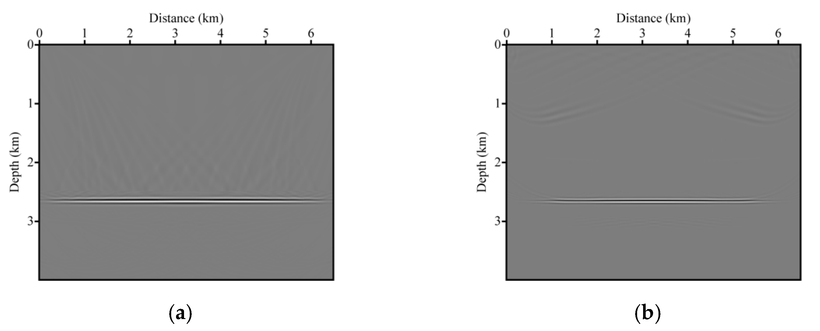
Figure 5.
ERTM image based on the SVDWE: (a) PP imaging; (b) PS imaging.

Figure 6.
Poynting vector: (a) -component; (b) -component.

Figure 7.
Filtered wavefield: (a) downgoing; (b) upgoing; (c) Leftgoing; (d) rightgoing.

Figure 8.
ERTM profile with fewer artifacts compared with Figure 5: (a) PP imaging; (b) PS imaging.
Figure 8.
ERTM profile with fewer artifacts compared with Figure 5: (a) PP imaging; (b) PS imaging.

Figure 9.
Comparison between PP and PS images: (a) Single-channel data; (b) Wavenumber spectrum.

Figure 10.
Migration model: (a) True P-wave velocity; (b) Stained target.

Figure 11.
ERTM images based on the VDWE: (a) PP imaging; (b) PS imaging.

Figure 12.
ERTM images based on the SVDWE: (a) PP imaging; (b) PS imaging.

Figure 13.
P-wave velocity.

Figure 14.
Two shot gathers.

Figure 15.
PP imaging based on VDWE.

Figure 16.
PP imaging based on SVDWE.

Publisher’s Note: MDPI stays neutral with regard to jurisdictional claims in published maps and institutional affiliations. |
© 2022 by the authors. Licensee MDPI, Basel, Switzerland. This article is an open access article distributed under the terms and conditions of the Creative Commons Attribution (CC BY) license (https://creativecommons.org/licenses/by/4.0/).
Share and Cite
MDPI and ACS Style
Song, L.; Shi, Y.; Liu, W.; Zhao, Q. Elastic Reverse Time Migration for Weakly Illuminated Structure. Appl. Sci. 2022, 12, 5264. https://0-doi-org.brum.beds.ac.uk/10.3390/app12105264
AMA Style
Song L, Shi Y, Liu W, Zhao Q. Elastic Reverse Time Migration for Weakly Illuminated Structure. Applied Sciences. 2022; 12(10):5264. https://0-doi-org.brum.beds.ac.uk/10.3390/app12105264
Chicago/Turabian StyleSong, Liwei, Ying Shi, Wei Liu, and Qiang Zhao. 2022. "Elastic Reverse Time Migration for Weakly Illuminated Structure" Applied Sciences 12, no. 10: 5264. https://0-doi-org.brum.beds.ac.uk/10.3390/app12105264
Note that from the first issue of 2016, this journal uses article numbers instead of page numbers. See further details here.