
XG Boost Algorithm to Simultaneous Prediction of Rock Fragmentation and Induced Ground Vibration Using Unique Blast Data

 ,
,
Abstract
:1. Introduction
Objectives
2. Materials and Methods
2.1. Predictability and Assessment of Blast Results
2.2. A Brief of the Mine and Blast Site
- a.
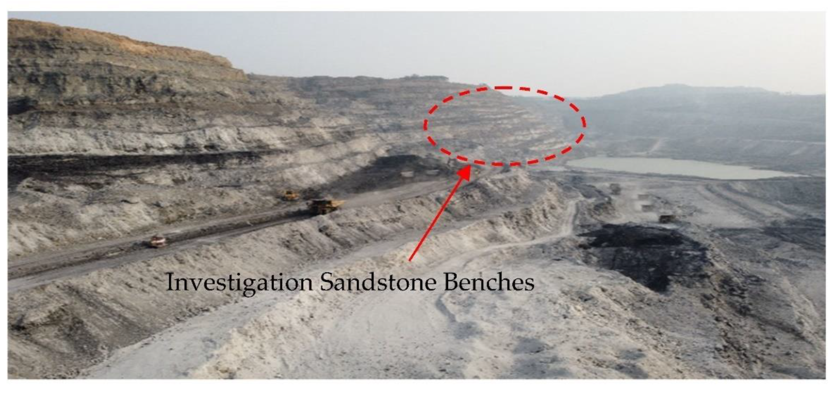
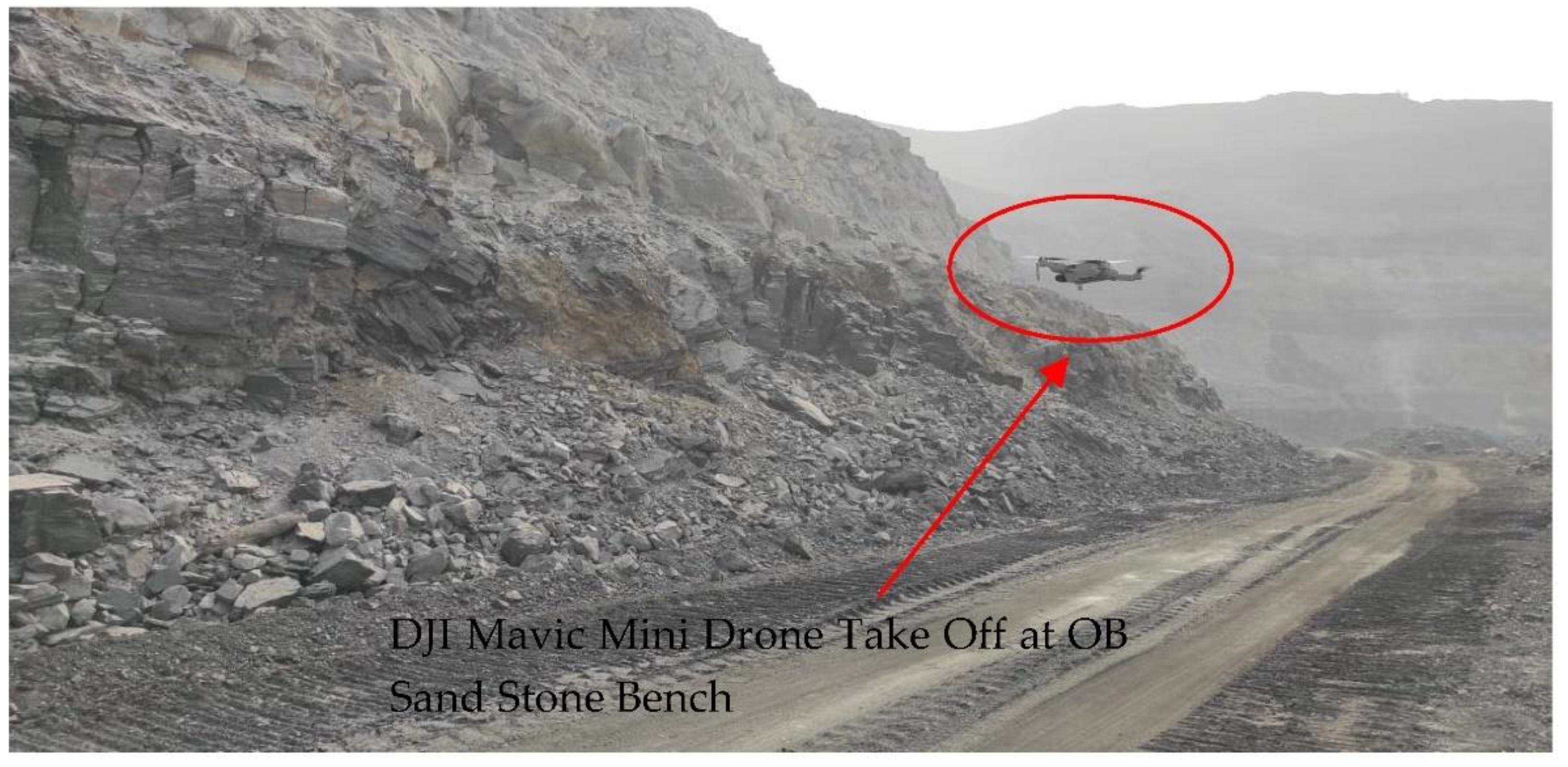
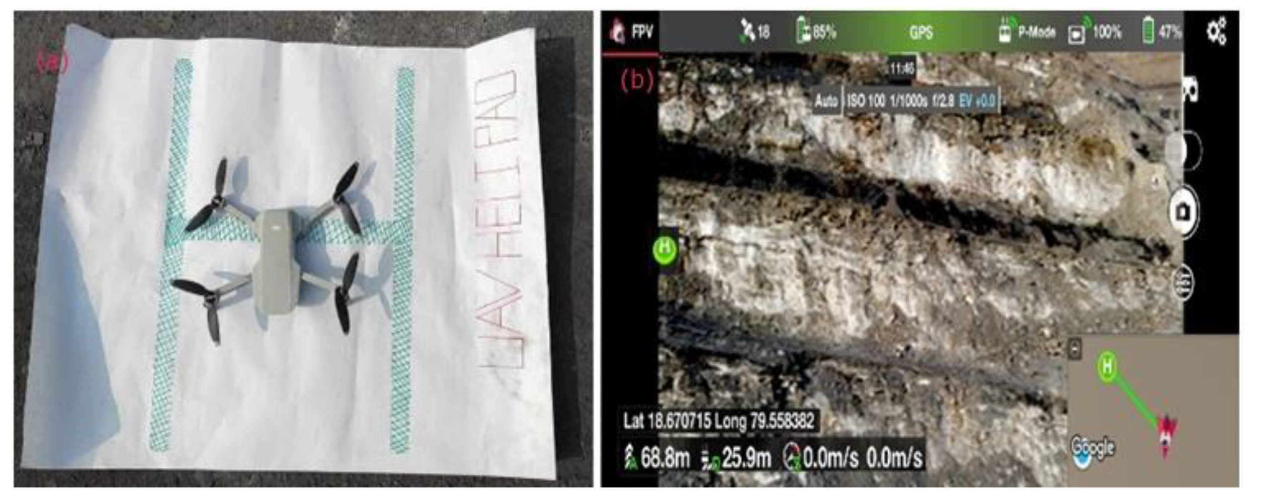
- Identification of bench structural geo-property through UAV:
- b.
- Geo–technical properties of the site:
2.3. AI Tools for Rock Characterization
2.4. Blast Modeling Using Software
2.5. Blast Experimentation
- 1.
- The four OB benches chosen for experimentation were 1 de-coaled, 3A coal seam, and 3A de-coaled with bench heights of 12 m, 10.5 m, 11 m, and 9.5 m, respectively. Because the mine was previously worked underground, there was a high risk of disturbances in strata and induction of cracks. To address this issue, benches were initially cleaned to a depth of 0.3 m for improved visibility and identification of cracks and joint planes, as shown in Figure 9a,b.

- 2.
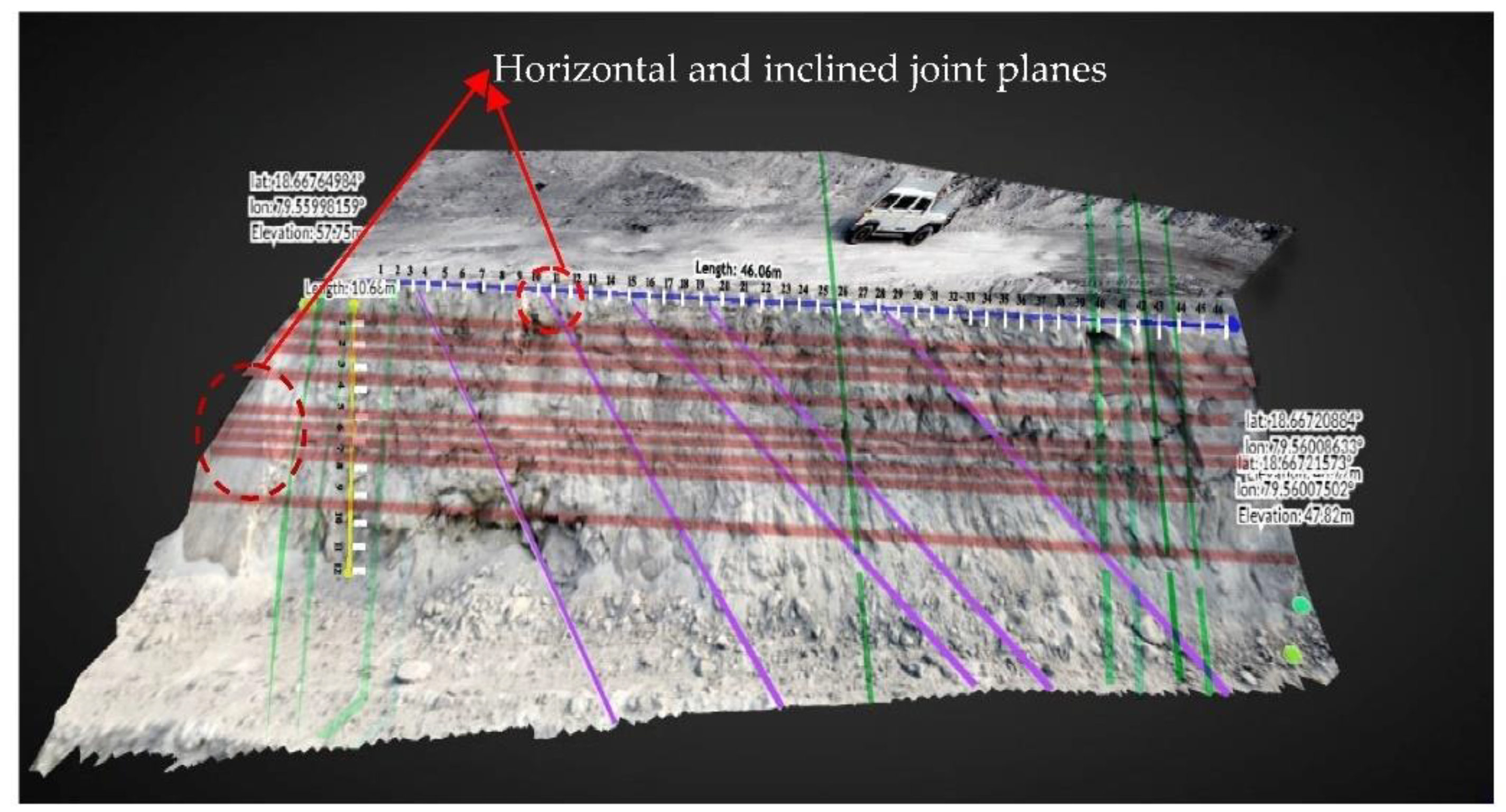
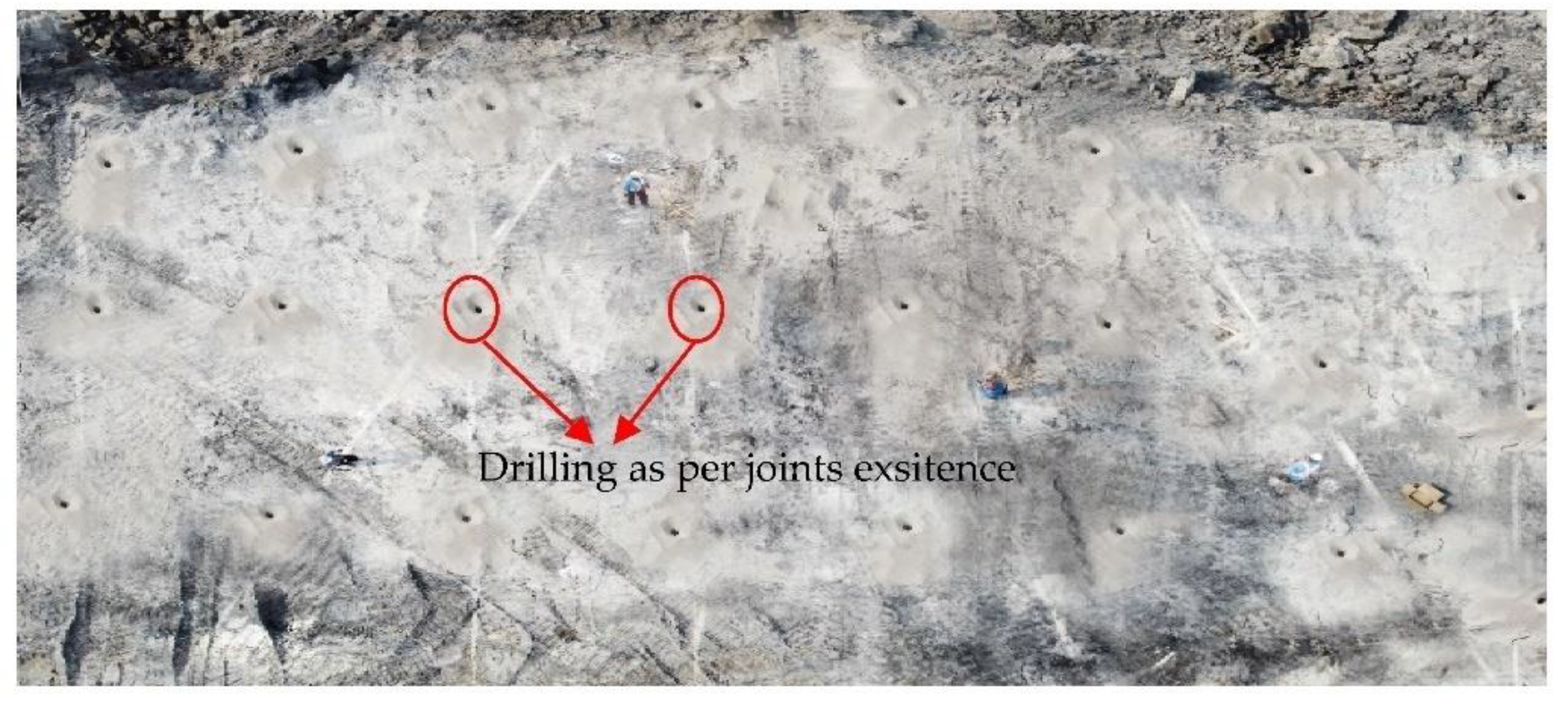
- The joint planes of the benches were identified by STRAYOS software and marked with white powder on the bench top surface to avoid the seizing-up of drilling bits in joints and to have a reference in deciding blast pattern and connections, as shown in Figure 10. Table 1 shows the design burden and spacing values in the O-PITBLAST that yielded good predicted results. The drill bit diameter was 150 mm, which was adequate for the existing bench height, burden, and spacing, and the drilled holes are shown in Figure 11.


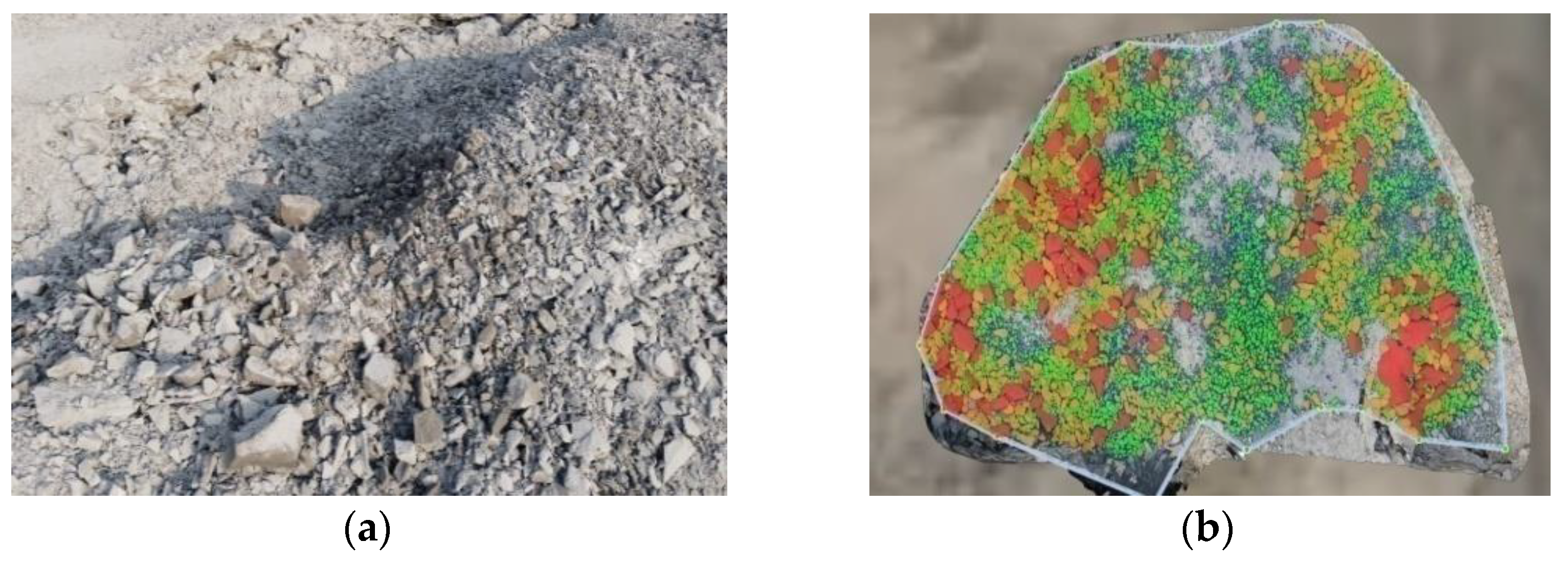
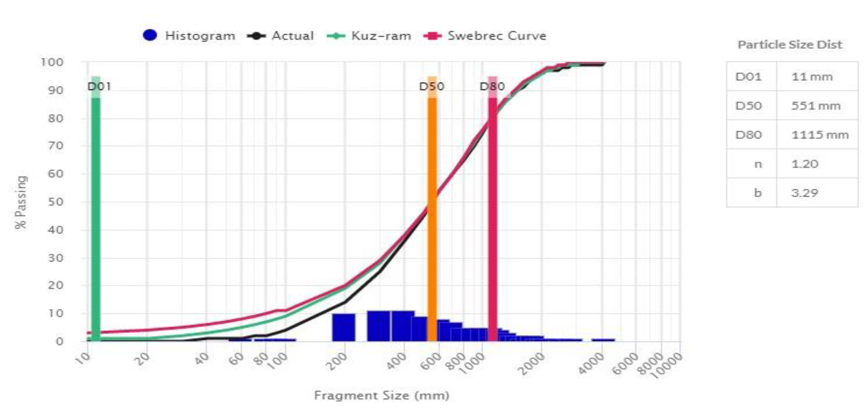
2.6. Assessment of Fragmentation
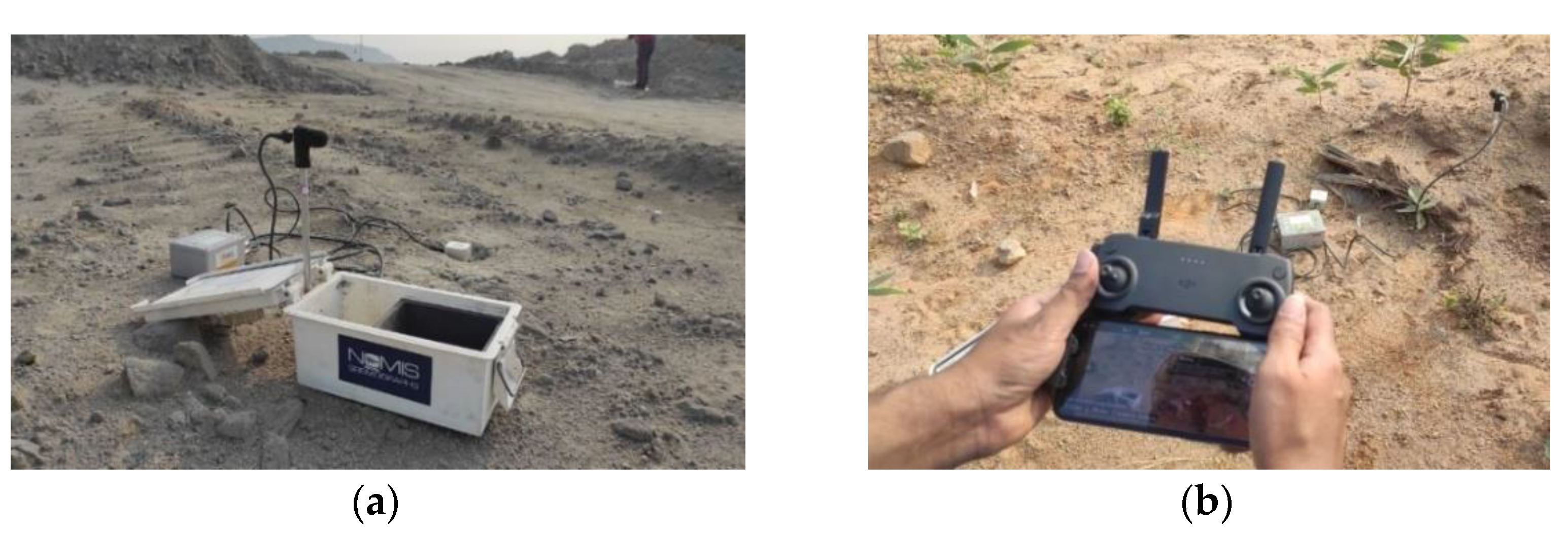
2.7. Ground Vibration
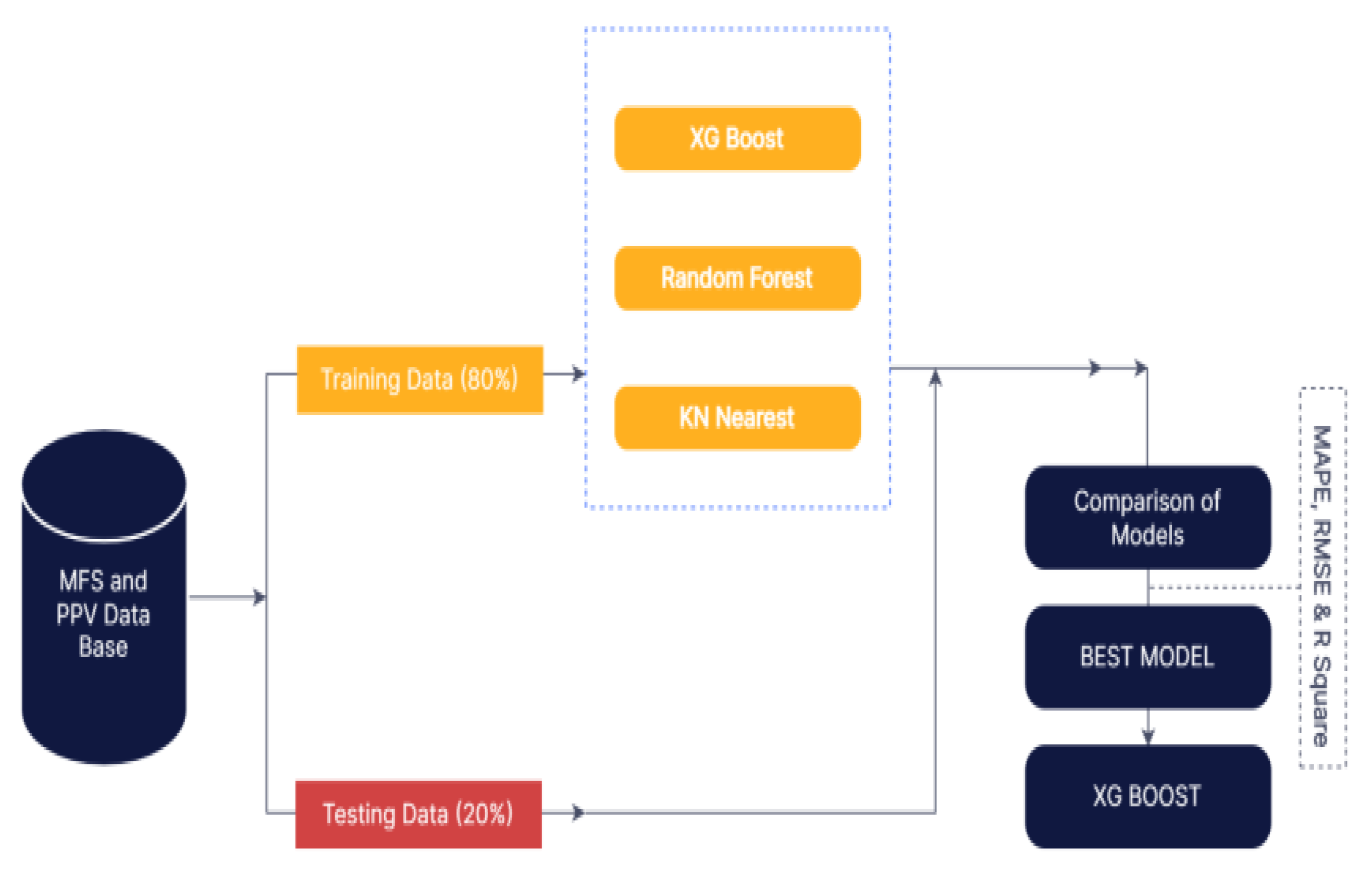
2.8. XG Boost Regression Algorithm
2.9. Random Forest Algorithm
- Based on the dataset, generate bootstrap samples that are the number of trees in the forest (ntree).
- Create an unpruned regression tree for each bootstrap sample by picking predictors at random (mtry). Choose the optimal split among those factors.
- Assemble the anticipated values of the trees to forecast fresh observations (ntree). The average value of the projected values by each tree in the forest was utilized to solve the regression problem as well as forecast fragmentation and blast-induced PPV.
K-NN Algorithm
3. Results and Discussions
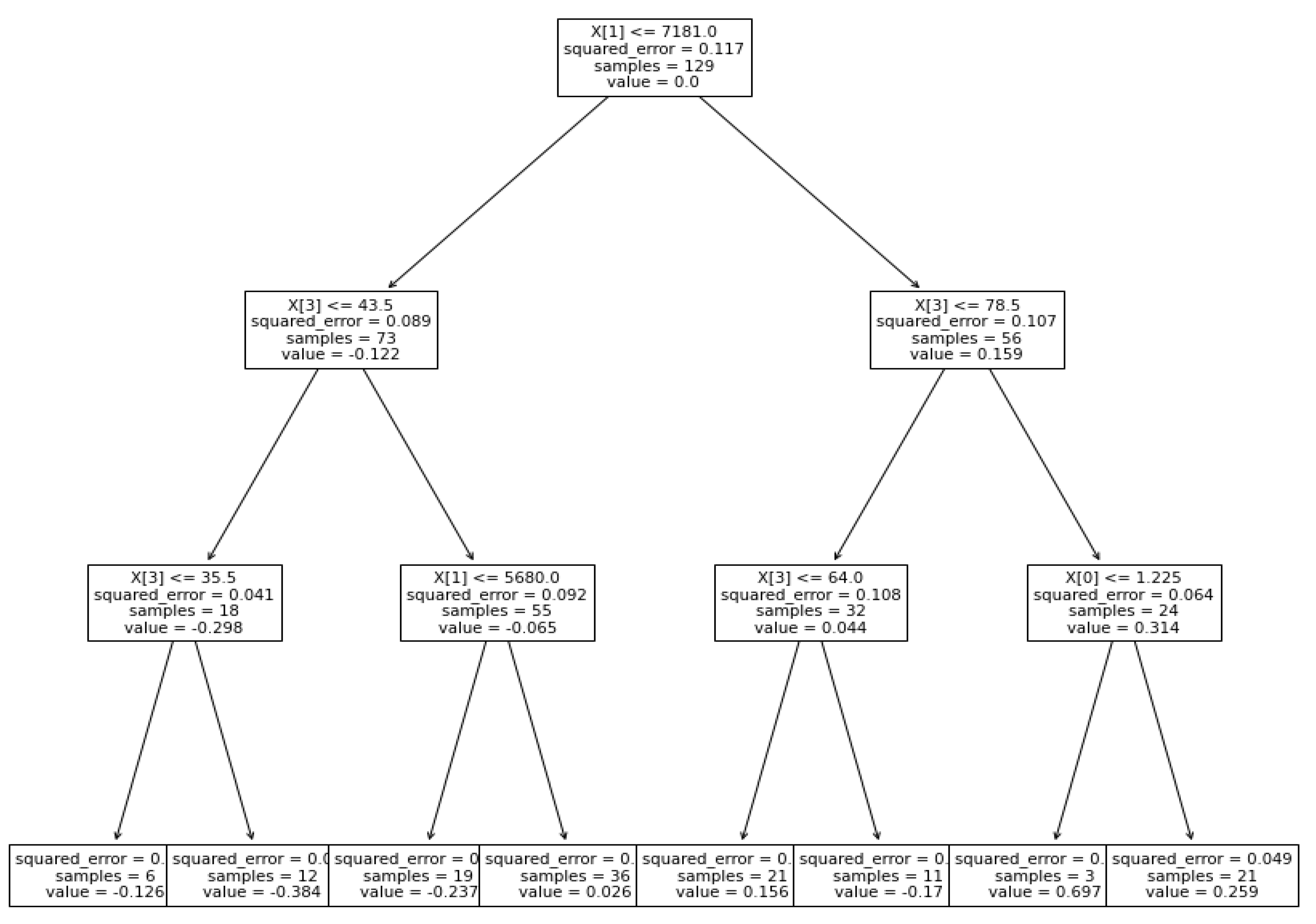
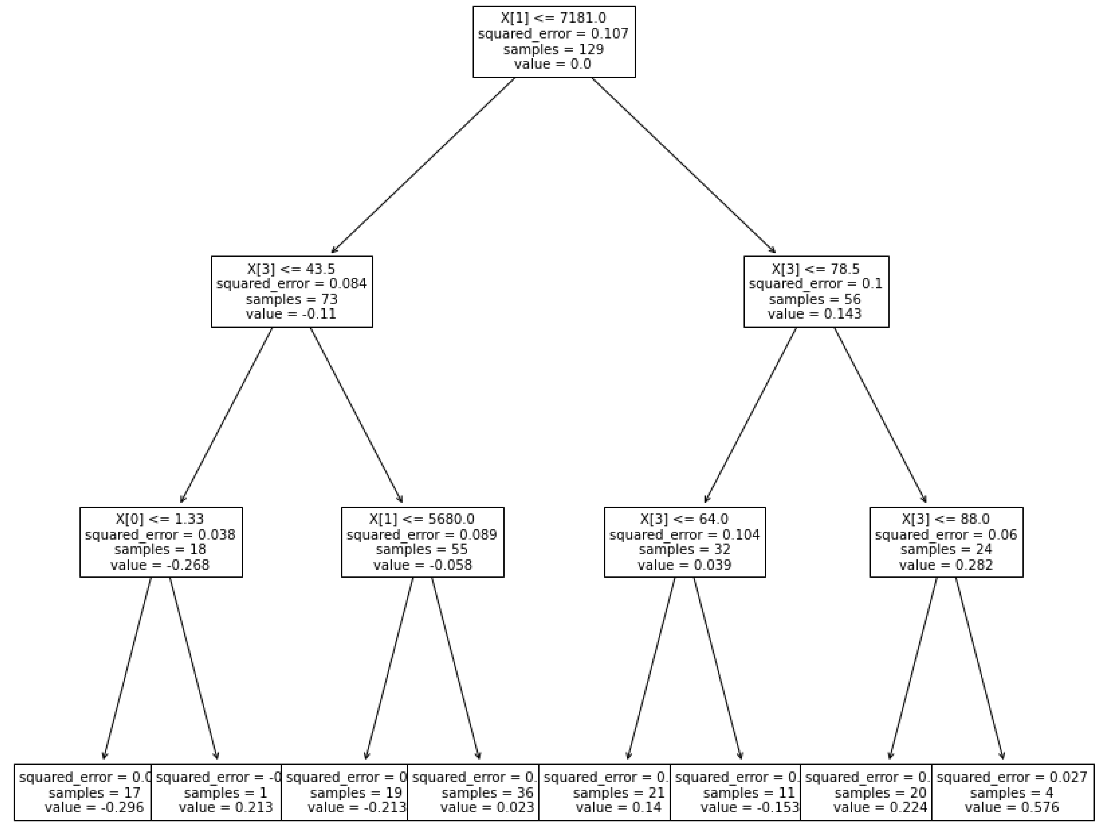
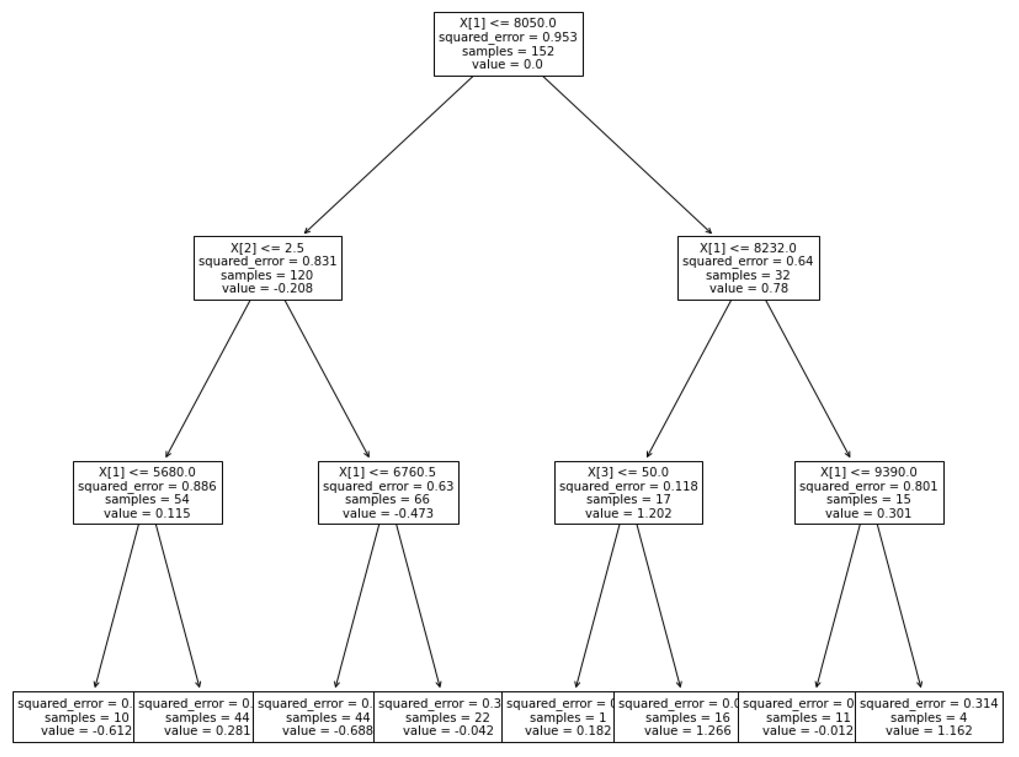
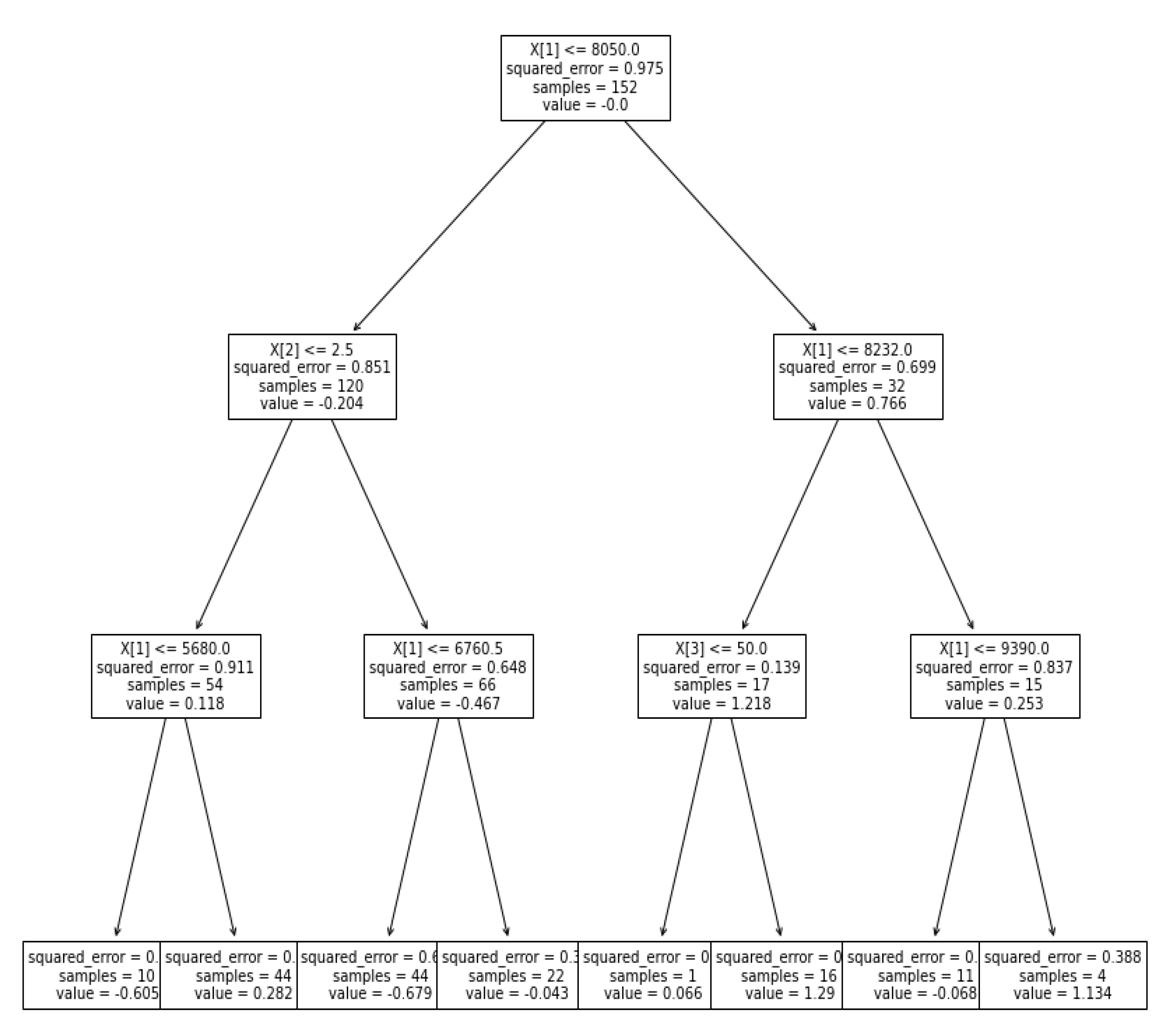
XG Boost Regression
4. Conclusions
- Use of O-PITBLAST SOFTWARE aided in the design of blasting and provided preliminary warnings for iterations.
- Available technical tools such as STRAYOS SOFTWARE are helpful in identifying the joint angle for rock mass characterization as well as fragmentation analysis
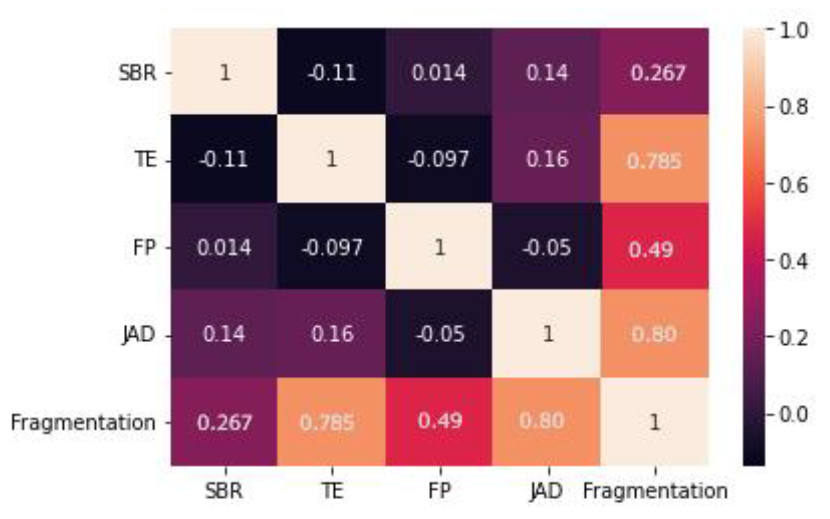
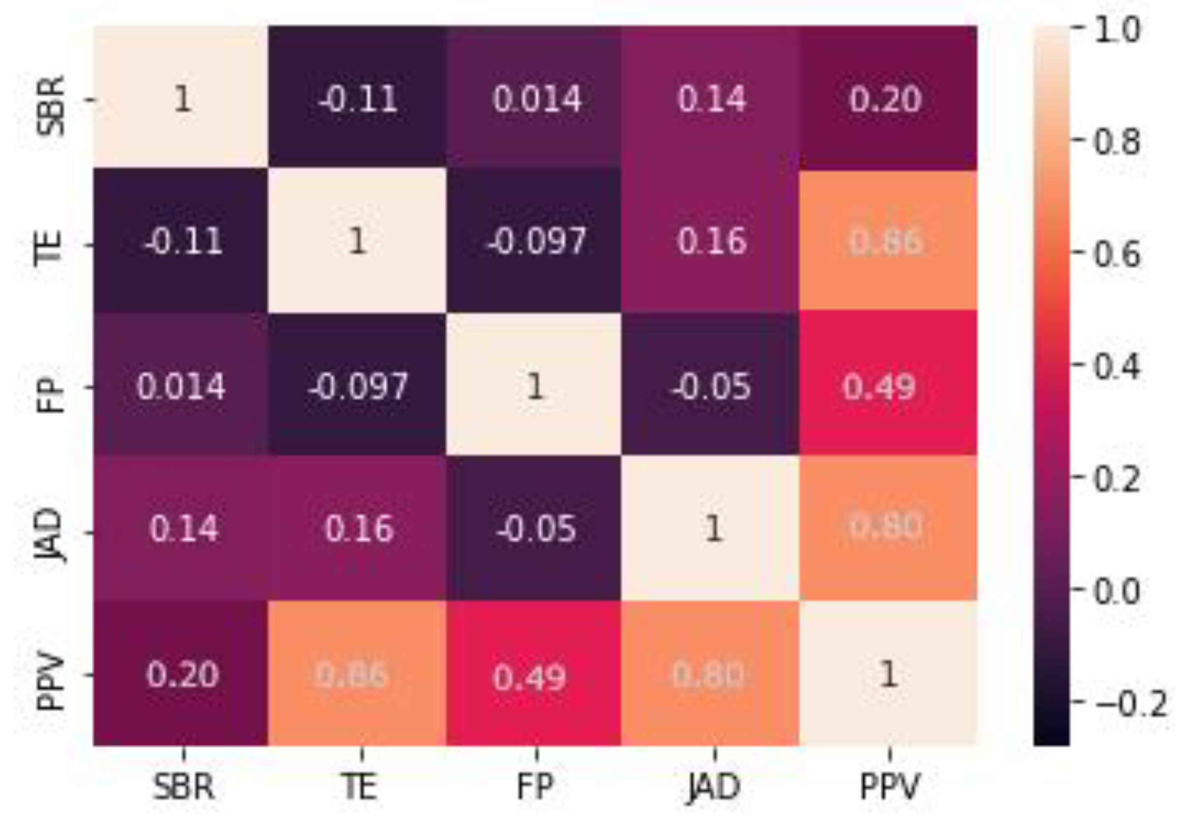
- A Correlation matrix was used to understand relationships between dependent and independent variables, and it proved to be quite useful.
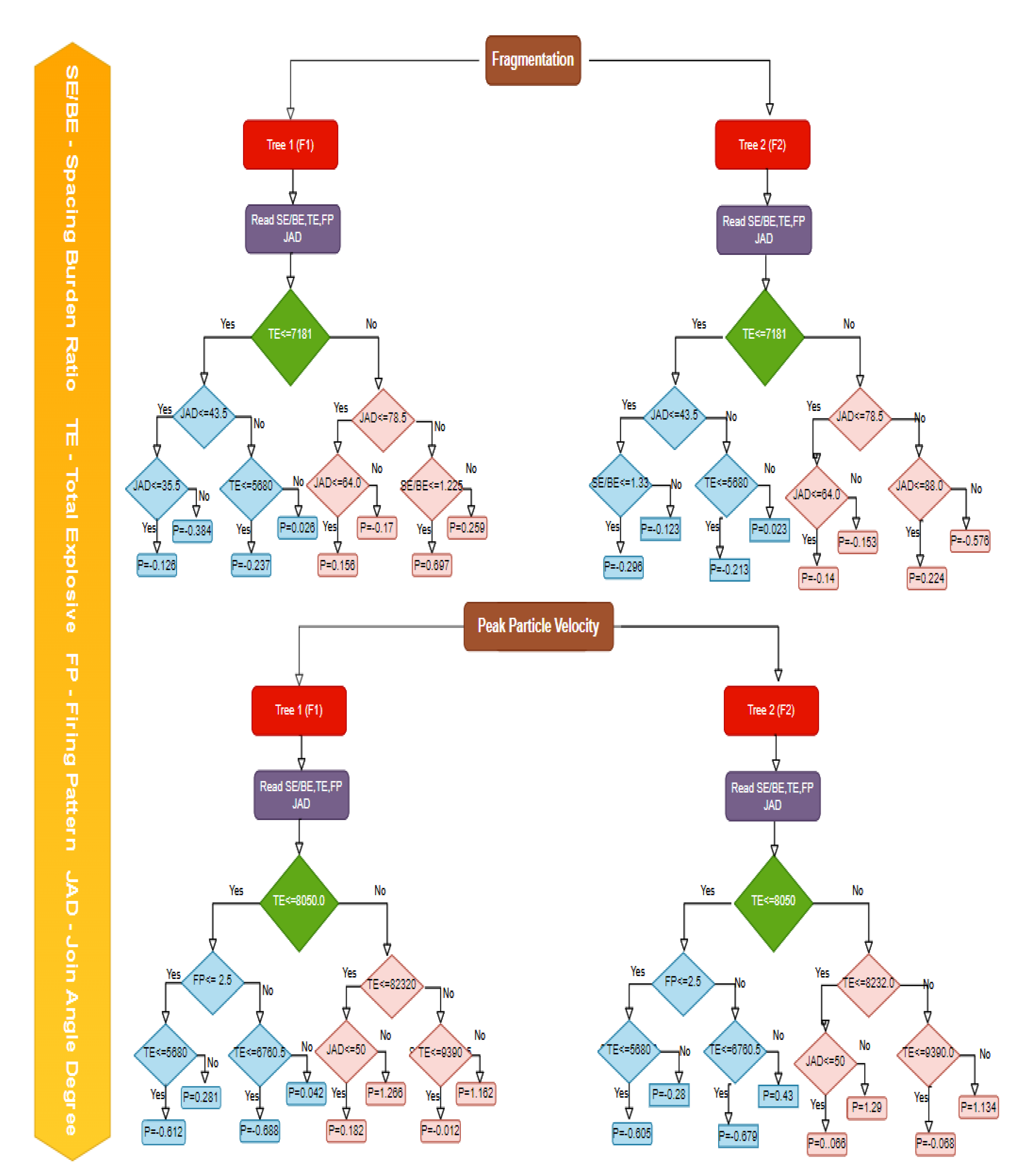
- The XG Boost Regression Algorithm was found to be useful for creating an empirical formula to forecast simultaneous fragmentation and peak particle velocity utilizing joint angle and other blast design parameters such as Se/Be ratio, Total Explosive, and Firing Pattern while keeping the charge per delay constant.
- Empirical formulas of fragmentation and ground vibration are substantial in predicting results.
Author Contributions
Funding
Informed Consent Statement
Data Availability Statement
Acknowledgments
Conflicts of Interest
References
- Aziznejad, S.; Esmaieli, K. Effects of joint intensity on rock fragmentation by Impact. In Proceedings of the 11th International Symposium on Rock Fragmentation by Blasting, Sydney, Australia, 24–26 August 2015. [Google Scholar]
- Ash, R.L. The Influence of Geological Discontinuities on Rock Blasting. Ph.D. Thesis, University of Minnesota, Minneapolis, MN, USA, 1973. [Google Scholar]
- Hakan, A.K.; Konuk, A. The effect of discontinuity frequency on ground vibrations produced from bench blasting: A case study. Soil Dyn. Earthq. Eng. 2008, 28, 686–694. [Google Scholar] [CrossRef]
- Yahyaoui, S.; Hafsaoui, A.; Aissi, A.; Benselhoub, A. Relationship of the discontinuities and the rock blasting results. J. Geol. Geogr. Geoecol. 2018, 26, 208–218. [Google Scholar] [CrossRef]
- Wu, Y.; Hao, H.; Zhou, Y.; Chong, K. Propagation characteristics of blast-induced shock waves in a jointed rock mass. Soil Dyn. Earthq. Eng. 1998, 17, 407–412. [Google Scholar] [CrossRef]
- Chakraborty, A.; Jethwa, J.; Paithankar, A. Effects of joint orientation and rock mass quality on tunnel blasting. Eng. Geol. 1994, 37, 247–262. [Google Scholar] [CrossRef]
- Bakar Abu, M.Z.; Tariq, S.M.; Hayat, M.B.; Zahoor, M.K.; Khan, M.U. Influence of Geological Discontinuities Upon Fragmentation by Blasting. Pak. J. Sci. 2013, 65, 414–419. [Google Scholar]
- Singh, P.; Roy, M.; Paswan, R.; Sarim, M.; Kumar, S.; Jha, R.R. Rock fragmentation control in opencast blasting. J. Rock Mech. Geotech. Eng. 2016, 8, 225–237. [Google Scholar] [CrossRef]
- Lyana, K.N.; Hareyani, Z.; Shah, A.K.; Hazizan, M.H. Effect of Geological Condition on Degree of Fragmentation in a Simpang Pulai Marble Quarry. Procedia Chem. 2016, 19, 694–701. [Google Scholar] [CrossRef] [Green Version]
- Singh, D.P.; Apparao, V.; Saluja, S.S. A laboratory study on effect of joints on rock fragmentation. American rock mechanics association. In Proceedings of the 21st U.S. Symposium of Rock Mechanics (USRMS), Rolla, MO, USA, 28–30 May 1980. [Google Scholar]
- Belland, J.M. Structure as a Control in Rock Fragmentation Coal Lake Iron Ore Deposited. Can. Min. Met. Bull. 1968, 59, 323–328. [Google Scholar]
- Talhi, K.; Bensaker, B. Design of a model blasting system to measure peak p-wave stress. Soil Dyn. Earthq. Eng. 2003, 23, 513–519. [Google Scholar] [CrossRef]
- Lewandowski, T.H.; Luan Mai, V.K.; Danell, E. Influence of discontinuities on presplitting effectiveness. In Rock Fragmentation by Blasting: Proceedings of the Fifth International Symposium on Rock Fragmentation by Blasting, FRAGBLAST-5; Mohanty, B., Ed.; CRC Press: Montreal, QC, Canada, 1996; pp. 217–232. [Google Scholar] [CrossRef]
- Worsey, P.N.; Qu, S. Effect of joint separation and filling on pre-split blasting. In Proceedings of the 3rd Mini Symposium on Explosives and Blasting Research, Miami, FL, USA, 5 February 1987; pp. 26–40. [Google Scholar]
- Whittaker, B.S.; Singh, R.N.; Sun, G. Fracture Mechanics Applied to Rock Fragmentation due to blasting. In Rock Fracture Mechanics. Principles, Design and Applications Development in Geotechnical Engineering; Elsevier Science Ltd.: Amsterdam, The Netherlands, 1992; Chapter 13; Volume 71, pp. 443–479. [Google Scholar]
- Li, J.; Ma, G. Analysis of blast wave interaction with a rock joint. Rock Mech. Rock Eng. 2010, 43, 777–787. [Google Scholar] [CrossRef]
- Chandrahas, S.; Choudhary, B.S.; Krishna Prasad, N.S.R.; Musunuri, V.; Rao, K.K. An Investigation into the Effect of Rockmass Properties on Mean Fragmentation. Arch. Min. Sci. 2021, 66, 561–578. [Google Scholar] [CrossRef]
- Choudhary, B.S. Firing Patterns and Its Effect on Muckpile Shape Parameters and Fragmentation in Quarry Blasts. Int. J. Res. Eng. 2013, 2, 32–45. [Google Scholar] [CrossRef]
- Sasaoka, T.; Takahashi, Y.; Hamanaka, A.; Wahyudi, S.; Shimada, H. Effect of Delay Time and Firing Patterns on the Size of Fragmented Rocks by Bench Blasting. In Proceedings of the 28th International Symposium on Mine Planning and Equipment Selection—MPES 2019; Springer: Berlin/Heidelberg, Germany, 2019; pp. 449–456. [Google Scholar] [CrossRef]
- Atici, U. Prediction of the strength of mineral admixture concrete using multivariable regression analysis and an artificial neural network. Expert Syst. Appl. 2011, 38, 9609–9618. [Google Scholar] [CrossRef]
- Tonnizam Mohamad, E.; Hajihassani, M.; Jahed Armaghani, D.; Marto, A. Simulation of blasting—Induced air overpressure by means of artificial intillegene neural networks. Int. Rev. Model. Simul. 2012, 5, 2501–2506. [Google Scholar]
- Xie, C.; Nguyen, H.; Bui, X.N.; Choi, Y.; Zhou, J.; Nguyen Trang, T. Predicting rock size distribution in mine blasting using various novel soft computing models based on meta-heuristics and machine learning algorithms. Geosci. Front. 2021, 12, 101108. [Google Scholar] [CrossRef]
- Monjezi, M.; Rezaei, M.; Yazdian Varjani, A. Prediction of rock fragmentation due to blasting in Gol-E-Gohar iron mine using fuzzy logic. Int. J. Rock Mech. Min. Sci. 2009, 46, 1273–1280. [Google Scholar] [CrossRef]
- Singh, T.N.; Verma, A.K. Sensitivity of total charge and maximum charge per delay on ground vibration. Geomat. Natl. Hazards Risk 2010, 1, 259–272. [Google Scholar] [CrossRef]
- Sharma, L.K.; Singh, R.; Umrao, R.K.; Sharma, K.M.; Singh, T.N. Evaluating the modulus of elasticity of soil using soft computing system. Eng. Comput. 2016, 33, 497–507. [Google Scholar] [CrossRef]
- Bahrami, A.; Monjezi, M.; Goshtasbi, K.; Ghazvinian, A. Prediction of rock fragmentation due to blasting using artificial neural network. Eng. Comput. 2011, 27, 177–181. [Google Scholar] [CrossRef]
- Sayadi, A.; Manojezi, M.; Talebi, N.; Khandelawal, M. A comparative study on the application of various artificial neural networks to simultaneous prediction of rock fragmentation and back break. J. Rock Mech. Geotech. Eng. 2013, 5, 318–324. [Google Scholar] [CrossRef] [Green Version]
- Dindarloo, S.R. Peak particle velocity prediction using support vector machines: A surface blasting case study. J. S. Afr. Inst. Min. Metall. 2015, 115, 637–643. [Google Scholar] [CrossRef]
- Ebrahimi, E.; Monjezi, M.; Khalesi, M.R.; Armaghani, D.J. Prediction and optimization of back-break and rock fragmentation using an artificial neural network and a bee colony algorithm. Bull. Eng. Geol. Environ. 2015, 75, 27–36. [Google Scholar] [CrossRef]
- Monjezi, M.; Bahrami, A.; Yazdian Varjani, A. Simultaneous prediction of fragmentation and flyrock in blasting operation using artificial neural networks. Int. J. Rock Mech. Min. Sci. 2010, 47, 476–480. [Google Scholar] [CrossRef]
- Shirani Faradonbeh, R.; Armaghani, D.J.; Majid, M.A.; Tahir, M.M.; Murlidhar, B.R.; Monjezi, M.; Wong, H.M. Prediction of ground vibration due to quarry blasting based on gene expression programming: A new model for peak particle velocity prediction. Int. J. Environ. Sci. Technol. 2016, 13, 1453–1464. [Google Scholar] [CrossRef] [Green Version]
- Longjun, D.; Xibing, L.; Ming, X.; Qiyue, L. Comparisons of random forest and support vector machine for predicting blasting vibration characteristic parameters. Procedia Eng. 2011, 26, 1772–1781. [Google Scholar] [CrossRef] [Green Version]
- Nguyen, H.; Bui, X.-N.; Bui, H.-B.; Cuong, D.T. Developing an XGBoost model to predict blast-induced peak particle velocity in an open-pit mine: A case study. Acta Geophys. 2019, 67, 477–490. [Google Scholar] [CrossRef]
- Friedman, J.H. Greedy function approximation: A gradient boosting machine. Ann. Stat. 2001, 29, 1189–1232. [Google Scholar] [CrossRef]
- Friedman, J.H. Stochastic gradient boosting. Comput. Stat. Data Anal. 2002, 38, 367–378. [Google Scholar] [CrossRef]
- Chen, M.; Liu, Q.; Chen, S.; Liu, Y.; Zhang, C.-H.; Liu, R. XGBoost-Based Algorithm Interpretation and Application on Post-Fault Transient Stability Status Prediction of Power System. IEEE Access 2019, 7, 13149–13158. [Google Scholar] [CrossRef]
- Friedman, J.; Hastie, T.; Tibshirani, R. Additive logistic regression: A statistical view of boosting (with discussion and a rejoinder by the authors). Ann. Stat. 2000, 28, 337–407. [Google Scholar] [CrossRef]
- Chen, T.; He, T. Xgboost: Extreme Gradient Boosting; R Package Version 04-2; 2015. Available online: https://cran.microsoft.com (accessed on 12 April 2022).
- Gao, W.; Wang, W.; Dimitrov, D.; Wang, Y. Nano properties analysis via fourth multiplicative ABC indicator calculating. Arab. J. Chem. 2018, 11, 793–801. [Google Scholar] [CrossRef]
- Breiman, L. Random forests. Mach. Learn. 2001, 45, 5–32. [Google Scholar] [CrossRef] [Green Version]
- Vigneau, E.; Courcoux, P.; Symoneaux, R.; Guérin, L.; Villière, A. Random forests: A machine learning methodology to highlight the volatile organic compounds involved in olfactory perception. Food Qual. Prefer. 2018, 68, 135–145. [Google Scholar] [CrossRef]
- Gao, W.; Guirao, J.L.; Basavanagoud, B.; Wu, J. Partial multidividing ontology learning algorithm. Inf. Sci. 2018, 467, 35–58. [Google Scholar] [CrossRef]
- Altman, N.S. An introduction to kernel and nearest-neighbor nonparametric regression. Am. Stat. 2019, 46, 175–185. [Google Scholar]


| Mine | Name of Bench | Density, g/cm3 | Uni-Axial Compressive Strength, MPa | Young Modulus, GPa | Poisson’s Ratio | Joint Angle, Degree | Joint Spacing, m |
|---|---|---|---|---|---|---|---|
| OC I | 1 De-Coaled | 2.490 | 67 | 22.58 | 0.290 | DIP—48 to 74 STRIKE–110 to 180 | 0.2–0.49 |
| 2A Coaled | 2.28 | 61 | 31.00 | 0.156 | DIP—27 to 61 STRIKE–94 to 172 | 0.15–0.76 | |
| 3A Seam | 2.35 | 52 | 27.55 | 0.310 | DIP—50 to 84 STRIKE–121 to 179 | 0.2–0.5 | |
| OC II | 2B OB Seam | 2.28 | 52 | 20.65 | 0.250 | DIP—34 to 85 STRIKE–120 to 183 | 0.23–0.49 |
| 1B OB Seam | 2.41 | 71 | 21.67 | 0.356 | DIP—52 to 73 STRIKE–121 to 175 | 0.39–0.51 |
| S.No | Spacing Burden Ratio (Se/Be), m | Total Explosive, kg | Firing Pattern | Joint Angle, Degree | Fragmentation | PPV | MaximumCharge/Delay, Kg |
|---|---|---|---|---|---|---|---|
| Training Data (80%) 118 Samples | |||||||
| 1 | 1.3 | 7425 | 1 | 86 | 0.67 | 5.33 | 200 |
| 2 | 1.2 | 10,125 | 1 | 83 | 1.4 | 5.29 | 195 |
| 3 | 1.3 | 8100 | 1 | 85 | 0.91 | 4.94 | 187 |
| 4 | 1.3 | 8230 | 2 | 85 | 1.2 | 4.56 | 180 |
| 5 | 1.3 | 8100 | 3 | 80 | 0.89 | 5.15 | 195 |
| 6 | 1.3 | 8100 | 1 | 74 | 0.55 | 4.79 | 186 |
| 7 | 1.3 | 5670 | 3 | 86 | 0.55 | 3.91 | 155 |
| 8 | 1.2 | 5690 | 1 | 31 | 0.45 | 3.8 | 140 |
| 9 | 1.3 | 8100 | 2 | 84 | 0.97 | 4.61 | 180 |
| 10 | 1.3 | 5130 | 1 | 90 | 0.44 | 3.21 | 145 |
| 11 | 1.3 | 7100 | 1 | 39 | 0.38 | 2.8 | 125 |
| 12 | 1.3 | 5940 | 3 | 38 | 0.31 | 2.21 | 122 |
| 13 | 1.2 | 6110 | 3 | 90 | 0.88 | 3.52 | 145 |
| 14 | 1.3 | 7290 | 3 | 82 | 1.1 | 3.78 | 149 |
| 15 | 1.3 | 4500 | 3 | 46 | 0.91 | 3.94 | 146 |
| 16 | 1.3 | 6210 | 2 | 85 | 1.2 | 3.96 | 158 |
| 17 | 1.3 | 5940 | 1 | 86 | 0.82 | 4.51 | 180 |
| 18 | 1.3 | 6615 | 3 | 36 | 0.47 | 3.55 | 141 |
| 19 | 1.3 | 6210 | 3 | 80 | 0.56 | 2.9 | 128 |
| 20 | 1.2 | 6885 | 2 | 41 | 0.33 | 4.18 | 148 |
| 21 | 1.3 | 7290 | 1 | 29 | 0.97 | 5.39 | 210 |
| 22 | 1.3 | 5400 | 1 | 90 | 0.38 | 2.55 | 120 |
| 23 | 1.3 | 4995 | 3 | 80 | 0.38 | 2.03 | 130 |
| 24 | 1.3 | 6210 | 3 | 35 | 0.34 | 2.85 | 110 |
| 25 | 1.3 | 6480 | 3 | 85 | 0.57 | 4.11 | 145 |
| 26 | 1.3 | 9280 | 3 | 45 | 0.56 | 3.96 | 170 |
| 27 | 1.4 | 7020 | 3 | 68 | 0.91 | 4.21 | 195 |
| 28 | 1.2 | 6000 | 1 | 38 | 0.34 | 4.9 | 120 |
| 29 | 1.3 | 7420 | 2 | 78 | 0.45 | 4.54 | 180 |
| 30 | 1.2 | 7290 | 3 | 75 | 0.65 | 4.28 | 185 |
| 31 | 1.3 | 7105 | 2 | 88 | 0.35 | 3.7 | 145 |
| 32 | 1.3 | 5940 | 3 | 35 | 0.44 | 3.26 | 147 |
| 33 | 1.3 | 7020 | 2 | 90 | 0.97 | 3.5 | 142 |
| 34 | 1.3 | 5265 | 3 | 84 | 0.29 | 2.11 | 135 |
| 35 | 1.3 | 4725 | 3 | 86 | 0.38 | 1.85 | 119 |
| 36 | 1.3 | 5670 | 1 | 77 | 0.33 | 1.49 | 121 |
| 37 | 1.3 | 5240 | 1 | 91 | 0.39 | 3.11 | 155 |
| 38 | 1.3 | 7132 | 1 | 37 | 0.36 | 2.9 | 115 |
| 39 | 1.3 | 5940 | 3 | 36 | 0.333 | 2.2 | 150 |
| 40 | 1.2 | 6110 | 3 | 90 | 0.88 | 3.52 | 165 |
| 41 | 1.3 | 7290 | 3 | 82 | 1.1 | 3.78 | 135 |
| 42 | 1.3 | 4500 | 3 | 46 | 0.91 | 3.94 | 125 |
| 43 | 1.3 | 6220 | 2 | 84 | 1.19 | 3.86 | 125 |
| 44 | 1.3 | 5940 | 1 | 86 | 0.82 | 4.51 | 185 |
| 45 | 1.3 | 6615 | 3 | 36 | 0.47 | 3.55 | 130 |
| 46 | 1.3 | 6210 | 3 | 80 | 0.56 | 2.9 | 130 |
| 47 | 1.2 | 6886 | 2 | 42 | 0.34 | 4.19 | 175 |
| 48 | 1.3 | 7290 | 1 | 29 | 0.97 | 5.39 | 195 |
| 49 | 1.3 | 5401 | 1 | 93 | 0.36 | 2.32 | 130 |
| 50 | 1.3 | 4995 | 3 | 80 | 0.366 | 2.08 | 123 |
| 51 | 1.3 | 7420 | 2 | 78 | 0.42 | 4.57 | 186 |
| 52 | 1.2 | 7290 | 3 | 74 | 0.64 | 4.31 | 178 |
| 53 | 1.3 | 7105 | 2 | 88 | 0.35 | 3.7 | 160 |
| 54 | 1.3 | 5940 | 3 | 35 | 0.44 | 3.43 | 150 |
| 55 | 1.3 | 7425 | 1 | 86 | 0.67 | 5.33 | 210 |
| 56 | 1.2 | 10,222 | 1 | 80 | 1.5 | 5.2 | 198 |
| 57 | 1.3 | 8100 | 1 | 85 | 0.91 | 4.94 | 190 |
| 58 | 1.3 | 8230 | 2 | 85 | 1.2 | 4.56 | 187 |
| 59 | 1.3 | 8100 | 3 | 80 | 0.89 | 5.15 | 200 |
| 60 | 1.3 | 8100 | 1 | 74 | 0.55 | 4.79 | 195 |
| 61 | 1.3 | 5120 | 1 | 91 | 0.44 | 3.3 | 155 |
| 62 | 1.3 | 7100 | 1 | 39 | 0.38 | 2.8 | 135 |
| 63 | 1.3 | 5940 | 3 | 38 | 0.31 | 2.21 | 128 |
| 64 | 1.2 | 6110 | 3 | 90 | 0.88 | 3.52 | 175 |
| 65 | 1.3 | 7290 | 3 | 82 | 1.1 | 3.78 | 179 |
| 66 | 1.2 | 6110 | 3 | 90 | 0.88 | 3.52 | 160 |
| 67 | 1.3 | 7260 | 3 | 82 | 1.1 | 3.78 | 178 |
| 68 | 1.3 | 4500 | 3 | 45 | 0.92 | 3.9 | 184 |
| 69 | 1.3 | 6210 | 2 | 85 | 1.2 | 3.96 | 185 |
| 70 | 1.3 | 5940 | 1 | 86 | 0.82 | 4.51 | 190 |
| 71 | 1.25 | 7230 | 3 | 79 | 1.1 | 4.26 | 179 |
| 72 | 1.25 | 7110 | 3 | 78 | 0.92 | 3.41 | 160 |
| 73 | 1.25 | 8222 | 3 | 55 | 1.5 | 5.2 | 195 |
| 74 | 1.25 | 8900 | 3 | 57 | 0.98 | 3.22 | 139 |
| 75 | 1.3 | 8240 | 3 | 89 | 1.6 | 4.56 | 185 |
| 76 | 1.25 | 8500 | 3 | 51 | 0.77 | 3.78 | 170 |
| 77 | 1.3 | 9500 | 3 | 54 | 0.55 | 4.67 | 185 |
| 78 | 1.2 | 8125 | 1 | 60 | 1.5 | 5.29 | 210 |
| 79 | 1.3 | 8100 | 1 | 82 | 0.91 | 4.94 | 190 |
| 80 | 1.3 | 8230 | 2 | 59 | 1.2 | 4.56 | 183 |
| 81 | 1.3 | 7880 | 3 | 69 | 1.2 | 2.5 | 125 |
| 82 | 1.3 | 8100 | 1 | 74 | 0.55 | 4.79 | 170 |
| 83 | 1.3 | 7688 | 3 | 72 | 0.85 | 4.2 | 160 |
| 84 | 1.2 | 5690 | 1 | 70 | 1.3 | 3.9 | 145 |
| 85 | 1.3 | 8100 | 2 | 58 | 0.97 | 4.61 | 165 |
| 86 | 1.3 | 6130 | 1 | 90 | 1.2 | 4.23 | 155 |
| 87 | 1.3 | 7555 | 1 | 42 | 1.1 | 2.1 | 122 |
| 88 | 1.3 | 5988 | 3 | 57 | 0.31 | 4.21 | 170 |
| 89 | 1.2 | 6121 | 3 | 94 | 0.88 | 2.33 | 143 |
| 90 | 1.3 | 7356 | 3 | 59 | 1.1 | 2.31 | 137 |
| 91 | 1.3 | 4200 | 3 | 46 | 0.99 | 2.67 | 150 |
| 92 | 1.3 | 6345 | 2 | 73 | 0.89 | 5.1 | 205 |
| 93 | 1.3 | 5789 | 1 | 86 | 0.99 | 3.6 | 138 |
| 94 | 1.3 | 6618 | 3 | 42 | 0.59 | 3.22 | 137 |
| 95 | 1.3 | 6220 | 3 | 81 | 0.73 | 2.9 | 132 |
| 96 | 1.2 | 6845 | 2 | 57 | 0.99 | 4.18 | 176 |
| 97 | 1.3 | 7256 | 1 | 77 | 0.73 | 4.5 | 182 |
| 98 | 1.3 | 5400 | 1 | 55 | 0.92 | 2.9 | 135 |
| 99 | 1.3 | 4998 | 3 | 34 | 0.67 | 1.2 | 110 |
| 100 | 1.3 | 6240 | 3 | 54 | 0.34 | 1.66 | 115 |
| 101 | 1.3 | 6480 | 3 | 67 | 0.57 | 1.59 | 112 |
| 102 | 1.3 | 8956 | 3 | 34 | 0.69 | 2.33 | 129 |
| 103 | 1.4 | 7455 | 3 | 54 | 0.8 | 2.41 | 132 |
| 104 | 1.25 | 6890 | 1 | 60 | 0.82 | 4.9 | 194 |
| 105 | 1.35 | 4789 | 2 | 87 | 0.45 | 4.54 | 185 |
| 106 | 1.25 | 6800 | 3 | 89 | 1.33 | 3.55 | 155 |
| 107 | 1.32 | 8905 | 2 | 87 | 0.57 | 3.41 | 145 |
| 108 | 1.32 | 6000 | 3 | 56 | 0.78 | 2.2 | 132 |
| 109 | 1.25 | 6800 | 2 | 74 | 0.97 | 2.78 | 143 |
| 110 | 1.25 | 6580 | 3 | 35 | 0.99 | 2.57 | 137 |
| 111 | 1.25 | 5890 | 3 | 46 | 0.78 | 1.85 | 125 |
| 112 | 1.25 | 6001 | 1 | 45 | 0.68 | 1.56 | 120 |
| 113 | 1.3 | 5240 | 1 | 67 | 0.39 | 3.14 | 139 |
| 114 | 1.2 | 7800 | 1 | 54 | 0.79 | 2.2 | 120 |
| 115 | 1.3 | 6570 | 3 | 58 | 1.4 | 2.2 | 123 |
| 116 | 1.2 | 6777 | 3 | 43 | 1.2 | 3.52 | 145 |
| 117 | 1.3 | 7833 | 3 | 56 | 1.45 | 3.78 | 155 |
| 118 | 1.3 | 6544 | 3 | 45 | 1.28 | 3.33 | 139 |
| 119 | 1.3 | 8000 | 2 | 423 | 1.23 | 3.66 | 134 |
| Testing Data (20%) 28 Samples | |||||||
| 120 | 1.31 | 7665 | 1 | 32 | 0.82 | 3.51 | 144 |
| 121 | 1.31 | 6502 | 3 | 69 | 0.61 | 3.55 | 149 |
| 122 | 1.35 | 6300 | 3 | 80 | 0.72 | 2.9 | 132 |
| 123 | 1.26 | 6211 | 2 | 42 | 0.34 | 3.61 | 155 |
| 124 | 1.36 | 6733 | 1 | 29 | 0.97 | 3.87 | 145 |
| 125 | 1.36 | 7500 | 1 | 69 | 0.66 | 2.32 | 130 |
| 126 | 1.36 | 6744 | 3 | 80 | 0.59 | 2.08 | 127 |
| 127 | 1.3 | 6500 | 2 | 48 | 0.71 | 3.6 | 145 |
| 128 | 1.2 | 7580 | 3 | 74 | 0.64 | 3.91 | 156 |
| 129 | 1.3 | 6900 | 2 | 56 | 0.77 | 3.7 | 155 |
| 130 | 1.3 | 5900 | 3 | 50 | 0.53 | 3.43 | 140 |
| 131 | 1.3 | 7425 | 1 | 48 | 0.89 | 3.74 | 155 |
| 132 | 1.2 | 10,222 | 1 | 92 | 1.5 | 3.88 | 158 |
| 133 | 1.3 | 8100 | 1 | 60 | 1.1 | 4.94 | 195 |
| 134 | 1.36 | 8900 | 2 | 778 | 1.2 | 4.56 | 190 |
| 135 | 1.3 | 8700 | 3 | 92 | 1.21 | 3.61 | 155 |
| 136 | 1.3 | 8600 | 1 | 74 | 1.25 | 2.24 | 135 |
| 137 | 1.3 | 5120 | 1 | 91 | 0.44 | 3.3 | 148 |
| 138 | 1.3 | 7300 | 1 | 68 | 0.28 | 2.8 | 148 |
| 139 | 1.36 | 6400 | 3 | 89 | 0.51 | 2.21 | 132 |
| 140 | 1.25 | 6500 | 3 | 83 | 0.88 | 3.52 | 151 |
| 141 | 1.35 | 7300 | 3 | 79 | 1.1 | 3.78 | 159 |
| 142 | 1.25 | 6544 | 3 | 69 | 0.88 | 3.52 | 151 |
| 143 | 1.35 | 7559 | 3 | 82 | 1.1 | 3.78 | 155 |
| 144 | 1.3 | 5200 | 3 | 45 | 0.32 | 3.9 | 160 |
| 145 | 1.3 | 6300 | 2 | 85 | 0.43 | 3.96 | 163 |
| 146 | 1.3 | 6400 | 1 | 86 | 0.82 | 4.51 | 192 |
| 147 | 1.25 | 7111 | 3 | 79 | 0.31 | 3 | 142 |
| 148 | 1.25 | 7390 | 3 | 66 | 0.92 | 3.22 | 157 |
| 149 | 1.25 | 7890 | 3 | 56 | 0.27 | 2.67 | 132 |
| 150 | 1.25 | 8234 | 3 | 87 | 0.98 | 3.22 | 142 |
| 151 | 1.3 | 8240 | 3 | 34 | 0.46 | 4.56 | 179 |
| 152 | 1.25 | 8221 | 3 | 45 | 0.77 | 3.78 | 155 |
| Metric Type | XG Boost Regression | Random Forest | KN Nearest | |||
|---|---|---|---|---|---|---|
| Fragmentation | ||||||
| Training | Testing | Training | Testing | Training | Testing | |
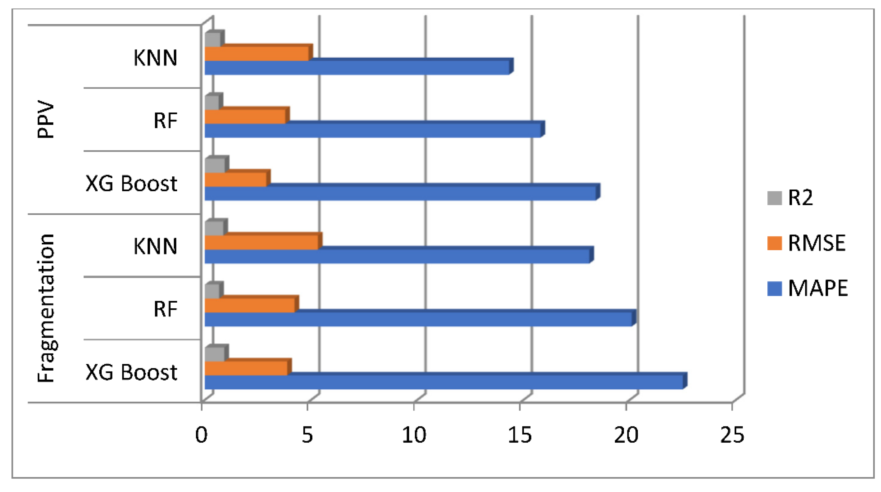
| MAPE | 24 | 22.5 | 21.2 | 20.1 | 19.2 | 18.1 |
| RMSE | 0.0854 | 3.873 | 0.0021 | 4.221 | 0.0031 | 5.321 |
| R2 | 0.953 | 0.9125 | 0.89 | 0.67 | 0.9 | 0.87 |
| Peak Particle Velocity | ||||||
| MAPE | 19 | 18.4 | 17.5 | 15.8 | 16.9 | 14.32 |
| RMSE | 0.0056 | 2.8890 | 0.0041 | 3.78 | 0.0886 | 4.88 |
| R2 | 0.96 | 0.932 | 0.79 | 0.65 | 0.83 | 0.72 |
Publisher’s Note: MDPI stays neutral with regard to jurisdictional claims in published maps and institutional affiliations. |
© 2022 by the authors. Licensee MDPI, Basel, Switzerland. This article is an open access article distributed under the terms and conditions of the Creative Commons Attribution (CC BY) license (https://creativecommons.org/licenses/by/4.0/).
Share and Cite
Chandrahas, N.S.; Choudhary, B.S.; Teja, M.V.; Venkataramayya, M.S.; Prasad, N.S.R.K. XG Boost Algorithm to Simultaneous Prediction of Rock Fragmentation and Induced Ground Vibration Using Unique Blast Data. Appl. Sci. 2022, 12, 5269. https://0-doi-org.brum.beds.ac.uk/10.3390/app12105269
Chandrahas NS, Choudhary BS, Teja MV, Venkataramayya MS, Prasad NSRK. XG Boost Algorithm to Simultaneous Prediction of Rock Fragmentation and Induced Ground Vibration Using Unique Blast Data. Applied Sciences. 2022; 12(10):5269. https://0-doi-org.brum.beds.ac.uk/10.3390/app12105269
Chicago/Turabian StyleChandrahas, N. Sri, Bhanwar Singh Choudhary, M. Vishnu Teja, M. S. Venkataramayya, and N. S. R. Krishna Prasad. 2022. "XG Boost Algorithm to Simultaneous Prediction of Rock Fragmentation and Induced Ground Vibration Using Unique Blast Data" Applied Sciences 12, no. 10: 5269. https://0-doi-org.brum.beds.ac.uk/10.3390/app12105269