
Estimation of Thickness and Speed of Sound for Transverse Cortical Bone Imaging Using Phase Aberration Correction Methods: An In Silico and Ex Vivo Validation Study


Abstract
:1. Introduction
2. Materials and Methods
2.1. Numerical Ultrasound Propagation Model
2.1.1. Reference Bone Model: Flat Bone Plate
2.1.2. Bone Curvature
2.1.3. Bone Tilt
2.1.4. Material Inhomogeneity: Cortical Pores
2.2. Ex Vivo Measurement on a Human Tibia Bone
2.3. Signal Processing
2.3.1. Reference Bone Model: Flat Bone Plate
2.3.2. Phase Aberration Correction
2.4. Statistics
3. Results
3.1. Numerical Simulations
3.1.1. Effect of Bone Curvature
3.1.2. Effect of Bone Tilt
3.1.3. Effect of Material Inhomogeneities
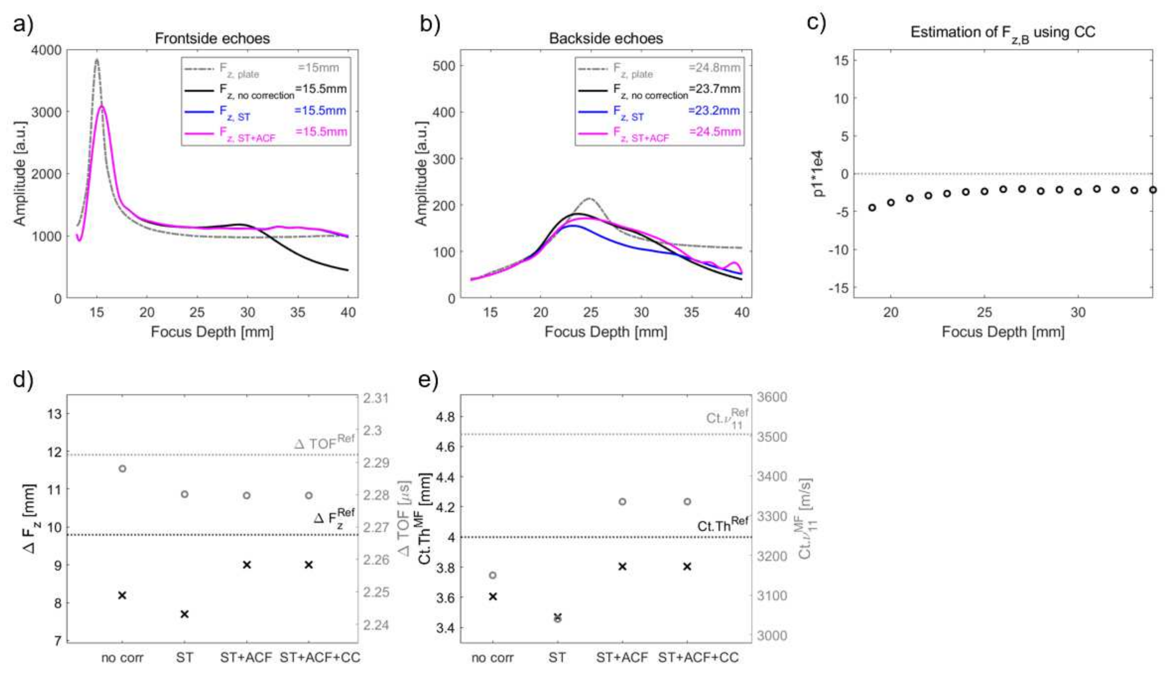
3.1.4. Overall Effect of PAC
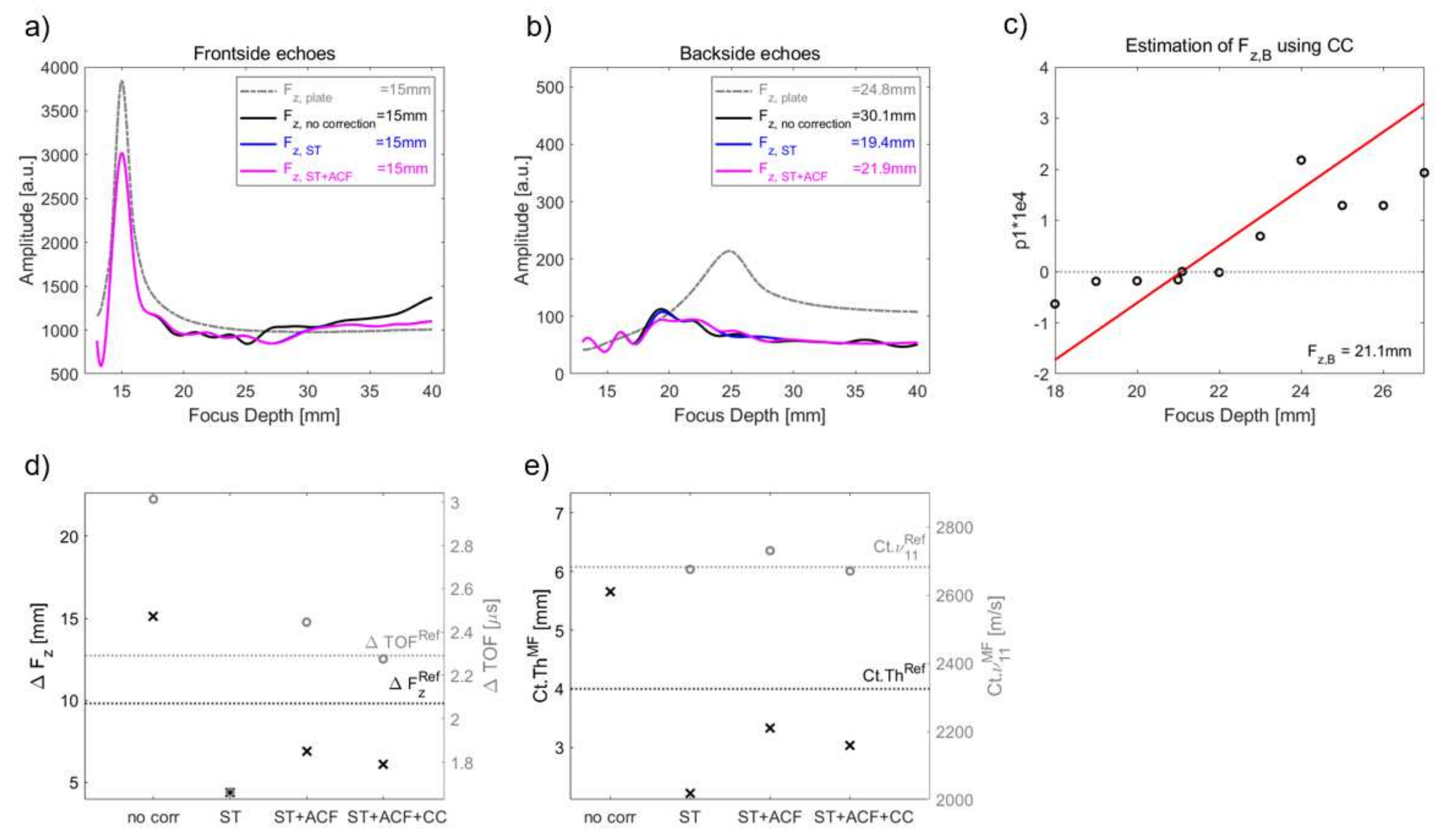
3.2. Ex-Vivo Multi-Focus Measurement
4. Discussion
4.1. Numerical Simulation
4.1.1. Effect of Bone Curvature
4.1.2. Effect of Bone Tilt
4.1.3. Effect of Material Inhomogeneities
4.1.4. Combination of Phase Aberration Methods
4.2. Ex Vivo Measurement
4.3. Transition to In Vivo Application
4.4. Limitations
5. Conclusions
6. Patent
Author Contributions
Funding
Institutional Review Board Statement
Informed Consent Statement
Data Availability Statement
Acknowledgments
Conflicts of Interest
Appendix A. Effect of Aperture and Semi-Aperture Angle θ


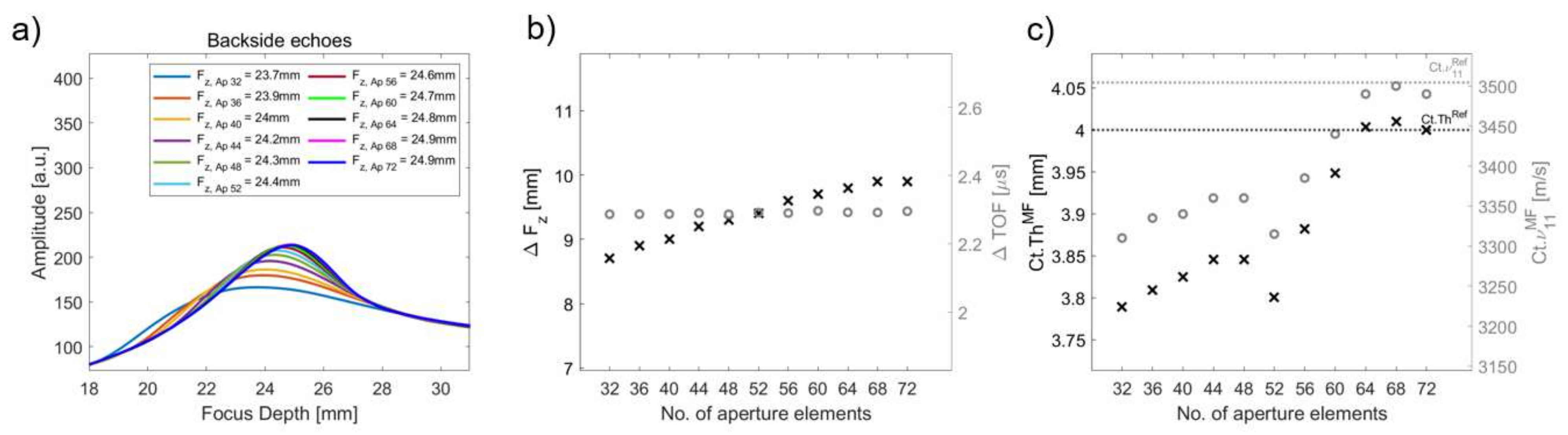
| Ap | ΔTOF [μs] | θ [°] | θcrit [°] | keffθ [°] | Ct.ThMF [mm] | RE [%] | Ct.ν11MF [m/s] | RE [%] |
|---|---|---|---|---|---|---|---|---|
| 32 | 2.287 | 11.75 | 26.95 | 11.75 | 3.79 | 5.27 | 3310 | 5.54 |
| 36 | 2.287 | 13.06 | 26.73 | 13.06 | 3.81 | 4.78 | 3335 | 4.83 |
| 40 | 2.287 | 13.77 | 26.69 | 13.77 | 3.82 | 4.39 | 3340 | 4.69 |
| 44 | 2.290 | 14.96 | 26.51 | 14.96 | 3.85 | 3.87 | 3360 | 4.12 |
| 48 | 2.286 | 16.19 | 26.51 | 26.51 | 3.85 | 3.87 | 3360 | 4.12 |
| 52 | 2.291 | 17.39 | 26.90 | 20.18 | 3.80 | 4.99 | 3315 | 5.40 |
| 56 | 2.290 | 18.50 | 26.30 | 17.61 | 3.88 | 2.96 | 3385 | 3.40 |
| 60 | 2.297 | 19.65 | 25.85 | 14.97 | 3.95 | 1.30 | 3440 | 1.83 |
| 64 | 2.292 | 20.77 | 25.38 | 12.46 | 4.00 | 0.01 | 3490 | 0.41 |
| 68 | 2.292 | 21.87 | 24.92 | 13.12 | 4.01 | 0.25 | 3500 | 0.21 |
| 72 | 2.296 | 23.03 | 25.45 | 13.82 | 4.00 | 0.01 | 3490 | 0.41 |
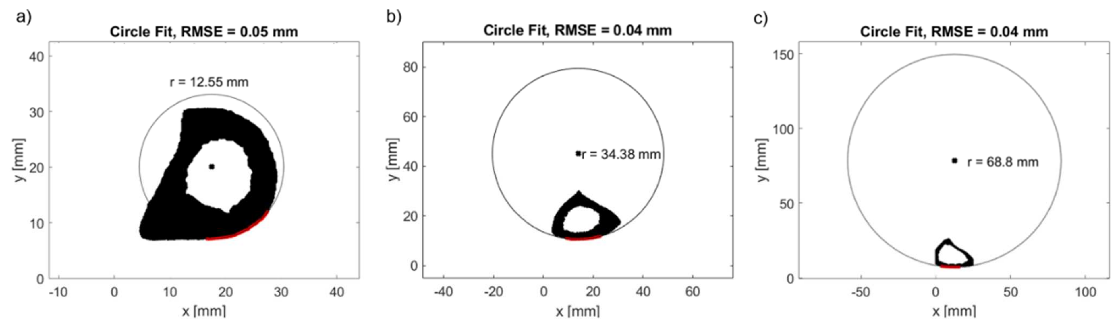
Appendix B. Estimation of Bone Curvature on HR-pQCT Bone Images

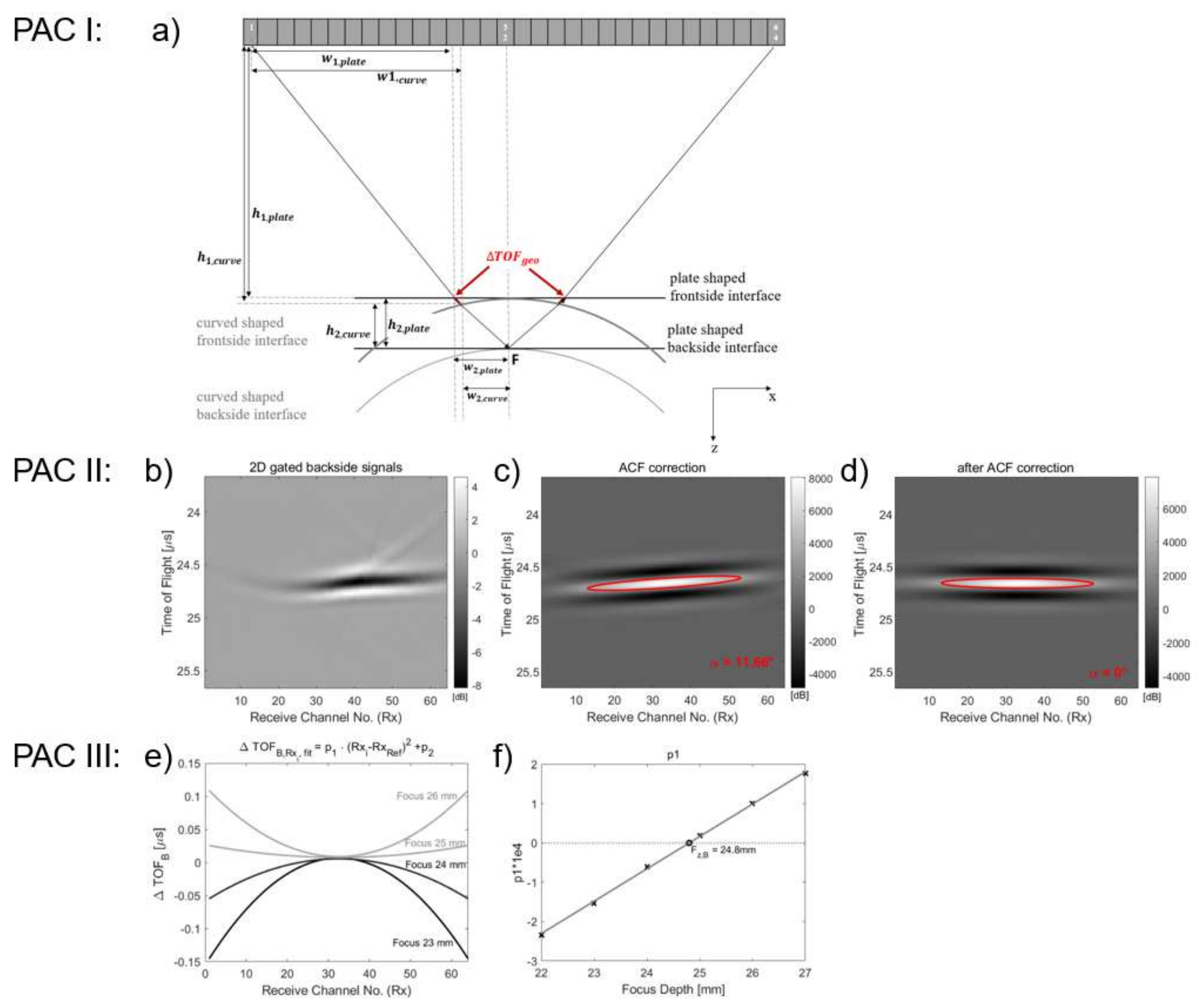
Appendix C. Phase Aberration Correction (PAC) Methods
Appendix C.1. PAC I: Time-Shift Correction Based on Periosteal Bone Surface Geometry, Surface Time Correction (ST)
Appendix C.2. PAC II: Tilt Correction (ACF)
Appendix C.3. PAC III: Cross-Correlation (CC)

Appendix D. Results
| Effect of. | Model Abbreviation | Curvature Radius r (mm) | Lateral Shift to Beam Axis dx (mm) | Bone Surface Tilt (°) | Porosity [%] |
|---|---|---|---|---|---|
| flat plate | 10,000 | 0 | 0 | 0 | |
| curvature | r60dx0 | 60 | 0 | 0 | 0 |
| r50dx0 | 50 | 0 | 0 | 0 | |
| r40dx0 | 40 | 0 | 0 | 0 | |
| r30dx0 | 30 | 0 | 0 | 0 | |
| r20dx0 | 20 | 0 | 0 | 0 | |
| curvature | r40dx1.11 | 40 | 1.11 | 1.4 | 0 |
| and | r40dx2.11 | 40 | 2.11 | 3.1 | 0 |
| tilt | r40dx3.11 | 40 | 3.11 | 4.5 | 0 |
| r40dx4.11 | 40 | 4.11 | 5.9 | 0 | |
| r40dx5.11 | 40 | 5.11 | 7.4 | 0 | |
| r40dx6.11 | 40 | 6.11 | 8.9 | 0 | |
| curvature | r40dx0Po2 | 40 | 0 | 0 | 2 |
| and | r40dx0Po4 | 40 | 0 | 0 | 4 |
| porosity | r40dx0Po6 | 40 | 0 | 0 | 6 |
| r40dx0Po8 | 40 | 0 | 0 | 8 | |
| r40dx0Po10 | 40 | 0 | 0 | 10 | |
| r40dx0Po12 | 40 | 0 | 0 | 12 | |
| r40dx0Po14 | 40 | 0 | 0 | 14 | |
| r40dx0Po16 | 40 | 0 | 0 | 16 | |
| r40dx0Po18 | 40 | 0 | 0 | 18 | |
| r40dx0Po20 | 40 | 0 | 0 | 20 |
| Model | Ct.ν11Ref [m/s] |
|---|---|
| r40dx0Po2 | 3428.6 |
| r40dx0Po4 | 3321.8 |
| r40dx0Po6 | 3189.4 |
| r40dx0Po8 | 3127.0 |
| r40dx0Po10 | 3038.0 |
| r40dx0Po12 | 2953.8 |
| r40dx0Po14 | 2848.7 |
| r40dx0Po16 | 2774.6 |
| r40dx0Po18 | 2704.2 |
| r40dx0Po20 | 2681.6 |
| Model | Correction | Ct.ThMF [mm] | RECt.Th [%] | Ct.ν11MF [m/s] | RECt.ν11 [%] |
|---|---|---|---|---|---|
| flat plate | No | 4.00 | 0.01 | 3490 | 0.41 |
| (reference) | ST | 4.00 | 0.01 | 3490 | 0.41 |
| ST + ACF | 4.00 | 0.01 | 3490 | 0.41 | |
| ST + ACF + CC | 4.00 | 0.01 | 3490 | 0.41 | |
| r60dx0 | No | 3.77 | 5.77 | 3330 | 5.83 |
| ST | 3.99 | 0.32 | 3470 | 0.98 | |
| ST + ACF | 3.99 | 0.32 | 3470 | 0.98 | |
| ST + ACF + CC | 4.00 | 0.01 | 3490 | 0.41 | |
| r50dx0 | No | 3.72 | 6.91 | 3255 | 7.11 |
| ST | 3.98 | 0.48 | 3475 | 0.83 | |
| ST + ACF | 3.98 | 0.48 | 3475 | 0.83 | |
| ST + ACF + CC | 4.00 | 0.01 | 3495 | 0.26 | |
| r40dx0 | No | 3.65 | 8.70 | 3180 | 9.25 |
| ST | 3.96 | 1.07 | 3460 | 1.26 | |
| ST + ACF | 3.96 | 1.07 | 3460 | 1.26 | |
| ST + ACF + CC | 4.02 | 0.51 | 3510 | 0.16 | |
| r30dx0 | No | 3.57 | 10.80 | 3120 | 10.97 |
| ST | 3.94 | 1.49 | 3440 | 1.83 | |
| ST + ACF | 3.93 | 1.65 | 3445 | 1.69 | |
| ST + ACF + CC | 4.06 | 1.48 | 3545 | 1.16 | |
| r20dx0 | No | 3.37 | 15.66 | 2955 | 15.67 |
| ST | 3.82 | 4.49 | 3340 | 4.69 | |
| ST + ACF | 3.85 | 3.78 | 3360 | 4.12 | |
| ST + ACF + CC | 3.85 | 3.78 | 3360 | 4.12 | |
| r40dx1.11 | No | 3.67 | 8.26 | 3210 | 8.40 |
| ST | 3.96 | 0.91 | 3455 | 1.41 | |
| ST + ACF | 3.96 | 1.07 | 3460 | 1.26 | |
| ST + ACF + CC | 4.03 | 0.67 | 3505 | 0.02 | |
| r40dx2.11 | No | 3.69 | 7.66 | 3235 | 7.68 |
| ST | 3.93 | 1.65 | 3445 | 1.69 | |
| ST + ACF | 3.96 | 0.91 | 3455 | 1.41 | |
| ST + ACF + CC | 3.96 | 0.91 | 3455 | 1.41 | |
| r40dx3.11 | No | 3.67 | 7.50 | 3205 | 7.83 |
| ST | 3.79 | 5.23 | 3325 | 5.12 | |
| ST + ACF | 3.95 | 1.19 | 3465 | 1.12 | |
| ST + ACF + CC | 3.95 | 1.19 | 3465 | 1.12 | |
| r40dx4.11 | No | 3.64 | 8.99 | 3175 | 9.40 |
| ST | 3.58 | 10.45 | 3140 | 10.39 | |
| ST + ACF | 3.93 | 1.86 | 3445 | 1.69 | |
| ST + ACF + CC | 3.93 | 1.86 | 3445 | 1.69 | |
| r40dx5.11 | No | 3.61 | 9.84 | 3150 | 10.11 |
| ST | 3.47 | 13.28 | 3040 | 13.25 | |
| ST + ACF | 3.80 | 4.91 | 3335 | 4.83 | |
| ST + ACF + CC | 3.80 | 4.91 | 3335 | 4.83 | |
| r40dx6.11 | No | 3.47 | 13.37 | 3030 | 13.53 |
| ST | 3.29 | 17.74 | 2895 | 17.39 | |
| ST + ACF | 3.54 | 11.48 | 3110 | 11.25 | |
| ST + ACF + CC | 3.54 | 11.48 | 3110 | 11.25 | |
| r40dx0Po2 | No | 3.60 | 10.02 | 3065 | 10.60 |
| ST | 3.88 | 3.08 | 3310 | 3.46 | |
| ST + ACF | 3.90 | 2.45 | 3330 | 2.88 | |
| ST + ACF + CC | 3.93 | 1.83 | 3350 | 2.29 | |
| r40dx0Po4 | No | 4.39 | 9.67 | 3640 | 9.58 |
| ST | 3.82 | 4.57 | 3165 | 4.72 | |
| ST + ACF | 3.81 | 4.47 | 3170 | 4.57 | |
| ST + ACF + CC | 3.76 | 6.08 | 3135 | 5.62 | |
| r40dx0Po6 | No | 3.57 | 10.79 | 2830 | 11.27 |
| ST | 3.85 | 3.79 | 3050 | 4.37 | |
| ST + ACF | 3.85 | 3.87 | 3055 | 4.21 | |
| ST + ACF + CC | 3.92 | 1.92 | 3120 | 2.18 | |
| r40dx0Po8 | No | 3.54 | 11.49 | 2805 | 10.30 |
| ST | 3.79 | 5.27 | 3015 | 3.58 | |
| ST + ACF | 3.83 | 4.18 | 3010 | 3.74 | |
| ST + ACF + CC | 3.89 | 2.87 | 3055 | 2.30 | |
| r40dx0Po10 | No | 5.16 | 29.12 | 3950 | 30.02 |
| ST | 3.98 | 0.48 | 3030 | 0.26 | |
| ST + ACF | 3.95 | 1.24 | 3015 | 0.76 | |
| ST + ACF + CC | 3.98 | 0.48 | 3030 | 0.26 | |
| r40dx0Po12 | No | 5.58 | 39.69 | 4090 | 38.47 |
| ST | 3.86 | 3.46 | 2835 | 4.02 | |
| ST + ACF | 3.87 | 3.23 | 2830 | 4.19 | |
| ST + ACF + CC | 3.92 | 1.94 | 2870 | 2.84 | |
| r40dx0Po14 | No | 4.78 | 19.54 | 3440 | 20.76 |
| ST | 3.78 | 5.40 | 2760 | 3.11 | |
| ST + ACF | 3.78 | 5.40 | 2760 | 3.11 | |
| ST + ACF + CC | 3.78 | 5.40 | 2760 | 3.11 | |
| r40dx0Po16 | No | 4.82 | 20.55 | 3870 | 39.48 |
| ST | 3.79 | 5.36 | 2635 | 5.03 | |
| ST + ACF | 3.79 | 5.14 | 2630 | 5.21 | |
| ST + ACF + CC | 3.90 | 2.58 | 2695 | 2.87 | |
| r40dx0Po18 | No | 3.82 | 4.52 | 2585 | 4.41 |
| ST | 3.98 | 0.56 | 2680 | 0.89 | |
| ST + ACF | 3.97 | 0.79 | 2685 | 0.71 | |
| ST + ACF + CC | 3.83 | 4.21 | 2640 | 2.37 | |
| r40dx0Po20 | No | 5.65 | 41.24 | 3750 | 39.84 |
| ST | 2.22 | 44.45 | 2675 | 0.25 | |
| ST + ACF | 3.33 | 16.66 | 2730 | 1.80 | |
| ST + ACF + CC | 3.03 | 24.14 | 2670 | 0.43 |


References
- Miller, P.D.; Siris, E.S.; Barrett-Connor, E.; Faulkner, K.G.; Wehren, L.E.; Abbott, T.A.; Chen, Y.T.; Berger, M.L.; Santora, A.C.; Sherwood, L.M. Prediction of fracture risk in postmenopausal white women with peripheral bone densitometry: Evidence from the National Osteoporosis Risk Assessment. J. Bone Miner. Res. 2002, 17, 2222–2230. [Google Scholar] [CrossRef] [PubMed]
- Njeh, C.F.; Hans, D.; Li, J.; Fan, B.; Fuerst, T.; He, Y.Q.; Tsuda-Futami, E.; Lu, Y.; Wu, C.Y.; Genant, H.K. Comparison of six calcaneal quantitative ultrasound devices: Precision and hip fracture discrimination. Osteoporos. Int. 2000, 11, 1051–1062. [Google Scholar] [CrossRef] [PubMed]
- Lasaygues, P.; Ouedraogo, E.; Lefebvre, J.P.; Gindre, M.; Talmant, M.; Laugier, P. Progress towards in vitro quantitative imaging of human femur using compound quantitative ultrasonic tomography. Phys. Med. Biol. 2005, 50, 2633–2649. [Google Scholar] [CrossRef] [PubMed]
- Lasaygues, P. Assessing the cortical thickness of long bone shafts in children, using two-dimensional ultrasonic diffraction tomography. Ultrasound Med. Biol. 2006, 32, 1215–1227. [Google Scholar] [CrossRef] [PubMed] [Green Version]
- Bernard, S.; Monteiller, V.; Komatitsch, D.; Lasaygues, P. Ultrasonic computed tomography based on full-waveform inversion for bone quantitative imaging. Phys. Med. Biol. 2017, 62, 7011–7035. [Google Scholar] [CrossRef]
- Li, H.; Le, L.H.; Sacchi, M.D.; Lou, E.H. Ultrasound imaging of long bone fractures and healing with the split-step fourier imaging method. Ultrasound Med. Biol. 2013, 39, 1482–1490. [Google Scholar] [CrossRef]
- Zheng, R.; Le, L.H.; Sacchi, M.D.; Lou, E. Imaging Internal Structure of Long Bones Using Wave Scattering Theory. Ultrasound Med. Biol. 2015, 41, 2955–2965. [Google Scholar] [CrossRef]
- Schneider, J.; Ramiandrisoa, D.; Armbrecht, G.; Ritter, Z.; Felsenberg, D.; Raum, K.; Minonzio, J.G. In Vivo Measurements of Cortical Thickness and Porosity at the Proximal Third of the Tibia Using Guided Waves: Comparison with Site-Matched Peripheral Quantitative Computed Tomography and Distal High-Resolution Peripheral Quantitative Computed Tomography. Ultrasound Med. Biol. 2019, 45, 1234–1242. [Google Scholar] [CrossRef] [Green Version]
- Giangregorio, L.M.; Webber, C.E. Speed of sound in bone at the tibia: Is it related to lower limb bone mineral density in spinal-cord-injured individuals? Spinal Cord 2004, 42, 141–145. [Google Scholar] [CrossRef]
- Moilanen, P.; Maatta, M.; Kilappa, V.; Xu, L.; Nicholson, P.H.; Alen, M.; Timonen, J.; Jamsa, T.; Cheng, S. Discrimination of fractures by low-frequency axial transmission ultrasound in postmenopausal females. Osteoporos. Int. 2013, 24, 723–730. [Google Scholar] [CrossRef]
- Karjalainen, J.P.; Riekkinen, O.; Toyras, J.; Hakulinen, M.; Kroger, H.; Rikkonen, T.; Salovaara, K.; Jurvelin, J.S. Multi-site bone ultrasound measurements in elderly women with and without previous hip fractures. Osteoporos. Int. 2012, 23, 1287–1295. [Google Scholar] [CrossRef] [PubMed]
- Vallet, Q.; Bochud, N.; Chappard, C.; Laugier, P.; Minonzio, J.G. In Vivo Characterization of Cortical Bone Using Guided Waves Measured by Axial Transmission. IEEE Trans. Ultrason. Ferroelectr. Freq. Control 2016, 63, 1361–1371. [Google Scholar] [CrossRef] [PubMed] [Green Version]
- Casciaro, S.; Peccarisi, M.; Pisani, P.; Franchini, R.; Greco, A.; De Marco, T.; Grimaldi, A.; Quarta, L.; Quarta, E.; Muratore, M.; et al. An Advanced Quantitative Echosound Methodology for Femoral Neck Densitometry. Ultrasound Med. Biol. 2016, 42, 1337–1356. [Google Scholar] [CrossRef] [PubMed]
- Renaud, G.; Kruizinga, P.; Cassereau, D.; Laugier, P. In vivo ultrasound imaging of the bone cortex. Phys. Med. Biol. 2018, 63, 125010. [Google Scholar] [CrossRef] [PubMed]
- Armbrecht, G.; Nguyen Minh, H.; Massmann, J.; Raum, K. Pore-Size Distribution and Frequency-Dependent Attenuation in Human Cortical Tibia Bone Discriminate Fragility Fractures in Postmenopausal Women With Low Bone Mineral Density. JBMR Plus 2021, 5, e10536. [Google Scholar] [CrossRef]
- Goss, S.A.; Johnston, R.L.; Dunn, F. Comprehensive compilation of empirical ultrasonic properties of mammalian tissues. J. Acoust. Soc. Am. 1978, 64, 423–457. [Google Scholar] [CrossRef]
- Granke, M.; Grimal, Q.; Saied, A.; Nauleau, P.; Peyrin, F.; Laugier, P. Change in porosity is the major determinant of the variation of cortical bone elasticity at the millimeter scale in aged women. Bone 2011, 49, 1020–1026. [Google Scholar] [CrossRef]
- Di Paola, M.; Gatti, D.; Viapiana, O.; Cianferotti, L.; Cavalli, L.; Caffarelli, C.; Conversano, F.; Quarta, E.; Pisani, P.; Girasole, G.; et al. Radiofrequency echographic multispectrometry compared with dual X-ray absorptiometry for osteoporosis diagnosis on lumbar spine and femoral neck. Osteoporos. Int. 2019, 30, 391–402. [Google Scholar] [CrossRef]
- Nguyen Minh, H.; Du, J.; Raum, K. Estimation of Thickness and Speed of Sound in Cortical Bone Using Multifocus Pulse-Echo Ultrasound. IEEE Trans. Ultrason. Ferroelectr. Freq. Control 2020, 67, 568–579. [Google Scholar] [CrossRef]
- Iori, G.; Schneider, J.; Reisinger, A.; Heyer, F.; Peralta, L.; Wyers, C.; Gluer, C.C.; van den Bergh, J.P.; Pahr, D.; Raum, K. Cortical thinning and accumulation of large cortical pores in the tibia reflect local structural deterioration of the femoral neck. Bone 2020, 137, 115446. [Google Scholar] [CrossRef]
- Bjornerem, A.; Bui, Q.M.; Ghasem-Zadeh, A.; Hopper, J.L.; Zebaze, R.; Seeman, E. Fracture risk and height: An association partly accounted for by cortical porosity of relatively thinner cortices. J. Bone Miner. Res. 2013, 28, 2017–2026. [Google Scholar] [CrossRef] [PubMed]
- Greenfield, M.A.; Craven, J.D.; Wishko, D.S.; Huddleston, A.L.; Friedman, R.; Stern, R. The modulus of elasticity of human cortical bone: An in vivo measurement and its clinical implications. Radiology 1975, 115, 163–166. [Google Scholar] [CrossRef] [PubMed]
- Stegman, M.R.; Heaney, R.P.; Traversgustafson, D.; Leist, J. Cortical Ultrasound Velocity as an Indicator of Bone Status. Osteoporos. Int. 1995, 5, 349–353. [Google Scholar] [CrossRef] [PubMed]
- Yasuda, J.; Yoshikawa, H.; Tanaka, H. Phase aberration correction for focused ultrasound transmission by refraction compensation. Jpn. J. Appl. Phys. 2019, 58, SGGE22. [Google Scholar] [CrossRef]
- Bossy, E.; Talmant, M.; Laugier, P. Three-dimensional simulations of ultrasonic axial transmission velocity measurement on cortical bone models. J. Acoust. Soc. Am. 2004, 115, 2314–2324. [Google Scholar] [CrossRef]
- Sasso, M.; Haiat, G.; Yamato, Y.; Naili, S.; Matsukawa, M. Frequency dependence of ultrasonic attenuation in bovine cortical bone: An in vitro study. Ultrasound Med. Biol. 2007, 33, 1933–1942. [Google Scholar] [CrossRef]
- Rohrbach, D.; Lakshmanan, S.; Peyrin, F.; Langer, M.; Gerisch, A.; Grimal, Q.; Laugier, P.; Raum, K. Spatial distribution of tissue level properties in a human femoral cortical bone. J. Biomech. 2012, 45, 2264–2270. [Google Scholar] [CrossRef]
- Iori, G.; Schneider, J.; Reisinger, A.; Heyer, F.; Peralta, L.; Wyers, C.; Grasel, M.; Barkmann, R.; Gluer, C.C.; van den Bergh, J.P.; et al. Large cortical bone pores in the tibia are associated with proximal femur strength. PLoS ONE 2019, 14, e0215405. [Google Scholar] [CrossRef]
- Chappard, C.; Bensalah, S.; Olivier, C.; Gouttenoire, P.J.; Marchadier, A.; Benhamou, C.; Peyrin, F. 3D characterization of pores in the cortical bone of human femur in the elderly at different locations as determined by synchrotron micro-computed tomography images. Osteoporos. Int. 2013, 24, 1023–1033. [Google Scholar] [CrossRef]
- Bakalova, L.P.; Andreasen, C.M.; Thomsen, J.S.; Bruel, A.; Hauge, E.M.; Kiil, B.J.; Delaisse, J.M.; Andersen, T.L.; Kersh, M.E. Intracortical Bone Mechanics Are Related to Pore Morphology and Remodeling in Human Bone. J. Bone Miner. Res. 2018, 33, 2177–2185. [Google Scholar] [CrossRef] [Green Version]
- Haïat, G. Linear Ultrasonic Properties of Cortical Bone: In Vitro Studies. In Bone Quantitative Ultrasound; Laugier, P., Haïat, G., Eds.; Springer: Dordrecht, The Netherlands, 2011; pp. 331–360. [Google Scholar]
- Iori, G.; Heyer, F.; Kilappa, V.; Wyers, C.; Varga, P.; Schneider, J.; Grasel, M.; Wendlandt, R.; Barkmann, R.; van den Bergh, J.P.; et al. BMD-based assessment of local porosity in human femoral cortical bone. Bone 2018, 114, 50–61. [Google Scholar] [CrossRef] [PubMed]
- Burghardt, A.J.; Buie, H.R.; Laib, A.; Majumdar, S.; Boyd, S.K. Reproducibility of direct quantitative measures of cortical bone microarchitecture of the distal radius and tibia by HR-pQCT. Bone 2010, 47, 519–528. [Google Scholar] [CrossRef] [PubMed] [Green Version]
- Hudimac, A.A. Ray Theory Solution for the Sound Intensity in Water Due to a Point Source above It. J. Acoust. Soc. Am. 1957, 29, 916–917. [Google Scholar] [CrossRef]
- Bala, Y.; Zebaze, R.; Seeman, E. Role of cortical bone in bone fragility. Curr. Opin. Rheumatol. 2015, 27, 406–413. [Google Scholar] [CrossRef]
- Chevalley, T.; Bonjour, J.P.; van Rietbergen, B.; Ferrari, S.; Rizzoli, R. Fracture history of healthy premenopausal women is associated with a reduction of cortical microstructural components at the distal radius. Bone 2013, 55, 377–383. [Google Scholar] [CrossRef]
- Yang, L.; Udall, W.J.M.; McCloskey, E.V.; Eastell, R. Distribution of bone density and cortical thickness in the proximal femur and their association with hip fracture in postmenopausal women: A quantitative computed tomography study. Osteoporos. Int. 2014, 25, 251–263. [Google Scholar] [CrossRef]
- Mikolajewicz, N.; Bishop, N.; Burghardt, A.J.; Folkestad, L.; Hall, A.; Kozloff, K.M.; Lukey, P.T.; Molloy-Bland, M.; Morin, S.N.; Offiah, A.C.; et al. HR-pQCT Measures of Bone Microarchitecture Predict Fracture: Systematic Review and Meta-Analysis. J. Bone Miner. Res. 2020, 35, 446–459. [Google Scholar] [CrossRef]
- Wydra, A.; Malyarenko, E.; Shapoori, K.; Maev, R.G. Development of a practical ultrasonic approach for simultaneous measurement of the thickness and the sound speed in human skull bones: A laboratory phantom study. Phys. Med. Biol. 2013, 58, 1083–1102. [Google Scholar] [CrossRef]
- Njeh, C.F.; Saeed, I.; Grigorian, M.; Kendler, D.L.; Fan, B.; Shepherd, J.; McClung, M.; Drake, W.M.; Genant, H.K. Assessment of bone status using speed of sound at multiple anatomical sites. Ultrasound Med. Biol. 2001, 27, 1337–1345. [Google Scholar] [CrossRef]
- Talmant, M.; Kolta, S.; Roux, C.; Haguenauer, D.; Vedel, I.; Cassou, B.; Bossy, E.; Laugier, P. In vivo performance evaluation of bi-directional ultrasonic axial transmission for cortical bone assessment. Ultrasound Med. Biol. 2009, 35, 912–919. [Google Scholar] [CrossRef]
- Olszynski, W.P.; Brown, J.P.; Adachi, J.D.; Hanley, D.A.; Ioannidis, G.; Davison, K.S.; CaMos Research, G. Multisite quantitative ultrasound for the prediction of fractures over 5 years of follow-up: The Canadian Multicentre Osteoporosis Study. J. Bone Miner. Res. 2013, 28, 2027–2034. [Google Scholar] [CrossRef] [PubMed] [Green Version]
- Minonzio, J.G.; Bochud, N.; Vallet, Q.; Ramiandrisoa, D.; Etcheto, A.; Briot, K.; Kolta, S.; Roux, C.; Laugier, P. Ultrasound-Based Estimates of Cortical Bone Thickness and Porosity Are Associated With Nontraumatic Fractures in Postmenopausal Women: A Pilot Study. J. Bone Miner. Res. 2019, 34, 1585–1596. [Google Scholar] [CrossRef] [PubMed]
- Behrens, M.; Felser, S.; Mau-Moeller, A.; Weippert, M.; Pollex, J.; Skripitz, R.; Herlyn, P.K.; Fischer, D.C.; Bruhn, S.; Schober, H.C.; et al. The Bindex((R)) ultrasound device: Reliability of cortical bone thickness measures and their relationship to regional bone mineral density. Physiol. Meas. 2016, 37, 1528–1540. [Google Scholar] [CrossRef] [PubMed]
- Karjalainen, J.; Riekkinen, O.; Toyras, J.; Kroger, H.; Jurvelin, J. Ultrasonic assessment of cortical bone thickness in vitro and in vivo. IEEE Trans. Ultrason. Ferroelectr. Freq. Control 2008, 55, 2191–2197. [Google Scholar] [CrossRef] [PubMed]
- Iori, G.; Du, J.; Hackenbeck, J.; Kilappa, V.; Raum, K. Estimation of Cortical Bone Microstructure From Ultrasound Backscatter. IEEE Trans. Ultrason. Ferroelectr. Freq. Control 2021, 68, 1081–1095. [Google Scholar] [CrossRef] [PubMed]
- Anderson, M.E.; McKeag, M.S.; Trahey, G.E. The impact of sound speed errors on medical ultrasound imaging. J. Acoust. Soc. Am. 2000, 107, 3540–3548. [Google Scholar] [CrossRef]
- Hasegawa, H.; Nagaoka, R. Initial phantom study on estimation of speed of sound in medium using coherence among received echo signals. J. Med. Ultrason. 2019, 46, 297–307. [Google Scholar] [CrossRef]
- Lee, J.; Yoo, Y.; Yoon, C.; Song, T.K. A Computationally Efficient Mean Sound Speed Estimation Method Based on an Evaluation of Focusing Quality for Medical Ultrasound Imaging. Electronics 2019, 8, 1368. [Google Scholar] [CrossRef] [Green Version]
- Renaud, G.; Clouzet, P.; Cassereau, D.; Talmant, M. Measuring anisotropy of elastic wave velocity with ultrasound imaging and an autofocus method: Application to cortical bone. Phys. Med. Biol. 2020, 65, 235016. [Google Scholar] [CrossRef]
- Ursell, T. autocorr2d.m, MATLAB Central File Exchange. Available online: https://www.mathworks.com/matlabcentral/fileexchange/67348-autocorr2d (accessed on 3 December 2020).


| Abbreviation | Description |
|---|---|
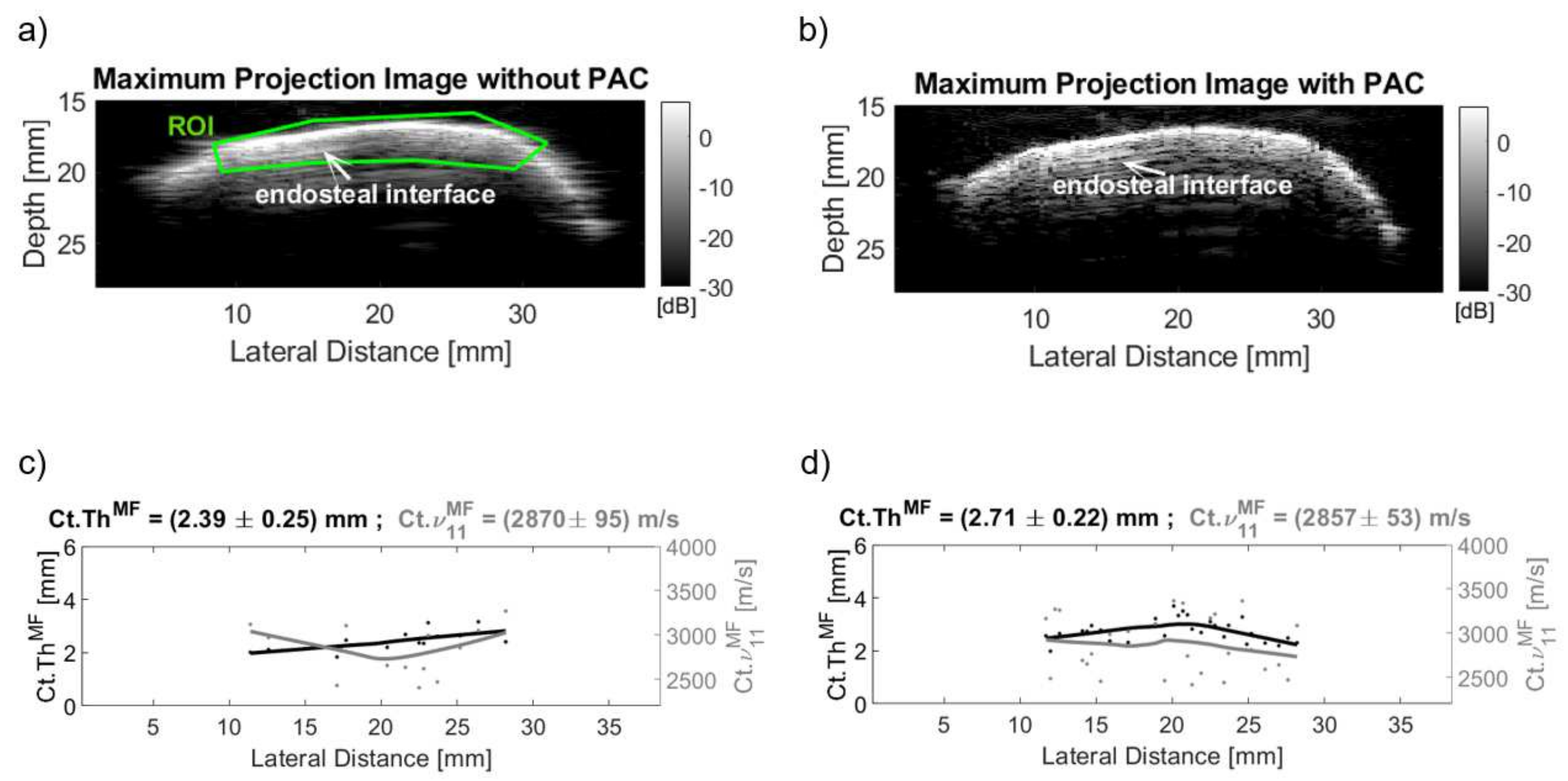
| Ct.Th | Cortical thickness |
| Ct.ν11 | Cortical compressional sound velocity propagating in the radial bone direction |
| νH2O | Speed of sound in water |
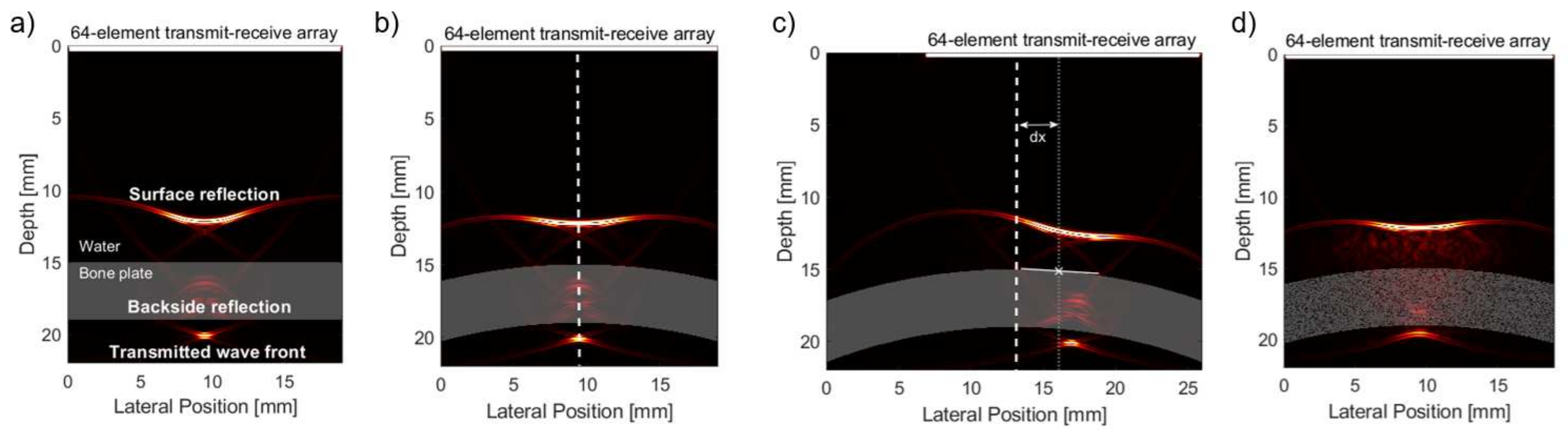
| dx | Lateral shift of center of mass of curved bone plate model relative to beam axis |
| r | Bone plate curvature radius |
| Ct.Po | Cortical porosity |
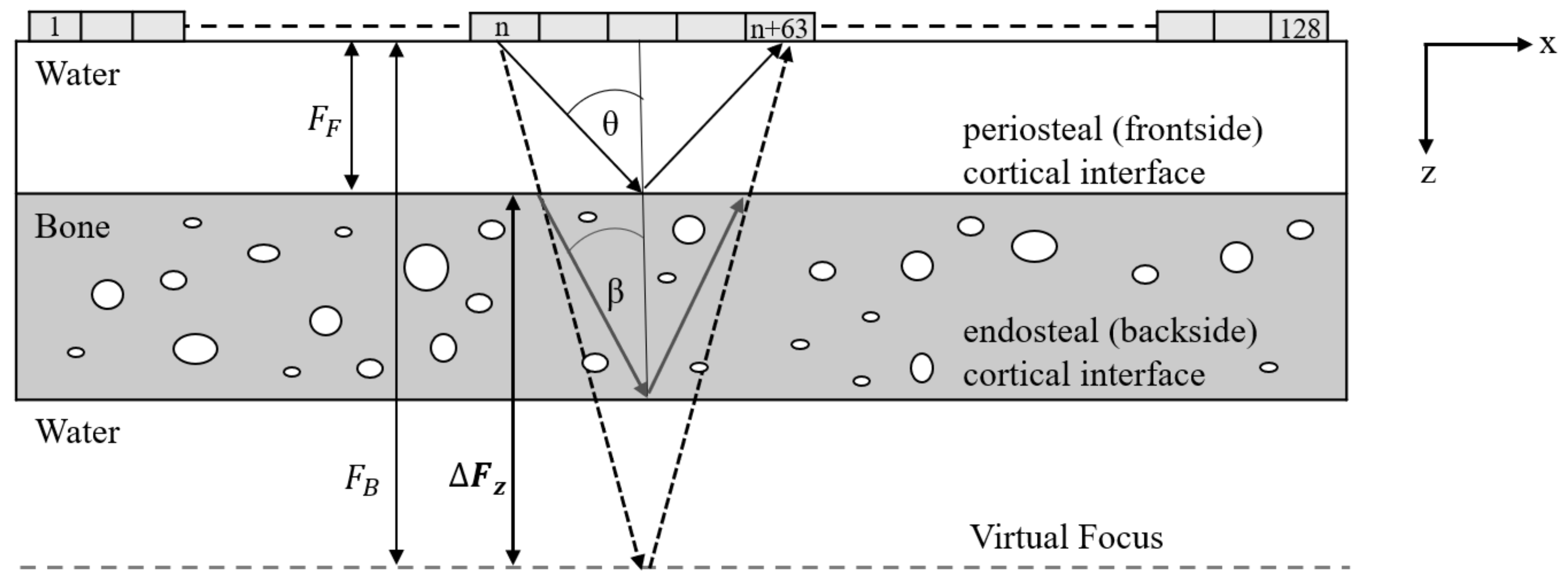
| Fz | Focus depth in z-direction |
| HF(Fz) | Amplitude of Hilbert-transformed envelope signal of beamformed frontside reflection at focus depth Fz |
| HB(Fz) | Amplitude of Hilbert-transformed envelope signal of beamformed backside reflection at focus depth Fz |
| FB | Front- and backside reflection |
| ΔTOF | Shift in time-of-flight between peak position of HF(Fz) and HB(Fz) |
| ΔFz | Shift in focus depth between peak position of HF(Fz) and HB(Fz) |
| Fz,B | Confocal focus depth position of backside reflection |
| θ | Semi-aperture angle of transmit and receive beams |
| keff | Correction factor keff for effective aperture keffθ |
| θcrit | Critical angle based on Snell’s law |
| Δθ | Difference of the semi-aperture angle to the critical angle |
| Txi, Rxi | Transmit or receive channel number |
| Rxref | Reference receive channel with maximum amplitude at envelope signal of pre-beamformed backside reflection |
| Vgb | Gated pre-beamformed backside reflection signals |
| VACF | Signal after using autocorrelation function (ACF) |
| |VACF| | Magnitude of the ACF signal |
| αACF | Inclination angle of the fitted ellipsoid on VACF to the major semi-axis |
| ΔtACF | Time shift correction based on αACF |
| Bone | Pores/Water | |
|---|---|---|
| ρ [g/cm3] | 1.93 | 1.00 |
| c11 [GPa] | 23.7 | 2.25 |
| c22 [GPa] | 23.7 | 2.25 |
| c12 [GPa] | 9.5 | 2.25 |
| c66 [GPa] | 6.6 | 0 |
| ν11 [m/s] | 3504 | 1500 |
| α [dB/mm] | 2.1 | 0.002 |
| Model | No PAC | ST | ST + ACF | ST + ACF + CC | |
|---|---|---|---|---|---|
| Ct.ThMF | Curved bone plate | 4.3% | 1.7% | 1.4% | 2.0% |
| Curved tilt bone plate | 2.3% | 7.3% | 4.3% (4.2%) * | 4.3% (1.1%) * | |
| Material inhomogeneity | 18.5% | 1.4% | 4.7% | 7.2% (1.9%) ** | |
| Ct.ν11MF | Curved bone plate | 4.3% | 1.6% | 1.4% | 2.0% |
| Curved tilt bone plate | 2.3% | 7.1% | 4.2% (2.5%) * | 4.3% (0.8%) * | |
| Material inhomogeneity | 15.9% | 7.9% | 7.9% | 8.2% (7.9%) ** |
| Model | No PAC | ST | ST + ACF | ST + ACF + CC | |
|---|---|---|---|---|---|
| Ct.ThMF | Curved bone plate | 10.2% | 2.2% | 1.9% | 1.8% |
| Curved tilt bone plate | 9.6% | 10.3% | 5.2% (1.3%) * | 5.2% (1.2%) * | |
| Material inhomogeneity | 23.2% | 14.6% | 6.3% | 8.3% (3.5%) ** | |
| Ct.ν11MF | Curved bone plate | 10.4% | 2.4% | 2.1% | 1.9% |
| Curved tilt bone plate | 9.8% | 10.1% | 5.1% (1.4%) * | 5.1% (1.2%) * | |
| Material inhomogeneity | 25.3% | 3.4% | 3.4% | 2.8% (3.0%) ** |
| Correction | Precision | Accuracy | |
|---|---|---|---|
| Ct.ThMF | No | 17.4% | 17.1% |
| ST | 10.3% | 11.2% | |
| ST + ACF | 4.1% | 5.2% | |
| ST + ACF + CC | 5.7% (2.1%) * | 6.3% (2.6%) * | |
| Ct.ν11MF | No | 11.6% | 18.5% |
| ST | 9.5% | 5.9% | |
| ST + ACF | 9.5% | 3.7% | |
| ST + ACF + CC | 9.8% (9.6%) * | 3.4% (2.3%) * |
Publisher’s Note: MDPI stays neutral with regard to jurisdictional claims in published maps and institutional affiliations. |
© 2022 by the authors. Licensee MDPI, Basel, Switzerland. This article is an open access article distributed under the terms and conditions of the Creative Commons Attribution (CC BY) license (https://creativecommons.org/licenses/by/4.0/).
Share and Cite
Nguyen Minh, H.; Muller, M.; Raum, K. Estimation of Thickness and Speed of Sound for Transverse Cortical Bone Imaging Using Phase Aberration Correction Methods: An In Silico and Ex Vivo Validation Study. Appl. Sci. 2022, 12, 5283. https://0-doi-org.brum.beds.ac.uk/10.3390/app12105283
Nguyen Minh H, Muller M, Raum K. Estimation of Thickness and Speed of Sound for Transverse Cortical Bone Imaging Using Phase Aberration Correction Methods: An In Silico and Ex Vivo Validation Study. Applied Sciences. 2022; 12(10):5283. https://0-doi-org.brum.beds.ac.uk/10.3390/app12105283
Chicago/Turabian StyleNguyen Minh, Huong, Marie Muller, and Kay Raum. 2022. "Estimation of Thickness and Speed of Sound for Transverse Cortical Bone Imaging Using Phase Aberration Correction Methods: An In Silico and Ex Vivo Validation Study" Applied Sciences 12, no. 10: 5283. https://0-doi-org.brum.beds.ac.uk/10.3390/app12105283