Applications of Operational Modal Analysis in Gearbox and Induction Motor, Based on Random Decrement Technique and Enhanced Ibrahim Time Method

Abstract

There have been steadily growing requirements from the academia and industry, demanding non-invasive methods and reliable measurement systems of research devoted to operational mode analysis (OMA). Due to the simplicity of performing only structures surface vibration measurements, OMA is frequently applied in machine fault diagnosis (MFD) and structure health monitoring (SHM). OMA can handle big structures, such as bridges, buildings, machines, etc. However, there is still an open question: how to properly handle the harmonic effects of rotating components and the difficulty of closely estimating space modes are still a nightmare to deal with. Therefore, the main objective of this paper is to identify the structure of natural frequencies by the regeneration of frequency response functions (FRFs) for complex structures based on OMA. The novelty of our approach is to use the random decrement technique (RDT), correlation function estimation (CFE), and enhanced Ibrahim time method (EITM) to overcome OMA’s difficulties and limitations. To reduce further rotational harmonics effects, gear mesh and side band frequencies, digital signal processing techniques based on notching filters, and liftering analysis techniques were also used. All the experiments were performed at the laboratory test rig and conducted by using three accelerometers, one impedance hammer, one force sensor, and one data acquisition board. To reduce data’s variabilities, each test was measured three times for 5 min. The data sampling frequency for all the experiments was 25.6 kHz. To validate the proposed methodology, extensive OMA tests were performed for the generation of FRFs. The measured objects were a steel bar, induction motor, and gearbox. Five structural natural frequencies for the induction motor and eight structural natural frequencies for the gearbox were generated, respectively.

1. Introduction

OMA is also known as ambient modal identification, ambient modal analysis, and output modal analysis. No matter the name, the main idea is the same: it aims to identify the structure’s dynamical parameters, based only on the vibration measurements, when the machines are under its operating conditions.

Scopus, Elsevier, IEEE, and SpringerLink were selected for the bibliography studies. Due to a widespread literature, research related to the OMA’s development was restricted to the last 19 years. Initially, let us introduce that OMA’s techniques can be classified by mainly two properties [1]: (1) time-domain and -domain, (2) non-bayesian (stochastic subspace identification), and bayesian (correlation function and spectral density). In our case, the literature review will be focused, especially, on the selected methods RDT, CFE, and EITD.

In this regard, one important tasks was carried out by P. Mohanty et al. in 2004 [2]; they studied the OMA in the presence of harmonic excitation. One difficulty was that, if the structure’s natural frequency is closed with the harmonic excitation, it fails to accurately identify the modal parameters. To properly identify the natural frequencies, they proposed a modification of the least-square complex exponential (LSCE), to identify the procedure to include explicitly harmonic signals. The measurement object was a beam with random excitation and several multi-harmonics loads. The applied system was a SIMO system, and they used an enhanced variant of Ibrahim time method (ITM) and LSCE. By applying OMA, it was still a major challenge to handle the MIMO systems and close spaced modes. The reduction of harmonics was studied by P. Mohanty et al. in 2004 [3]; they further studied the inclusion of harmonic excitation in OMA, using a new approach of EITM. In this case, they know a priori the harmonic excitation, and it was able to successfully detect the natural frequencies and damping data. The study’s object was a steel plate. J. Rodrigues et al. in 2005 [4] studied the application on OMA based on RD, ITD, and frequency domain decomposition (FDD). The outcomes of their studies were the generation of natural frequencies of a civil structure. At present, however, there is a somewhat limited validation process to quantify the obtained results.

A new approach, introducing OMA’s technique, based on non-bayesian (stochastic subspace identification), was developed by Z. Lingmi et al. 2005 [5]; they performed an overview of OMA, with further analysis with four time approaches, i.e., ARMA model-based, NEXT, stochastic realization-based, and stochastic subspace approaches, as well as frequencies approaches, i.e., frequency domain decomposition (FDD).

The researchers developed a new approach, concerning blind source separation, for the detection of modal parameters for OMA applications. J. Antoni et al. in 2013 [6] studied the OMA and blind source separation, also known as the blind signal separation method, for the identification of modal parameters. The second-order blind source separation (SOBSS) was applied for the analysis procedure, and the applicability of the framework of SOBSS in OMA was established. It was also established that the theoretical connection of SOBSS and stochastic subspace identification (SSI) stays as one of the aims of reference in OMA.

The OMA’s research took a new turn with the application of maximum likelihood estimation (MLE), as data preprocessing by estimating modal parameters by F.J. Cara et al. in 2012 [7]. The experimental modal analysis is an iterative method to find maximum likelihood estimation (MLE), which can handle, in this case, the state space model’s parameters. However, the above method has two drawbacks: (a) slow convergence and (b) high dependence on the initial conditions. To solve the difficulties, a stochastic subspace and the initial conditions with random points were used. The research work performed by Si-Da Z et al. in 2014 [8] presented the maximum likelihood estimator (MLE) for its ability to identify the structural modal time–frequency domain parameters. The obtained results were based on two time–frequency functions: the bivariate orthogonal and bivariate power polynomials.

The eigensystem realization algorithm (ERA) is used to identify dynamical structure parameters, which is commonly used with natural excitation technique (NEXT) to identify modal parameters from ambient vibration. Zhang Y et al. in 2014 [9] applied the ERA, which is one of the most popular methods in civil engineering for dynamical structural identification parameters. These papers focused on spurious mode, mode energy estimating, and analysis of the stabilization diagram. A new criterion was proposed, the modal similarity index (MSI), to measure the reliability of the modes. The mode energy content was used to define the dominant mode.

The finite element method (FEM) was used by M.L. Aenlle et al. in 2013 [10], in order to determine the modal scaling in OMA, who introduced the modal scaling in OMA using the mass matrix of a finite element model (FEM). The developed algorithms were validated by numerical simulations on a planar bridge and cantilever beam.

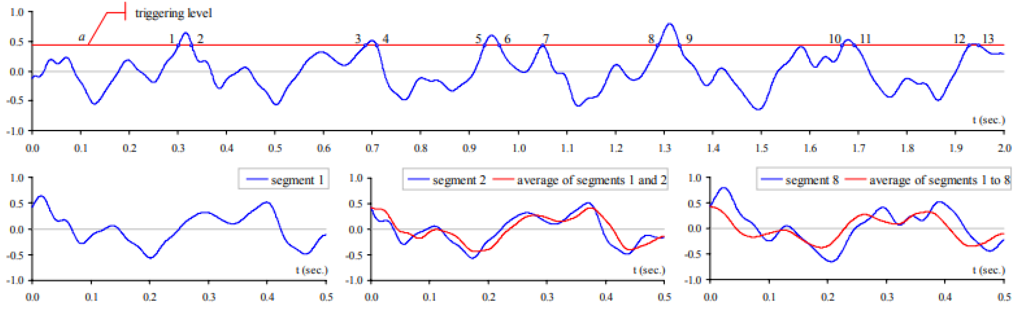
Y Zhang et al. [11] in 2015, applied a non-overlapped (RDT) for parameters identification with OMA. There was a drawback using RDT—due to averaging the raw data time segments, triggering the signal at the initial points of segmentation causes an overlap during triggering, which causes a residual excitation peak at the natural frequency. To solve the above difficulty, the following paper presented a non-overlapping technique to eliminate the peaks. R.B. Randall et al. in 2016 [12] studied a paper with the title, “Repressing the effects of variable speed harmonic orders in OMA”. This paper illustrated the machine shaft orders effects, which can disturb the OMA. To reduce difficulties, they studied three alternatives: (a) applied the time synchronous averaging (TSA), (b) the signals were transformed to order domain and applied a cepstral notch method to reduce speed harmonics and transformed it back to time-domain for OMA, (c) applied the raw vibration signal of an exponential short pass lifter to enhance the modal information. M. Salehi et al. in 2017 [13] performed a research study to extract modal parameters and compared them using various OMA methods, such as the frequency decomposition domain (FDD), enhanced frequency decomposition domain (EFDD), and stochastic subspace identification (SSI). A commercial software, PULSE^TM, was also used for validation proposes. The measured object was a four-stage centrifugal compressor. The identification of the of shaft harmonics were based on the values of the enhanced kurtosis analysis, However, the harmonics eliminations were not clear.

An extensive survey of cepstrum’s applications for structural dynamical identification parameters was presented by R.B. Randall et al. in 2019 [14]. The major idea of this method was to detect and remove periodic discrete frequency components. The main difficulty in OMA is to handle the periodic discrete frequency components, i.e., modulation side bands and harmonics. In some cases, the harmonics and side bands can be mistaken for slightly damped modes. In this case, a notch liftering technique was used, combined with an exponential lifter to remove/reduce the aforementioned difficulty.

There is an interesting and well-developed method for OMA’s applications, with locally preserving projections (LPP) and principal components analysis (PCA) methods, respectively. C. Wang et al. in 2019 [15] developed a new online operational method, based on vibration analysis, for the control of linear-time varying structures. The main idea was to overcome the limitations of resonance uncertainties of the OMA analysis by combining the idea of “forgetting factor weighting”, locally preserving projections (LPP), and eigenvector recursive PCA. The authors claimed that the methodology works faster, requires less memory space, and archives higher identification accuracy. In W. Fu et al.’s 2021 paper [16], further findings were developed. In [15], the method based on moving windows and locally preserving projection algorithms was proposed, in order to successfully identify the modal parameters with the OMA method.

F.B. Zahid et at. (2021) [17] carried out an extensive review of OMA techniques for in-service modal identification. The OMA studied techniques are: peak picking (PP), the basic assumption the modes are well-separated, and the damping is separated; frequency domain decomposition (FDD) can estimate the natural frequencies and closed space modes accurately; time-domain decomposition (TDD)—computationally efficient, but difficult to extract close spaced modal parameters; natural excitation technique (NEXT)—good ground to extend EMA into OMA, but difficulties in data processing; autoregressive moving average (ARMA)—output measurements can be used directly; the computationally intensive method; stochastic subspace identification (SSI)—high parameters estimation and accuracy; and the mathematically complex method. This paper performs an extensive literature review; however, there are methods that were not included in the analysis, such as the RDT and ITD methods, respectively.

We can draw some remarks, related to the literature review. OMA techniques showed a lot of potential, due to the simplicity in performing vibration measurements. It can perform under running conditions. There are no necessary extra requirements for measurement conditions, such as EMA. It can handle big structures, such as bridges, buildings, machines, etc. However, there are still open questions. What kind of algorithm can be used? How is it related the structure complexity of the algorithm election choice? Is there any framework for applying a certain algorithm to a certain type of structure? There is still a lot of research to cover the state-of-the-art of OMA. Therefore, this research paper aims to put two of most popular methods, RDT [1,4,11,18] and EITM [3], into perspective, applying them in steel plate in the early stage of development. The validation process was carried out in a steel beam, induction motor, and gearbox. The windowing technique was also applied, similar to that which was used in paper [15]. However, in this case, a liftering technique was used to eliminate the harmonic effects. Different frequency bands were also used as a pre-processing technique to reduce noise.

Due to the simplicity of performing only surface structure vibration measurements, OMA is frequently applied in machine diagnosis and health condition monitoring [1,2,7,19,20]. However, there is still a lot of research to cover OMA’s major drawbacks, i.e., the reduction of harmonic’s effects, accurate handling of MIMO systems, and difficulty in estimating close space modes. Therefore, our research approach intends to overcome OMA’s difficulties with three of most popular methods: RDT, CFE, and EITM. The measured raw data was pre-processed by the RD technique to obtain free decay responses before they were introduced to EITD.

The rest of this paper is structured as follows: Section 2 presents the methods and procedure analysis (EMA, RDT, CFE, EITM, and measurement set up). Section 3 contains the results and analysis. Section 4 presents the discussions. Finally, the Section 5 is presented.

2. Methods and Procedure Analysis

In this section, EMA, RDM, CFE, and EITM are presented. This section also includes the measurement setup and procedure analysis.

2.1. Experimental Modal Analysis (EMA)

The EMA is an effective tool for machine diagnosis and structure health monitoring. EMA determines the dynamical parameters of the structure by obtaining the frequency transform function, which contains the resonances, anti-resonances, and damping of the system. This method was used for the validation process, in order to compare the results of OMA. This method is well-established in the scientific area, so the readers are directly referring to [21].

2.2. Random Decrement Technique (RDT)

The RDT is a time-domain procedure, which was developed in the 1960s by NASA. It works when the structural responses are transformed into random decrement functions, which can be considered proportional to the free vibrations responses. The main objective of RDT is to identify the modal parameters of the structure from only the vibration response under machine running conditions, see Figure 1. This method works by finding a starting point (trigger) to start segmenting the measured signal. The higher the number of segments or samples of the signal to estimate the RD-signature, i.e., to get an average, the closer the RD-signature will be to the actual signal without noise [1].

2.3. Correlation Function Estimation (CFE)

The CFEs are a measure of the similarity between random signals. The CFE analyses the correlation function matrix by the well-known, direct method from the data response matrix [1]. The CFE matrices, at different time lags, are obtained in 3D. In our research work, the CFEs are used as interface functions to introduce the preprocessed data into EITM.

2.4. Enhance Ibrahim Time Method (EITM)

To identify the dynamic properties, the Ibrahim time-domain method (ITM) is one of the first techniques developed, while the systems/machines are under running conditions. There are several concerns with the OMA method, based on ITM, especially the difficulties regarding the detection of the resonances (closely to harmonics), due to rotating components. The standard ITD was initially developed for a simple input system, and only a simple decomposition analysis was permitted [1]. EITM was used to reduce the effects of closely spaced modes and apply for MIMO systems [1]. This limitation of the method can be evaded if we realize that the matrices can worked as Toeplitz block matrices, which essentially contain correlation data. This means that the MIMO version of the ITD can be obtained by EITD by calculating the Toeplitz arrays of all outputs [1].

The following equations describes the ITM’s analysis procedure [1].

$$y\left(t\right)=c_1{a}_1{e}^{{\lambda }_{1}k\Delta t}+c_2{a}_2{e}^{{\lambda }_{2}k\Delta t}=c_1{a}_1{\mu }_1{}^k+c_1{a}_1{\mu }_2{}^k$$

(1)

where $\Delta t$ is the time delay, λ_n are the continuous time resonances, $a$_n are the mode shapes, and ${\mu }_n$ are the discrete resonances. The following equation describes the Hankel matrix [1]:

$$\mathrm{H}=\left[\begin{array}{cccc}y\left(1\right)& y\left(2\right)& \dots & y\left(np-3\right)\\ y\left(2\right)& y\left(3\right)& \dots & y\left(np-2\right)\\ y\left(3\right)& y\left(4\right)& \dots & y\left(np-1\right)\\ y\left(4\right)& y\left(5\right)& \dots & y\left(np\right) \end{array}\right]=\left[\begin{array}{c}{\mathrm{H}}_1\\ {\mathrm{H}}_2\end{array}\right]$$

(2)

If the free decomposition has np numbers of data in the signal (taking into account H₁), it can be expressed as [1]:

$${\mathrm{H}}_1=\Psi \Lambda$$

(3)

where $\Psi$ is a matrix which contains the mode shapes.

$$\Psi =\left[\begin{array}{ccc}{a}_1& a_2& \dots \\ {\mu }_1{a}_1 & {\mu }_2{a}_2& \dots \end{array}\right]$$

(4)

$\Lambda$ is the matrix containing the discrete time poles raised to different powers and multiplied by the corresponding modal amplitudes [1].

$$\Lambda =\left[\begin{array}{cccc}{c}_1{\mu }_1^0& c_1{\mu }_1^1& \dots & c_1{\mu }_1^{np-3}\\ c_2{\mu }_2^0& c_2{\mu }_2^1& \dots & c_2{\mu }_2^{np-3}\\ ⋮& ⋮& & ⋮\end{array}\right]$$

(5)

The Hankel matrix H₂ can be expressed with a delay of two time steps:

$${\mathrm{H}}_2=\Psi {\left[{\mu }_n\right]}^2\Lambda$$

(6)

In order to eliminate expression $\Lambda$, Equations (1) and (3) can be used, and this gives:

$${\Psi }^{-1}{\mathrm{H}}_1={\mathrm{H}}_2{\Psi }^{-1}{\left[{\mu }_n\right]}^{-2}$$

(7)

Multiplying both sides of Equation (7) with $\Psi {\left[{\mu }_n\right]}^2$ gives:

$$\Psi {\left[{\mu }_n\right]}^2{\Psi }^{-1}{\mathrm{H}}_1={\mathrm{H}}_2$$

(8)

It is defined the system matrix:

$$\mathsf{A}=\Psi {\left[{\mu }_n\right]}^2{\Psi }^{-1}$$

(9)

Finally, the ITD estimation values can be seen in Equations (10)–(13) [1].

$${\mathsf{A}\mathrm{H}}_1={\mathrm{H}}_2$$

(10)

$$\widehat{{\mathrm{A}}_1}={\mathrm{H}}_2{\mathrm{H}}_1^T{({\mathrm{H}}_1{H}_1^T)}^{-1}$$

(11)

$$\widehat{{\mathrm{A}}_2}={\mathrm{H}}_2{\mathrm{H}}_2^T{({\mathrm{H}}_1{H}_2^T)}^{-1}$$

(12)

$$\widehat{A}=\left(\widehat{{\mathrm{A}}_1}+\widehat{{\mathrm{A}}_2}\right)/2$$

(13)

The standard ITD was initially developed for a simple input system, and only a simple decomposition analysis was permitted. This method’s limitation can be evaded if we realize that the matrices can worked as Toeplitz block matrices, which essentially contain correlation data. This means that the MIMO version of the ITD can be obtained by calculating the Toeplitz arrays of all output. For obtaining the EITD method, the readers may refer to more details in [1].

2.5. Measurement Set Up and Procedure Analysis

This section describes and illustrates the experimental set up and analysis procedure for all the experiments. The vibration data recording was carried out at our laboratory’s test rig for industrial innovation technology and robotics. One motor (WEG 2hp), one impact hammer (PCB 086c03), one force sensor, and three piezoelectric accelerometers (PCB 353B17) were also used to conduct the experiments. All the vibration signals were simultaneously digitized by using a NI-DAQ 9775. Experimental data were generated from a steel bar, gearbox, and induction motor. To have enough analysis data and reduce measurement variabilities, each test was measured three times for 5 min. The sampling frequency for all the experiments was about 25.6 kHz.

Figure 2 illustrates the gearbox used for the experiments, and it was a two-stage compound reverted gear train to be in-line. The spur gear E₁ had 17, E₂ had 40, E₃ had 13, and E₄ had 27 teeth, respectively.

Figure 3 denotes the measurement set up for EMA for an induction motor and gearbox. The tests were conducted using the impedance hammer, force sensor, and three accelerometers, which were mounted firmly on the steel bar, induction motor, and gearbox, respectively. It can be observed that the measured objects were suspended using soft springs, as shown in Figure 3. An impulse force hammer is a hammer equipped with a piezoelectric force sensor, and it is used in structural and modal analysis to stimulate a structure. Then, the EMA measured data will be used for validation proposes with OMA data.

The second set of measurements were carried out when the machines were running in normal conditions. Figure 4 illustrates OMA’s measurement set up for the induction motor, with mounted accelerometers. To measure the gearbox, the induction motor was connected to gearbox’s shaft for the generation of rotational speed. The gearbox’s measurement set up shows in Figure 5. The measurements were done with three speeds at 1800, 2400, and 3000 rpm, respectively. Signals were collected from the steel bar, induction motor, and gearbox.

Figure 6 illustrates the typical measured signals from the force impedance hammer and vibration response in the time-domain.

3. Analysis and Results

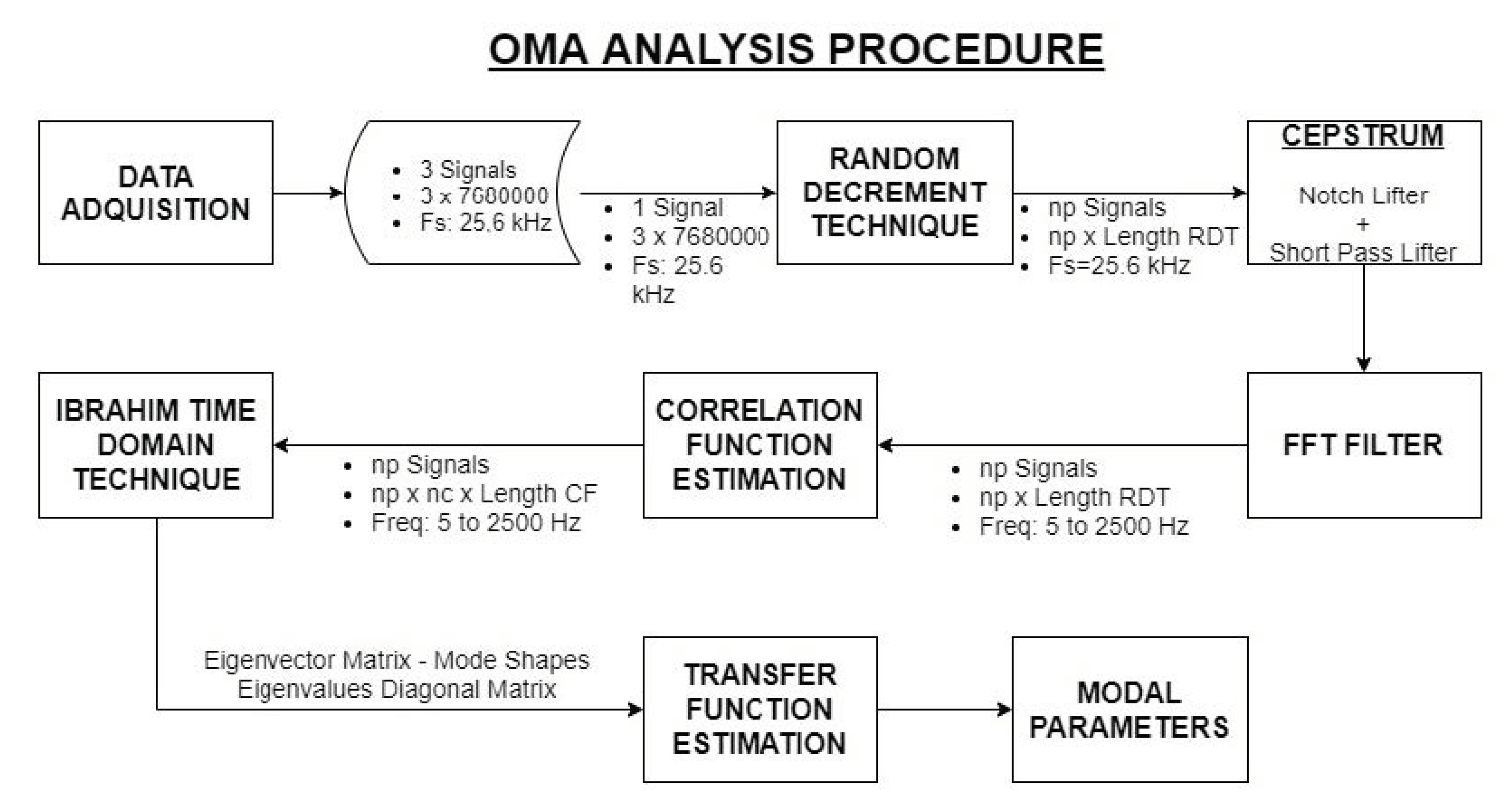
This section describes and illustrates the EMA and OMA methods, respectively. The overall schematic description, regarding the analysis procedure for regenerating the FRFs from the vibration responses, can be seen in Figure 7. The analysis part started with the pre-processing of the vibration data; an extensive reciprocating coherence analysis was carried out, in order to find out the best measurement points in the structure. The total measured length for each signal was around 768,000 samples. Thereafter, the RD technique procedure was applied to the raw signals, in order to obtain a matrix of 25 × 25,600.

To limit the range of interest, a digital low pass filter was used, and a notch filter was also applied to eliminate speed rotation harmonics. Furthermore, in order to eliminate the gear mesh contact frequencies, the cepstrum (filtering) technique was used. CFE, which has ability to extract interesting information about the modal characteristics of the signals, was also applied. Therefore, after the CFE, the obtained vectors were 25 × 25 × 16,385. Finally, the EITM analysis was performed to obtain the structural resonances, based on Brincker [1].

As it was observed in the development of this research work, to validate the proposed analysis process, we started from the design of an experiment with a simple structure to develop the final process with experiments using complex structures. The structure’s natural frequencies of the steel beam, induction motor, and gearbox were obtained through OMA.

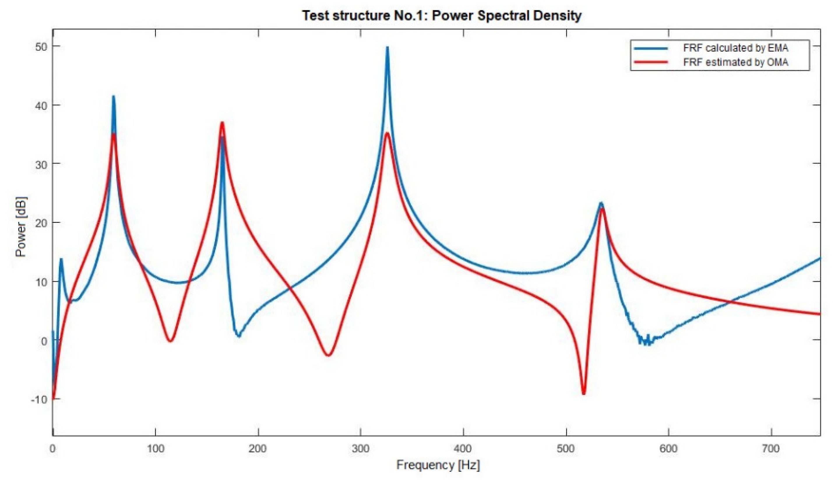
The measured and regenerated FRFs of the obtained results on the steel bar of the EMA and OMA measurements can be seen in Figure 8. It can be pointed out that the structure resonances are global parameters, which means the resonances do not change in frequency, due to input force placement. It can also be stressed out that the structure regenerate natural frequencies have almost the same frequencies as the measured ones; however, it seems that the anti-resonances have slightly variations or, in some cases, does not exist.

The steel bar’s regenerate structure natural frequencies for EMA and OMA are shown in

Table 1. Steel bar’s regenerate structure natural frequencies.

	Mode Number
	1	2	3	4	5
EMA [Hz]	8	59	165	326	534
OMA [Hz]	-	59	165	326	535

. The obtained results have high accuracy, except at 8 Hz. It was difficult to generate a FRF for that specific resonance frequency with precision.

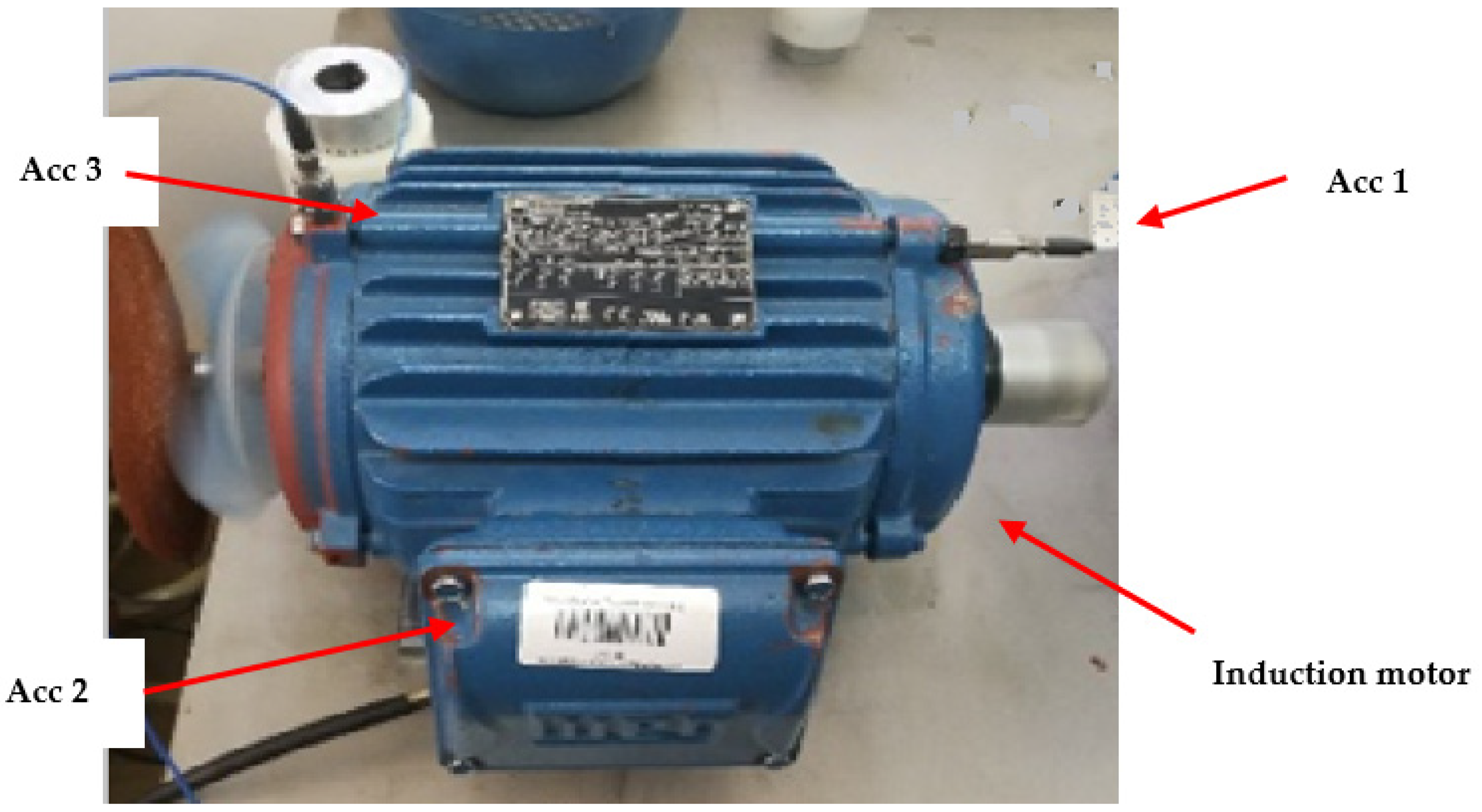
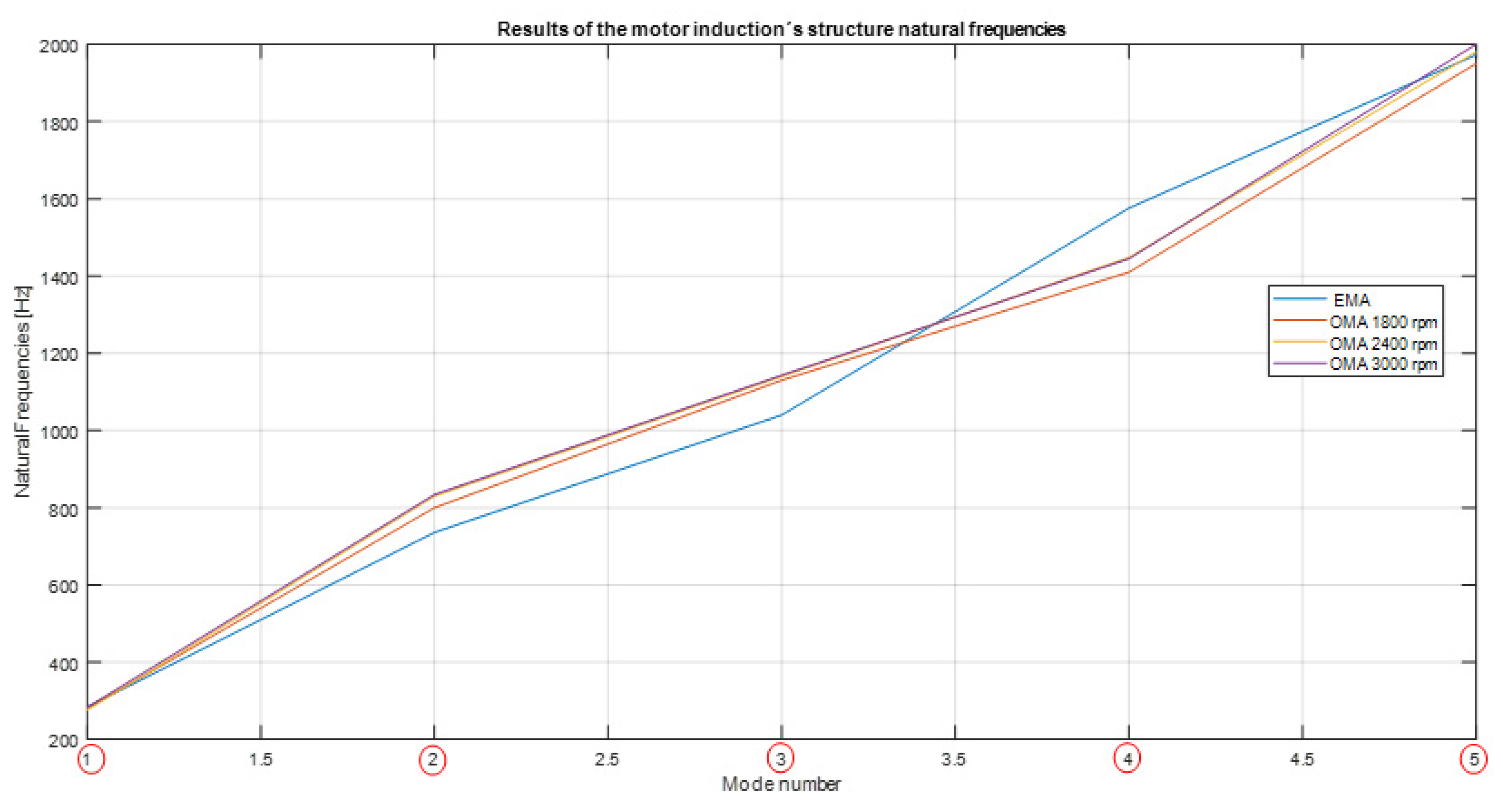
Figure 9 illustrates the obtained results of the regenerated natural frequencies of the induction motor at 1800, 2400, and 3000 rpm, respectively. The obtained results showed an overall consistency. However, it was quite difficult to regenerate the structure’s natural frequencies, between 600 to 900 Hz at 1800 rpm, with high precision.

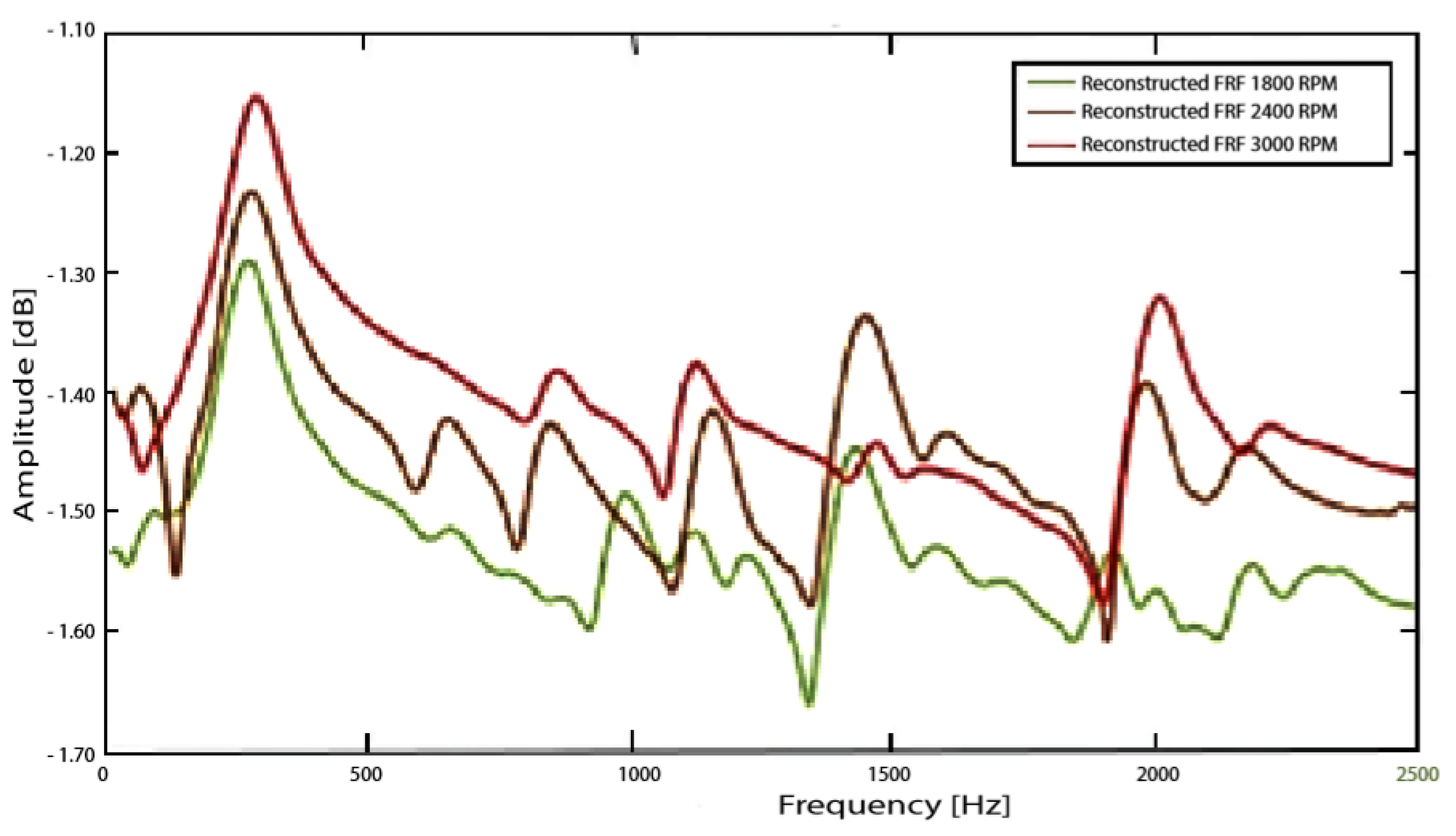
Five generated natural structure frequencies for the induction motor were detected. To quantify the precision of the obtained OMA’s results, Figure 10 denotes the comparison of the induction motor’s FRFs, with five modes at varying speeds (1800, 2400, and 3000 rpm). The highest accuracy was shown by mode one.

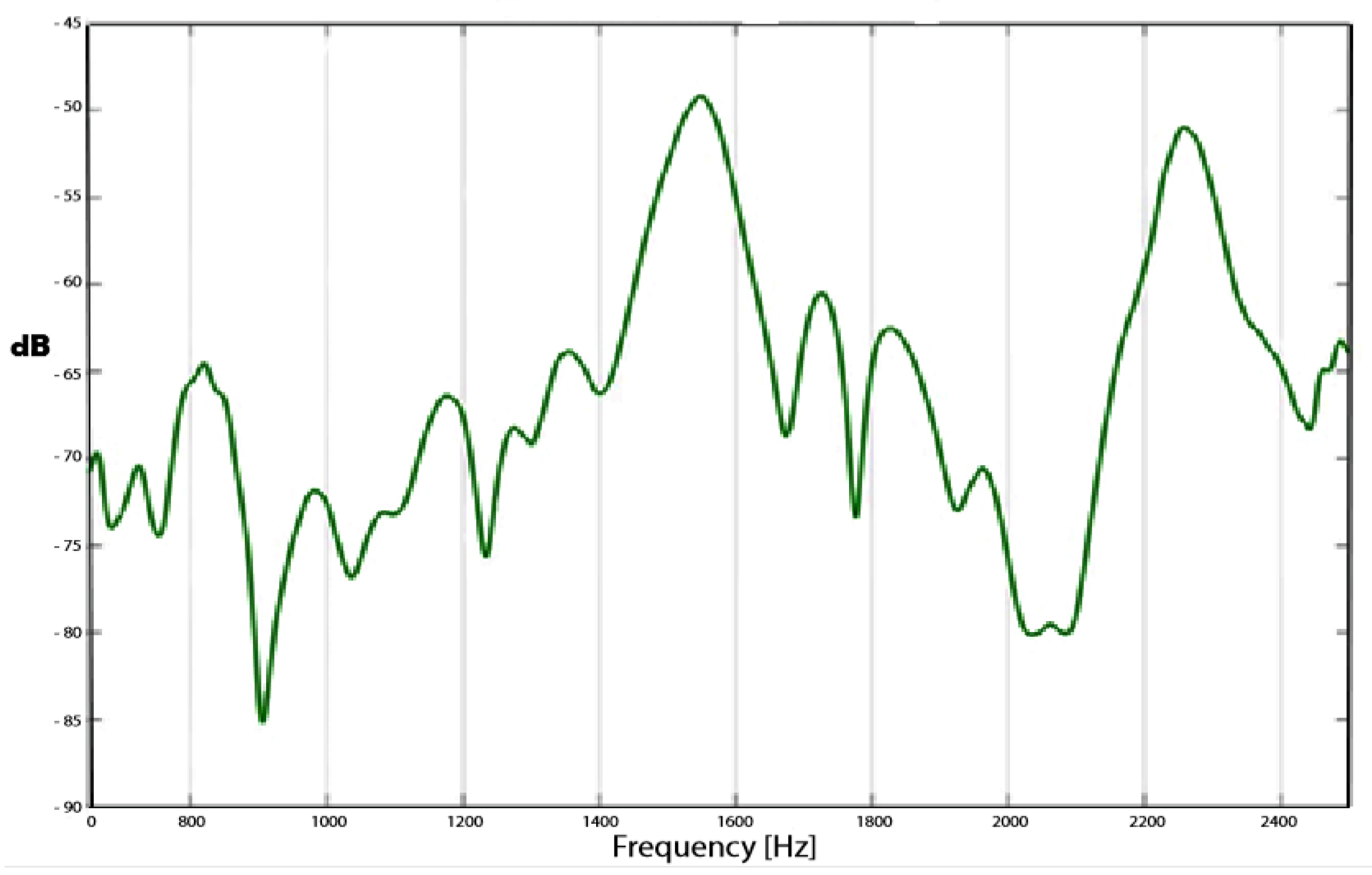
A typical gearbox’s regenerated transfer function at 3000 rpm can be seen in Figure 11.

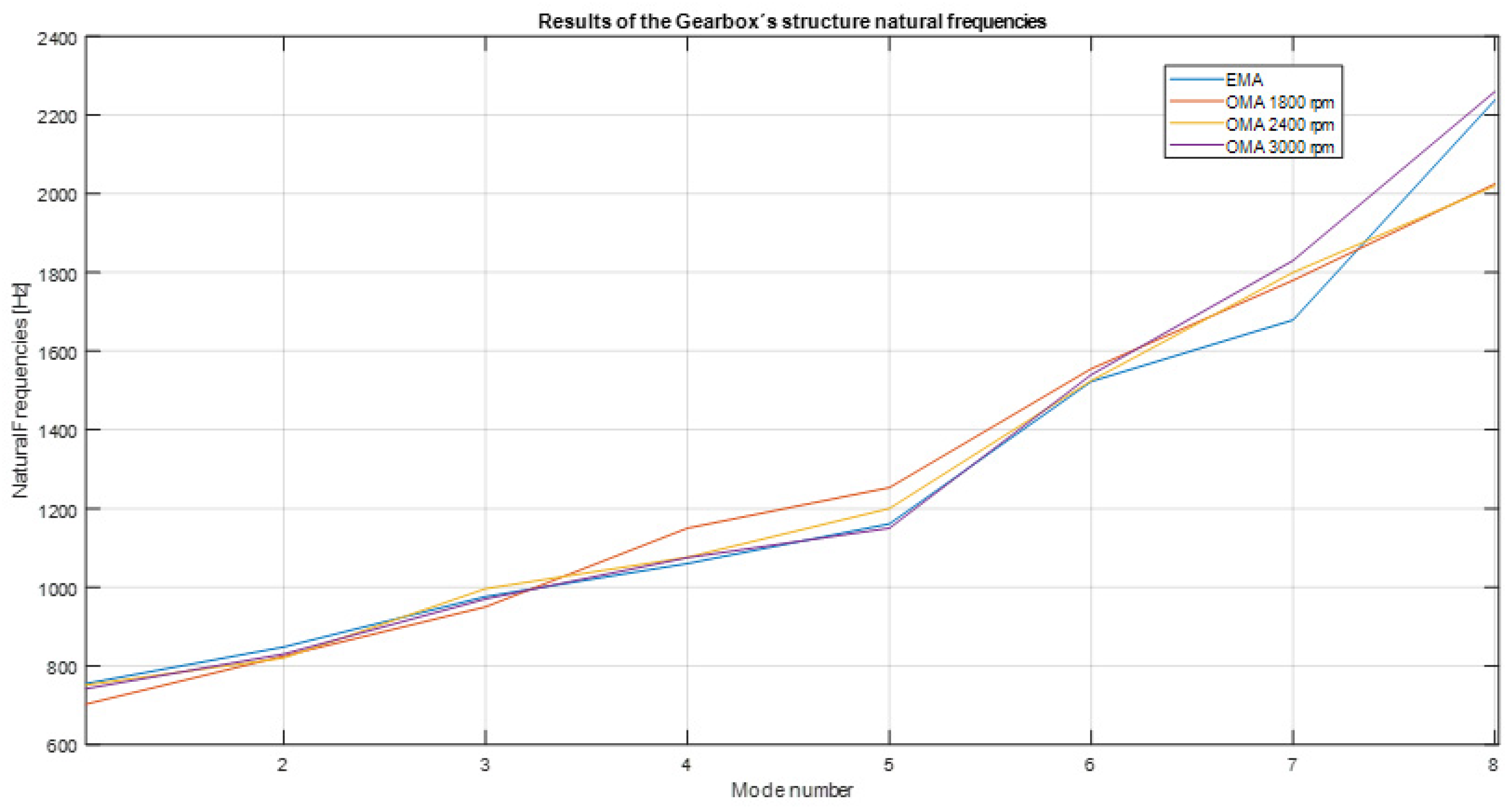
Figure 12 illustrates the obtained results of the gearbox structure’s natural frequencies with varying speeds. The first three regenerated modes have the highest precision; they can be used for machine diagnostics. In order to reduce the frequency dispersion for higher modes, we could determine a calibration curve to use to adjust the measurement values. An advanced equalization process and scaling of the generated FRFs [14], in order to increase the precision, could be the subject of future research.

4. Discussion

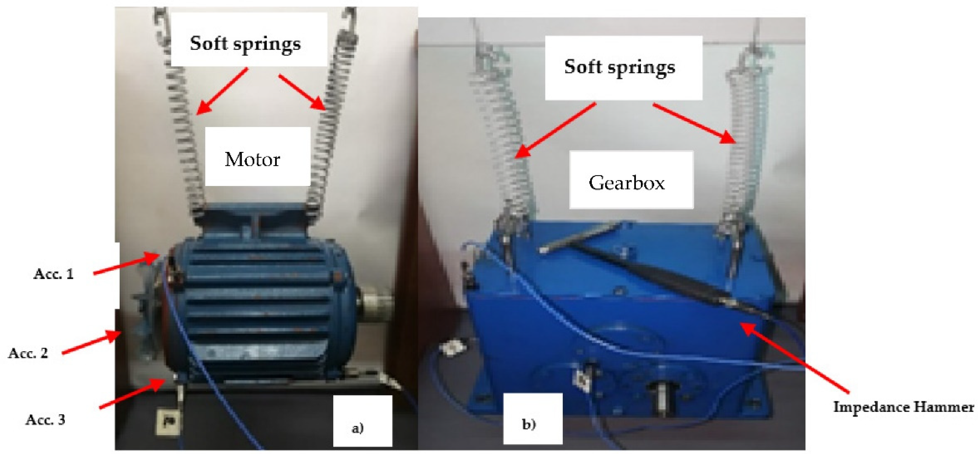
There is considerable growing interest in OMA, due to the modal dynamical properties that can be estimated from the response vibration measurements data. Modal parameters play an important role in structural health monitoring and fault detection. In any case, it will be impossible to apply standard EMA for ambient vibration testing. It is well-known that EMA is carried out under complete machinery shut down. EMA measurement requirements include that the measured object has to be suspended on soft springs to reduce the initial conditions’ effects.

OMA’s major advantages are: the testing procedure can be affordable, cheap, and easy to measure directly on the structure’s surface; testing does not interfere with the machine or structure operation process; the method can be used for large and heavy structures, there is no need for shakers; and there is no need to lift the measurement objects up or hang them up on soft springs.

The OMA also assumes that the structure excitation is on the broadband frequency; however, it can also contain discrete components, such as shaft speed harmonics and gear mesh components. Discrete frequency components can disturb the operation of OMA algorithms. It is quite important to perform a pre-processing of the response signals, in order to remove unwanted excitation components before the application of OMA.

The main objective of our research paper was to determine the structure natural frequencies, based on two of most popular methods, RDT [1,4,11,18] and EITM [3]. The methodology was applied in a steel bar, induction motor, and gearbox. Special attention was paid to closely spaced modes. The CFE and windowing techniques were also applied, similar to what was used in paper [15] to reduce OMA limitations. However, in this case, the liftering technique was used to eliminate the harmonic effects. Different frequency bands were also used as a pre-processing technique to reduce noise. Extensive data tests were performed for the generation of FRFs. The methodology applied in this paper could be an interesting alternative for OMA for health monitoring, fault detection, and machine diagnostics.

5. Conclusions

This paper has sought to highlight the OMA’s properties, in order to determine the structural natural frequencies from vibration signature responses. A new approach was introduced, based on the random decrement technique (RDT), correlation function estimation (CFE), and enhanced Ibrahim time method (EITM), to overcome OMA’s difficulties and limitations. To further reduce the rotational harmonics effects, gear mesh, and side band frequencies, digital signal processing techniques, based on Notching filters and liftering analysis techniques, were used.

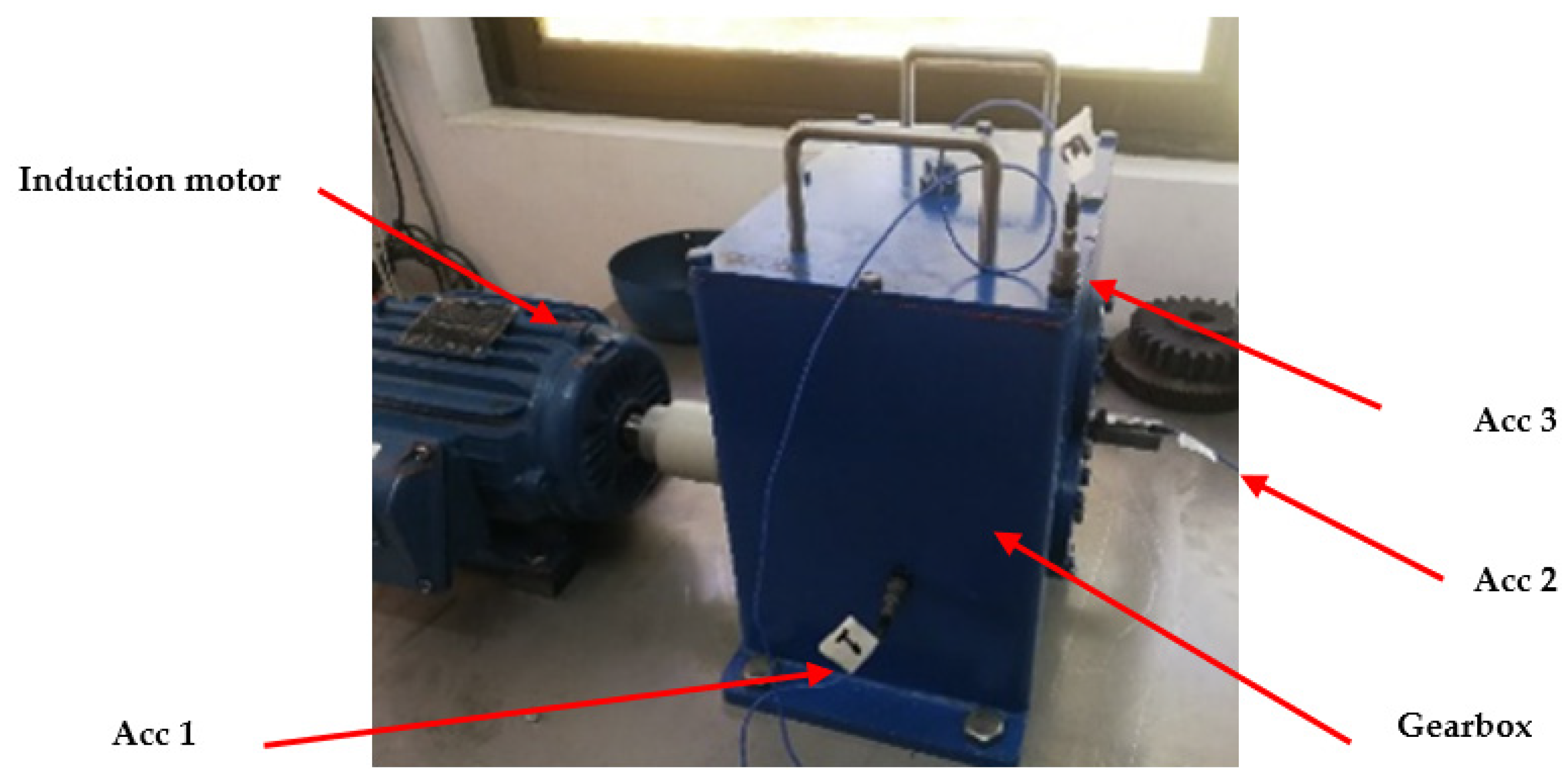
All the experiments were performed at the laboratory test rig and conducted by using three accelerometers, one impedance hammer, one force sensor, and one data acquisition board. To reduce the data’s variabilities, each test was measured three times for 5 min. To validate the proposed methodology, extensive OMA tests were performed for the generation of FRFs. The measured objects were a steel bar, induction motor, and gearbox.

As a final remark, five structural natural frequencies for the induction motor and eight structural natural frequencies for the gearbox were generated, respectively.