
Impact of Lowering Speed Limit on Urban Transportation Network
by
 , , , and
Sunhee Jang
1 ,
,
Seungkook Wu
2,
Daejin Kim
3,
Ki-Han Song
4 ,
,
Seongkwan Mark Lee
5 and
Wonho Suh
1,* 1
Department of Smart City Engineering, Hanyang University ERICA Campus, Ansan 15588, Korea
2
Road Traffic Operation and Pedestrian Mobility Research Team, Korea Transport Institute, Sejong City 30147, Korea
3
Department of Urban Planning & Real Estate, Gangneung-Wonju National University, 7 Jukheon-gil, Gangneung, Gangwon 25457, Korea
4
Department of Civil Engineering, Seoul National University of Science and Technology, 232 Gongneung-ro, Nowon-gu, Seoul 01811, Korea
5
Department of Civil and Environmental Engineering, United Arab Emirates University, Al Ain P.O. Box 15551, United Arab Emirates
*
Author to whom correspondence should be addressed.
Appl. Sci. 2022, 12(11), 5296; https://0-doi-org.brum.beds.ac.uk/10.3390/app12115296
Submission received: 14 April 2022
/
Revised: 12 May 2022
/
Accepted: 20 May 2022
/
Published: 24 May 2022
(This article belongs to the Special Issue Selected Papers from IMETI 2021)
Abstract
:The purpose of this study is to analyze the impact of lowering speed limit on an urban transportation network. A microscopic traffic simulation model, Vissim was utilized to measure the impact. Also, various traffic inputs were tested with different signal coordination scenarios to investigate the impact in different traffic conditions. It was found that during early morning hours with very light traffic, the impact of lowering speed limit was significant. During congested time periods, including level of service E and F, the travel speed reduction from lowering speed limit was not significant. As suggested in other studies, the results demonstrated that lowering the speed limit does not have a significant impact on average travel speed in congested traffic networks. Also, different signal coordination was tested. As expected, signal coordination based on the lowered speed limit performed better than the case with signal coordination based on the previous higher speed limit. The results of this study are expected to provide insights when considering lowering speed limit for existing traffic networks.
1. Introduction
Since April 2021, speed limit lowering policies such as the safety speed 5030 policy have been enforced in South Korea to reduce fatalities and increase traffic safety. The effect of lowering speed limit can be found in other countries from the 1990s: lowering speed limit in urban areas had the effect of reducing the number of deaths by 18.2% in Hungary, and overall accidents in Australia decreased by 23.5% and the number of injuries by 22.3% [1,2]. Several studies have also demonstrated the effect of lowering speed limits resulting in reduced traffic accidents and fatalities [3,4,5,6,7]. However, some local governments and organizations cite lowering speed limits as the main reason for traffic congestion, thereby opposing its introduction. Although studies analyzing the effectiveness of relevant policies by various research institutes suggest that the benefit of lowering speed limits is greater in terms of safety and operational efficiency, there are not enough studies that analyze the impact of policies in various traffic conditions and traffic signal coordination on travel speed.
Additionally, it was believed that lowering speed limit would play a significant impact on vehicle emissions on roadways. However, most of the existing studies utilized the macroscopic model to estimate emissions from vehicles and they applied average speed, not second-by-second individual speed, data to calculate the emission. This macroscopic approach has a limitation in calculating differences in emissions, since it does have the capability of reflecting disaggregated acceleration and deceleration data. It has been reported that vehicle emissions increase in unstable traffic flow conditions including stop-and-go traffic conditions and high acceleration/deceleration traffic conditions. If an average speed is applied in the emission calculation, it is believed to have a greater chance of underestimating vehicle emission, compared to using disaggregate data. Therefore, it is necessary to use microscopic approach utilizing trajectory data of induvial vehicles to realistically calculate the impact on vehicle emission from lowering speed limit. In this study, MOVES OP (operation) mode, a microscopic emission analysis technique, was used to analyze the environmental impact on vehicle emission from lowering speed limit.
The objective of this paper is to investigate the impact on traffic operation and environments from lowering speed limit. Average travel speed and travel time were compared for traffic operational impact analysis, while vehicle emissions were estimated for traffic environmental impact analysis. Various traffic conditions and signal coordination were tested for more comprehensive analysis.
2. Literature Review
The authors found a wide spectrum research on areas related to the impact of lowering speed limit and emission analysis from vehicle speed data. Especially various studies continue to be carried out on the effect of speed management measures on transport network or driver behavior. Some studies investigated the effects of various speed management measures on traffic speed, crash severity, and the transport network altogether. Among them, the authors reviewed relevant studies covering the effect of lowering the speed limit, integration of traffic simulation data with MOVES, and relationship between vehicle speed and emission.
2.1. Studies on the Effect of Lowering the Speed Limit
Lim and Choi evaluated the effect of lowering speed limit in urban areas targeting a total of 29 sections conducted by the Busan Metropolitan Police Agency from 2010 to 2015. As a result of analyzing traffic accident statistics for 1 to 3 years before and after lowering speed limit, the number of traffic accidents decreased by only 3.09% and the number of injuries by only 8.76%, but the number of fatalities decreased by 36.73%, indicating high effectiveness of lowering speed limit in reducing fatalities. In addition, an average travel speed of 6.31 km/h was reduced after lowering speed limit. In most areas, there were statistically significant reductions in average travel speed, confirming the effectiveness of the lowering speed limit policy [8].
Yoon compared travel speed, number of traffic accidents, and number of fatalities in the Seoul metropolitan area. The study showed that by lowering speed limit, traffic accidents on provincial roads decreased [9].
Lee analyzed the effect of lowering speed limit on travel speed and traffic accidents before and after the speed limit change. After lowering speed limit, it was confirmed that the travel speed decreased, and the number of traffic accidents decreased as well [10].
Park evaluated the lowering of speed limit through comparative analysis of the average speed and speed deviation before and after implementing speed limit lowering policy [11]. The results showed that the effect of the policy implementation on average travel speed and standard deviation varied by locations [12,13]. The findings of the previous research are summarized in Table 1.
2.2. Studies on Effects of Speed Limit Reduction or Speed Management Measures on Transport Network or Driver Behavior
Wong and Nicholson conducted an in-depth study of the behavior of drivers negotiating horizontal curves before and after realignment. They found that the path radius could be different from the curve radius, due to substantial variations in lateral placement as vehicles approach and traverse the curves. The study results also showed that contrary to earlier studies, there was not a strong relationship between speed and path radius, but the friction demand does tend to increase as speed increases [14].
Nicholson and Koorey examined the speed profiles of individual vehicles on traffic-calmed streets, in order to provide a better understanding of how drivers react to calming devices over an extended street length and to find ways of estimating speeds along traffic-calmed streets. The results indicated that traffic-calmed streets did not necessarily promote low-speed environments. It was found that 85th percentile speeds at long distances from calming devices were 45–55 km/h for horizontally deflected streets and 40–45 km/h for vertically deflected streets. The study found that drivers had different perceptions of appropriate operating speeds. Also, it was concluded that the most significant factor in determining speeds on streets with vertical deflections was the spacing between devices and the spacing of devices from the street entry [15,16,17].
Nicholson and Koorey investigated the effect of roadway widths for street narrowing with a particular focus on speed and yielding behavior. A 6 m wide two-way pinch-point was found to be not effective in slowing most private vehicles down. The study found that drivers travelled at a similar speed whether they were crossing the pinch-point by themselves or with opposing traffic approaching [18].
2.3. Review Studies on Speed Limit Reduction or Speed Management Measures on Transport Network Safety
Sadeghi-Bazargani and Saadati performed a systematic search on the efficacy/effectiveness of speed control. It was found that speed cameras, engineering planning, intelligent speed adaptation (ISA), speed limits and zones, vehicle activation signs, and integration strategies were the most common strategies reported in the literature. Different strategies had different effects on the average speed of the vehicle in the range of 1.6 to 10 km/h. It has also been reported that the use of different strategies reduced human casualties and fatalities by 8–65% and 11–71%, respectively [3].
Mooren et al. conducted a review based on the recognition that speed management is a pivotal factor in achieving a safer road and traffic system. The study found that speed management, speed limit setting, and infrastructure treatment were effective to enhance safety [4].
Elvik presented a meta-analysis of 33 studies that have evaluated the effects on road safety of area-wide urban traffic calming schemes. The meta-analysis showed that area-wide urban traffic calming schemes on the average reduced the number of injury accidents by about 15%. The largest reduction in the number of accidents was found for residential streets (about 25%) and similar reductions were found in the number of property damage-only accidents [5].
Aarts and Van Schagen reviewed empirical studies regarding driving speed and crashes. It was found that crash rate increased faster with an increase in speed on minor roads than on major roads. Also, speed dispersion was concluded to be an important factor in determining crash rate. Larger differences in speed between vehicles were related to a higher crash rate [6].
Andini et al. conducted a simulation study of speed limit signs and speed markings. The effectiveness of speed management devices was based on the speed reduction according to the speed limit and the comparison of means test analysis. The results of the analysis showed that the most effective speed management device is the speed limit sign by reducing the speed about 4 km/h (7%) [7].
2.4. Studies on Integration of Vissim and MOVES
Xu et al. coupled a Vissim simulation with MOVES to analyze the sensitivity of emissions to simulation parameters in Vissim. They found that the emissions are sensitive to the vehicle type distribution in the fleet, as expected. It was also found that the range of the look-ahead distance in the car-following model and the range of the accepted deceleration rate can impact emissions [19].
Hatem Abou-Senna integrated a micro-traffic simulation model with the latest US Environmental Protection Agency mobile source emissions. Vehicle emissions were estimated based on second-by-second microscopic vehicle operation data. Emissions including CO2 were analyzed from restricted-access highways in micro and stochastic environments [20,21].
Haobing Liu and Daejin Kim analyzed MOVES emission inventory and AERMOD dispersion model based on simulation results. Impacts from different truck operation strategies on PM2.5 emissions and concentrations were investigated [22].
2.5. Studies on the Relationship between Vehicle Speed and Emission
Previous studies confirmed that the relationship between vehicle speed and pollutants generated on the road, such as vehicle exhaust gas, showed a U-shaped curve. Pollutants initially decrease as the vehicle speed increases from zero and then increase again when the vehicle speed surpasses a certain level [23,24].
Lim investigated emission and traffic conditions using the United States emission table. Different level of traffic volumes and intersection signal plans were considered in the analysis. The study suggested that a different strategy is necessary for different traffic conditions [25].
Han reviewed the method of calculating GHG emissions generated by vehicles on highways. GHG emission characteristics were investigated with different traffic environments. It was confirmed that most vehicles except for large trucks emit the lowest GHG emissions at 65–75 km/h [26].
Lee found that acceleration and deceleration have a strong relationship with vehicle emissions. It was demonstrated that the emission was estimated significantly different with different acceleration and deceleration data. It was concluded that the emissions significantly increase as the acceleration increases [27,28,29].
In summary, previous studies investigated the effect of lowering the speed limit in the urban traffic environments, and it was reported that the effect of lowering speed limit varied depending on the traffic conditions. However, there are few studies that investigated the effects of lowering speed limit with respect to various traffic conditions and traffic environments from a perspective of vehicle emission. Therefore, in this study, various traffic conditions including traffic volume and signal offset were investigated using microscopic traffic simulation, and the effect on vehicle emissions from lowering speed limit was investigated.
3. Methodology
3.1. Framework
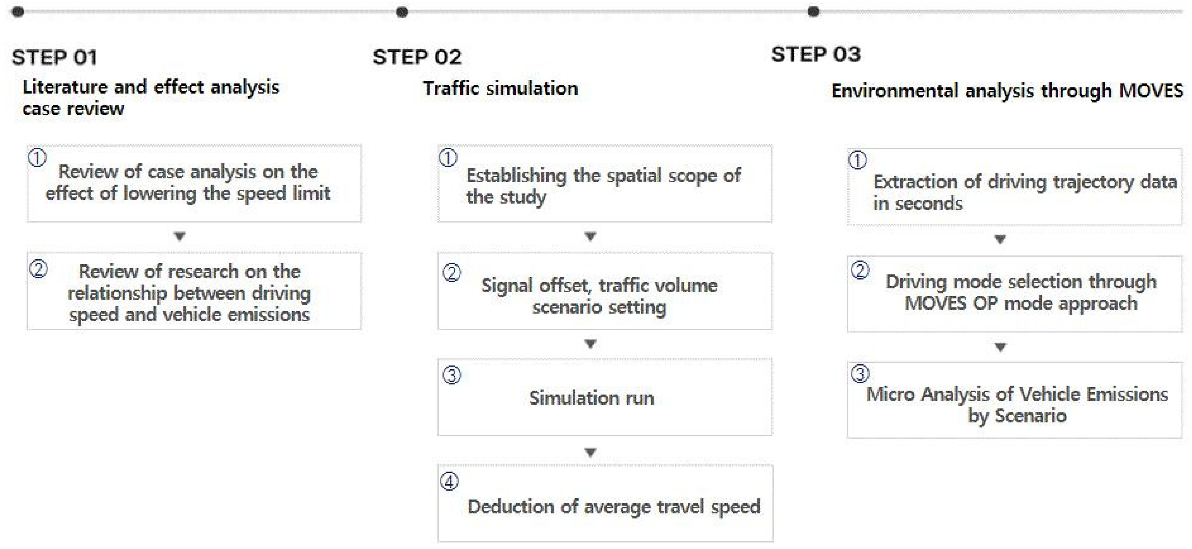
Figure 1 presents the proposed analytical framework in this study. Firstly, previous studies related to the impact analysis of lowering speed limit are reviewed. Also, studies regarding relationship between speed and vehicle emission are assessed. After the review, a traffic simulation model is created, and various traffic volume and offset scenarios are designed. Individual vehicle data including speed, trajectory, and acceleration/deceleration are collected from the simulation. Those data are applied to MOVES OP mode, a microscopic emission analysis technique environmental analysis tool to compare environmental impact from lowering speed limit.
In this study, a microscopic model was used to estimate vehicle emissions. Since the micro model is capable of utilizing second-by-second acceleration and deceleration of individual vehicles, it requires a detailed level of vehicle activity data such as second-by-second vehicle trajectory. The advantage of the micro model is that it can estimate emissions more realistically based on acceleration and deceleration of each vehicle. Using the micro model, it is possible to analyze emissions in stop-and-go traffic conditions and in congested traffic conditions [30].
3.2. MOVES Analysis
As previously mentioned, this study utilized OpModeof MOVES, developed by the U.S. Environmental Protection Agency (EPA). The MOVES OpMode approach uses emission factors according to the vehicle operation mode to classify 23 vehicle operation modes according to the microscopic operating conditions of the vehicle: speed per second, acceleration per second, and vehicle-specific power (VSP) per second. Emissions are calculated by applying emission factors appropriate to the mode (EPA, 2010). As it takes a long time to calculate when multiple vehicle exhaust gases are analyzed using the MOVES tool directly, the MOVES-matrix method is used as an alternative. MOVES-matrix is a model developed by the Georgia Institute of Technology research team which gives the same results as MOVES; its calculation is 200 times faster than the MOVES model. MOVES-Matrix calculates emission factors per unit length and unit time according to road environment, vehicle type, and vehicle age through MOVES, and configures a MOVES-matrix to minimize excessive calculation time that occurs during macroscopic analysis of vehicle exhaust gas [31]. The equation for estimating the emission using the calculated emission factor is calculated as the product of the emission factor, traffic volume, and section length. The micro-emission calculation method proposed in this study is as follows.
- -
- step 1. Micro traffic simulation: extract individual driving trajectory data using VISSIM COM Interface
- -
- step 2. Emission analysis using MOVES OP Mode approach: calculate individual vehicle VSP
To calculate the emission factor using the MOVES OpMode for micro-analysis, it is necessary to calculate the velocity and acceleration of the vehicle trajectory data in seconds as well as the VSP. VSP is calculated as the formula below.
where:
A = rolling resistance coefficient (kW∙s/m),
B = rotational resistance coefficient (kW∙s/m2),
C = aerodynamic drag coefficient (kW∙s3/m3),
m = mass of individual test vehicle (metric tons),
M = fixed mass factor (metric tons),
v = instantaneous vehicle velocity at time t (m/s),
a = instantaneous vehicle acceleration (m/s2),
g = gravitational acceleration (9.8 m/s2), and
u = fractional road grade in percent grade angle (in this study, u = 0)
- -
- step 3. Calculate operation mode ratio by scenario
The VSP (or STP) is assigned to its proper operating mode bins, and the operating mode bins are assigned to emissions and fuel consumption rates stored in MOVES-matrix. To speed up the processing time, the research team prepared a subset of MOVES-matrix for the predefined scenarios. The scenario set is summarized below
- Calendar year: 2018; Month: July,
- Temperature: 80F (average summer temperature in Seoul),
- Humidity: 80% (average summer humidity in Seoul),
- Region: Fulton County, Atlanta (used as a substitute because there is no available MOVES-matrix for Seoul at the time of the analysis; summer weather conditions in Atlanta are similar to those in Seoul), and
- Fuel: default fuel supply and fuel share from MOVES
Descriptions of the operating modes are provided in Figure 2. A MOVES-matrix is prepared for all four running processes, in emission-per-hour by individual source type, model year and operating mode bin (0–40). For each process, VHT (vehicle hours travelled) is calculated from VMT (vehicle miles travelled) and average speed.Then, emissions are estimated by multiplying VHT by source type, model year, and OpMode Bin with corresponding emission rates and then summing emissions by link.
- -
- step 4. Calculate micro-emissions
The last step is to calculate micro-emissions. The operating mode fraction for a single link, vehicle type, and pollutant process is then found according to the following equation [32,33].
where:
FopMode,type,link = (∑TopMode,type,link)/(∑Ttype,link)
F is the operating mode fraction;
T is the collective driving time of all vehicles;
opMode pertains to a specific operating mode;
type pertains to a vehicle type;
link pertains to a “link” or input disaggregation.
3.3. Simulation Network
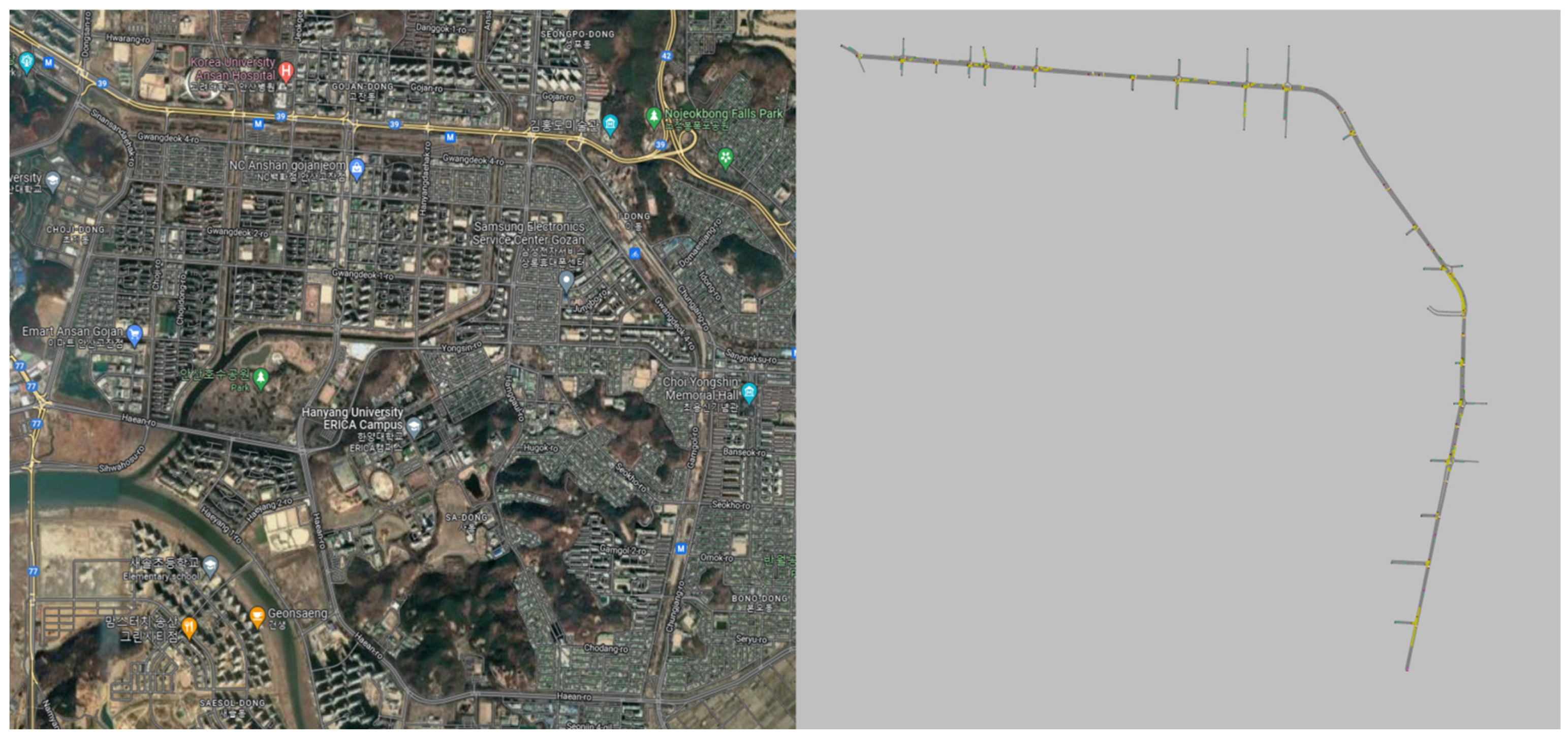
In this study, the spatial range was set to a section about 7.5 km between Gwangdeok 4-ro and Gamgol-ro, Ansan-si. The section to be analyzed starts near Gojan Station on Subway Line 4 which runs alongside the Subway Line 4, passes parallel to Sari Station on the Suin-Bundang Line and meets Haean-ro. The target section is shown in Figure 3.
The analysis target section includes a total of 25 signalized intersections, and the Vissim network was constructed based on the traffic light display data provided by Ansan-si. However, as information on the offset between the signal intersections was not provided, it was calculated through simulation. The vehicle type composition ratio was set as 79% for passenger cars, 3% for heavy vehicles, and 18% for buses based on traffic volume statistics by vehicle type on general national roads. The routing decision was set as 85% for vehicles going straight, 5% for vehicles turning left, and 10% for turning right. In order to reflect a more realistic lane change situation, the starting and finishing points of the entire network were calculated from the starting point of the network, and based on this, the routing decision was set to be decided only at the start of the network. The same setting applies for passenger cars, heavy vehicles, and buses. In addition, the same amount of traffic was set to re-enter from the side street of the intersection as much as the amount of traffic flowing out through left and right turns from the main line using VISSIM COM (python). Through this, the same level of traffic volume was set to be maintained in the entire network section. The list of parameters and their values determined in this research are summarized as follows.
- -
- Simulation resolution: 10
- -
- Average standstill distance: 2 m
- -
- Minimum headway (front/rear): 0.5 m
- -
- Lane change distance: 100 m
- -
- Desired speed range: 47 km/h to 53 km/h for 50 km/h speed limit, and 57 km/h to 63 km/h for 60 km/h speed limit
- -
- Look ahead distance: 0 m (minimum) to 250 m (maximum)
- -
- Look back distance: 0 m (minimum) to 150 m (maximum)
4. Scenario
In this study, traffic volume and signal connection scenarios were established to simulate various traffic conditions using microscopic traffic simulation, and the details are as follows. First, a traffic volume scenario was set. To reflect the actual congested traffic condition, the congestion situation was reproduced by increasing the traffic entering from the side street as well as the amount of traffic entering the network. Depending on the level of service, six traffic volume scenarios were set: 100 vehicles/h, 300 vehicles/h, 500 vehicles/h, 600 vehicles/h, and 600 vehicles/h with side street traffic increased by 30%, and 600 vehicles/h with side street traffic increased by 50%. Next, a signal connection scenario was set. A continuous progression interlocking system was used to set the signal offset. The formula for calculating the offset in a continuous system is as follows.
T = Ideal signal offset (s),
l = Link length, distance between intersections (m),
v = vehicle speed (m/s),
It was assumed that the offset was set to maximize the overall travel speed, and the process of determining the offset setting value was performed through simulation. As a result, the offset was set as the time required for a vehicle going straight at the speed limit to pass between each intersection. Table 2 and Table 3 show the speed limit and offset scenarios and traffic input scenarios, respectively.
5. Result
5.1. Vissim Simulation Results
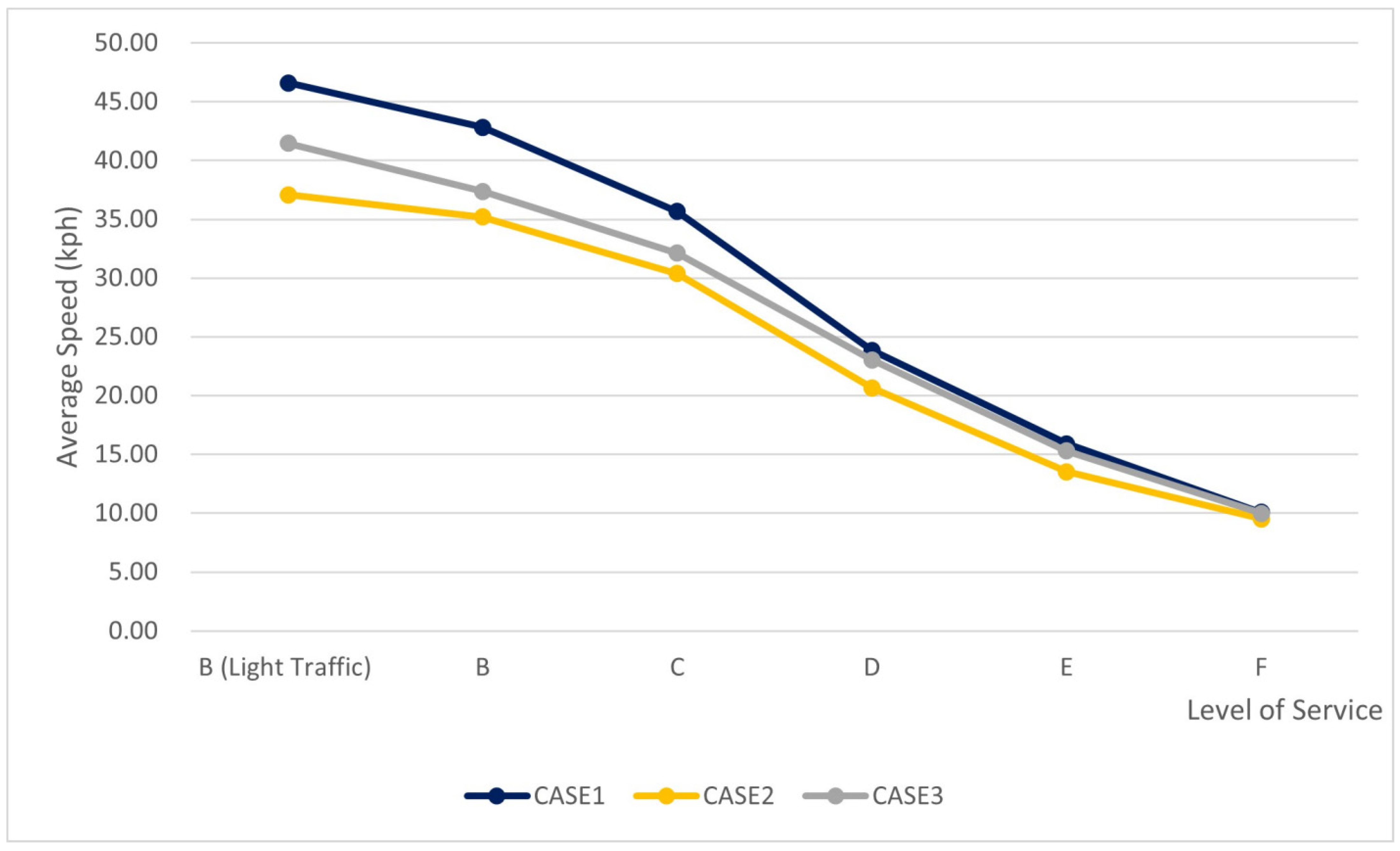
Ten replicated runs with different random seed numbers were conducted in this study. Table 4 and Figure 4 show the average speed results from the replicated runs. As a result of comparing the average traffic speed by scenario, average traffic speed of CASE 1 was analyzed to maintain 40 km/h or more in a light traffic condition of the level of service B. In the same traffic situation, CASE 2 and CASE 3 were found to maintain an average traffic speed of 35 km/h or more. In addition, CASE 3 showed a traffic speed of a maximum of 4 km/h higher than that of CASE 2. This implies that in a light traffic condition of the level of service B, CASE 1 with a high-speed limit shows the smoothest traffic followed by CASE 3.
As traffic volume increases above 500 veh/h/ln, the level of service deteriorated from B to C in CASE 1, but the speed difference by CASE became smaller. In addition, it was derived that the traffic speed of CASE 3 was higher than that of CASE 2 by 2 km/h. When the traffic volume in the side street was increased at a traffic volume of 600 veh/h/ln, the level of service was deteriorated from D to E or F based on CASE 1. CASE 2 and CASE 3 also showed a deteriorated service level as the traffic volume increased. When comparing the same input traffic volume, it was analyzed that the difference in the average traffic speed of CASE 1, CASE 2, and CASE 3 at the level of service E was within 2 km/h.
At the level of service F, the difference in traffic speed of CASE 1, CASE 2, and CASE 3 was around 1 km/h. The changing trend of the average traffic speed for each scenario according to traffic volume can be seen in Figure 2. As shown in the figure, when the traffic situation is smooth, the average traffic speed is relatively high in CASE 1 compared to CASE 2 and CASE 3. As the level of service deteriorates, the gap narrows down gradually; at the level of service F, it can be seen that the gap between CASE 1, CASE 2, and CASE 3 is relatively small.
To find out whether there is a difference in the average travel speed under different offset data with the same speed limit, t-test analysis was conducted. In most of traffic conditions, it was found that there was a significant difference under the level of 0.05 significance. However, the significance level was 0.609 in the level of service, F, indicating that there was no significant difference. It was an expected outcome, since the impact of different offsets in signal coordination is minimal in congested traffic conditions. The results of the t-test are provided in Table 5.
5.2. Total Emissions per Vehicle
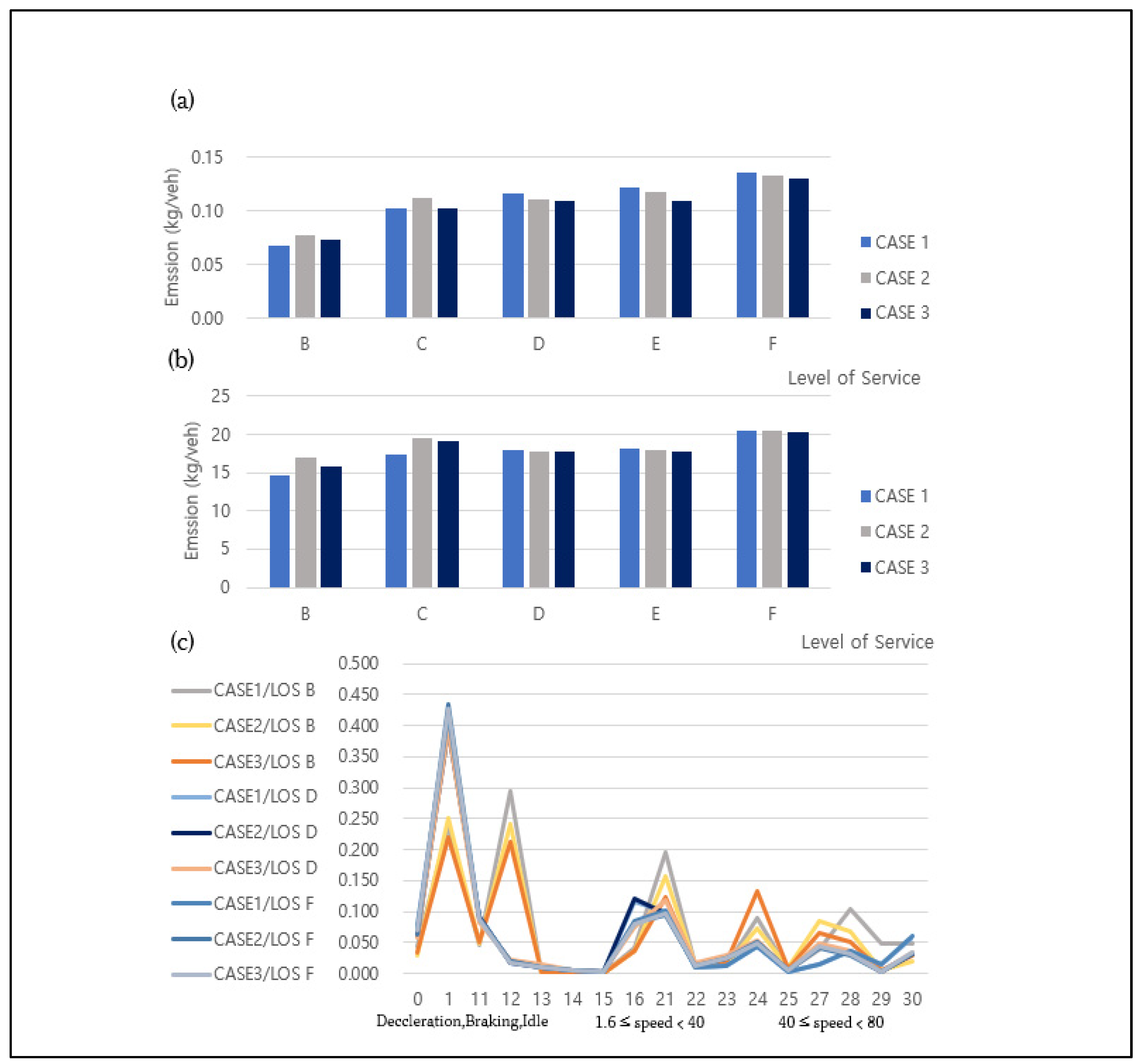
Next, the CO2 and NOx emissions per vehicle were analyzed using the MOVES OP mode approach. The results are shown in Figure 5, Table 6 and Table 7. The analysis shows the least vehicle emission gases when the speed limit is 60 km/h at the levels of service B and C. As for CASE 2, CO2 increased up to 15.5% and NOx up to 12.9%. As for CASE 3, CO2 increased up to 8.3% and NOx increased up to about 7.5%.
At the levels of service E and F, the emission of CASE 1 was the largest, and in CASE 2, 0.07% less CO2 and 1.97% less NOx were generated. In CASE 3, it was confirmed that CO2 decreased by 0.89% and NOx decreased by about 3.87%. Through this, it was confirmed that the emission gases were generated in a similar level or decreased after lowering speed limit at the levels of service D, E, and F.
6. Conclusions
This study analyzed the impact of lowering speed limit on traffic network under different traffic inputs and signal offsets using microscopic traffic simulation on the operational and environmental perspective. As a result of analyzing the average traffic speed using microscopic traffic simulation, at times with less vehicle volume, the difference in traffic speed before and after lowering speed limit was relatively large at 5 km/h, but at times with heavy vehicle volume or congestion (levels of service E and F), the difference in traffic speed was less than 1 km/h, indicating that lowering speed limit has almost no impact on the average traffic speed. In addition, where the speed limit is the same, there was up to 5 km/h difference in traffic speed according to the offset. CO2 and NOx emissions were also analyzed using the MOVES OP mode approach. As a result, at the levels of service B and C, the emissions were the lowest when the speed limit was 60 km/h, and after lowering speed limit, it was confirmed that the emissions increased up to 15%. However, at times with heavy traffic volume or congestion, the vehicle emission gas generation was the largest when the speed limit was 60 km/h, and it was confirmed that after lowering speed limit, the emissions decreased up to 4%.
The findings from this study are compatible with the findings from previous studies. For example, Lim and Choi analyzed the effect of lowering the speed limit on the average travel speed using travel speed data in Busan, South Korea. They found that the average driving speed decreased by 6.31 km [8]. Yoon analyzed the effect of lowering the speed limit on the average traveling speed of urban roads. It was found that the average traveling speed decreased by 2 km/h from 42.4 km/h to 40.3 km/h [9]. Also, Park analyzed the average speed and standard deviation according to the speed limit using driving record data and confirmed the effect of reducing the average speed [10]. As Park suggested, the effect of lowering speed limit varies location to location. This study confirms its variation depending on the location and traffic conditions with creating different traffic conditions with various vehicle inputs and signal coordination parameters. Additionally, previous studies mainly focused on speed reduction and environmental impacts were not considered in the analysis. In this study, environmental impacts were analyzed with various traffic conditions.
As other studies pointed out, it is difficult to draw a generalized conclusion of lowering speed limit policy since many variables are involved in traffic conditions. This study conducted more comprehensive analysis including different traffic conditions with low-volume traffic to congested traffic with different signal coordination parameters. Additionally, environmental impact was considered in this paper. Therefore, it is hoped that this paper provides a better insight to transportation planners and policy makers when considering lowering speed limit for existing traffic networks. The limitations of this study are as follows. First, in this study, analysis was performed using simulation to reflect various traffic conditions. In order to accurately analyze the effect of the speed-limit-lowering policy, it is judged that it is necessary to analyze the actual driving data before and after the speed-limit-lowering. Second, information on the current signal intersection can be confirmed as public data, but information on the offset between the signal intersections is not provided. Therefore, in this study, a simulation was used to calculate the optimal offset. To calculate a more appropriate offset, it is judged that additional research is needed on the interlocking technique for calculating the optimal offset. Third, in this study, the factors affecting the speed limit were assumed to be signal offset and traffic volume. It is judged that it is necessary to conduct additional research in consideration of factors affecting the speed limit, such as intersection spacing, signal control conditions, traffic volume, lane width, and traffic friction factors. In this study, an analysis of the impact of the speed-limit-lowering policy was conducted, focusing on traffic speed and exhaust gas, which are of high interest to the public. The results of this study are expected to be used as reference data for the establishment and ex post evaluation of strategies for expanding the speed limit lowering policy through additional research that reflects actual traffic conditions in the future.
Author Contributions
W.S. and S.W. conceived of the presented idea. S.J. and D.K. developed the theory and performed the computations. S.J. carried out the simulation. W.S. and S.J. wrote the manuscript in consultation with S.W., S.M.L., K.-H.S. and S.M.L. contributed to the interpretation of the results. All authors discussed the results and contributed to the final manuscript. All authors have read and agreed to the published version of the manuscript.
Funding
This work was partially supported by NRF-2020R1A2C1011060 of the Korean government.
Institutional Review Board Statement
Not applicable.
Informed Consent Statement
Not applicable.
Data Availability Statement
The data presented in this study are available on request.
Conflicts of Interest
The authors declare no conflict of interest.
References
- Sugiyanto, G.; Jajang; Santi, M. The impact of lowering speed limit on mobility and the environment. AIP Conf. Proc. 2019, 2094, 020019. [Google Scholar] [CrossRef]
- Austroads. Urban Speed Management in Australia AP, 118-96, New South Wales. 1996. Available online: https://austroads.com.au/publications/road-safety/ap-118-96 (accessed on 1 February 2022).
- Sadeghi-Bazargani, H.; Saadati, M. Speed Management Strategies, A Systematic Review. Bull. Emerg. Trauma 2016, 4, 126–133. [Google Scholar]
- Mooren, L.; Shuey, R.; Hamelmann, C.; Mehryari, F.; Abdous, H.; Haddadi, M.; Hosseinizadeh, S. Road safety case studies: Speed management in Iran: A review process. J. Road Saf. 2021, 32, 31–42. [Google Scholar] [CrossRef]
- Elvik, R. Area-wide urban traffic calming schemes: A meta-analysis of safety effects. Accid. Anal. Prev. 2001, 33, 327–336. [Google Scholar] [CrossRef]
- Aarts, L.; van Schagen, I. Driving speed and the risk of road crashes: A review. Accid. Anal. Prev. 2006, 38, 215–224. [Google Scholar] [CrossRef]
- Andini, F.; Kusumastutie, N.; Purwanto, E.; Rusmandani, P.; Yusup, L. The effectiveness of speed limit sign and marking as the speed management devices. Adv. Eng. Res. 2020, 193, 139–142. [Google Scholar] [CrossRef] [Green Version]
- Lim, C.; Choi, Y. Study of Downward Speed Limit of Main Roads on Traffic Accident and Effect Analysis—In Busan Metropolitan City. KSCE J. Civ. Environ. Eng. Res. 2018, 38, 81–90. [Google Scholar] [CrossRef]
- Yoon, Y. A Comparative Study on the Traffic Effects of Speed Limit Reduction on the Urban and Provincial Roads. J. Korea Contents Assoc. 2020, 20, 430–438. [Google Scholar] [CrossRef]
- Lee, W.; Seong, N.; Park, G. Analysis of Regulatory Speed Limit and Its’ Effect. J. Korean Soc. Saf. Educ. 2002, 5, 5–16. [Google Scholar]
- Park, S.; Suh, W. Effectiveness Evaluation of the Safe Speed 5030 Polity; Korea Transportation Safety Authority Report; Korea Transportation Safety Authority: Gimcheon, Korea, 2020. [Google Scholar]
- Lee, H.; Jung, H. A Study on the Factors Affecting the Acceptance of the Safety Speed 5030 Policy. KSCE J. Civ. Environ. Eng. Res. 2021, 41, 559–569. [Google Scholar] [CrossRef]
- Lee, N. Traffic Accident Effectiveness Analysis of changing Regulatory Speed Limit. Master’s Thesis, University of Seoul, Seoul, Korea, 2007. [Google Scholar]
- Wong, Y.; Nicholson, A. Speed and lateral placement on horizontal curves. Road Transp. Res. 1993, 2, 74–87. [Google Scholar]
- Daniel, B.; Nicholson, A.; Koorey, G. Investigating speed patterns and estimating speed on traffic-calmed streets. In Proceedings of the IPENZ Transportation Group Conference Auckland, Auckland, New Zealand, 27–30 March 2011. [Google Scholar]
- Daniel, B.; Nicholson, A.; Koorey, G. Analysing speed profiles for the estimation of speed on traffic-calmed streets. Road Transp. Res. 2011, 20, 57–70. [Google Scholar] [CrossRef]
- Daniel, B.; Nicholson, A.; Koorey, G. The effects of vertical speed control devices on vehicle speed and noise emission. In Proceedings of the 25th ARRB Conference, Perth, Australia, 23–26 September 2012. [Google Scholar]
- Chai, C.; Koorey, G.; Nicholson, A. The effectiveness of two-way street calming pinch-points. In Proceedings of the Institution of Professional Engineers New Zealand (IPENZ) Transportation Conference, Auckland, New Zealand, 27–30 March 2011. Corpus ID: 06642193. [Google Scholar]
- Xu, X.; Liu, H.; James, M. Estimating Project-Level Vehicle Emissions with Vissim and MOVES-Matrix. Transp. Res. Rec. 2016, 2570, 107–117. [Google Scholar] [CrossRef] [Green Version]
- Abou-Senna, H. Microscopic Assessment of Transportation Emissions on Limited Access Highways. Ph.D. Thesis, University of Central Florida, Orlando, FL, USA, 2012; p. 2461, CFE0004777. [Google Scholar]
- Abou-Senna, H.; Radwan, E. VISSIM/MOVES integration to investigate the effect of major key parameters on CO2 emissions. Transp. Res. Part D Transp. Environ. 2013, 21, 39–46. [Google Scholar] [CrossRef]
- Liu, H.; Kim, D. Simulating the uncertain environmental impact of freight truck shifting programs. Atmos. Environ. 2019, 214, 116847. [Google Scholar] [CrossRef]
- Ziemska, M. Exhaust Emissions and Fuel Consumption Analysis on the Example of an Increasing Number of HGVs in the Port City. Sustainability 2021, 13, 7428. [Google Scholar] [CrossRef]
- Guensler, R.; Liu, H.; Xu, Y. Energy Consumption and Emissions Modeling of Individual Vehicles. Transp. Res. Rec. 2017, 2627, 93–102. [Google Scholar] [CrossRef]
- Park, J.; Jung, S.; Lim, K. The study on the reduction of vehicle emission using optimal signal strategy on intersection. Proc. KOR-KST Conf. 2005, 48, 357–364. [Google Scholar]
- Han, D.; Hong, S.; Lee, S. Development of CO₂ Emission Estimating Methodology of Electronic Toll Collection System Based on Instantaneous Speed and Acceleration. J. Transp. Res. 2012, 19, 63–76. [Google Scholar] [CrossRef]
- Lee, Y.; Cho, H.; Park, J. A Study on the Estimation Method for Emission from Vehicles Considering Individual Driving Behaviors. Seoul Stud. 2004, 5, 43–59. [Google Scholar]
- Lee, Y. A Study of Calculation Methodology of Vehicle Emissions based on Driver Speed and Acceleration Behavior. J. Korean Soc. Transp. 2011, 29, 107–120. [Google Scholar]
- Chauhan, B.; Joshi, G.; Parida, P. Speed Trajectory of Vehicles in VISSIM to Recognize Zone of Influence for Urban-Signalized Intersection; Lecture Notes in Civil Engineering; Springer: Singapore, 2020; p. 69. [Google Scholar] [CrossRef]
- Saroj, A.; Roy, S.; Guin, A.; Hunter, M.; Fujimoto, R. Smart City Real-time Data-driven Transportation Simulation. In Proceedings of the 2018 Winter Simulation Conference (WSC), Gothenburg, Sweden, 9–12 December 2018; pp. 857–868. [Google Scholar] [CrossRef]
- Kim, D.; Ko, J.; Xu, X.; Liu, H.; Rodgers, M.; Guensler, R. Evaluating the Environmental Benefits of Median Bus Lanes: Microscopic Simulation Approach. Transp. Res. Rec. 2019, 2673, 663–673. [Google Scholar] [CrossRef]
- Liu, A. Real-Time Vehicle Emission Estimation Using Traffic Data. UW Space. 2019. Available online: http://hdl.handle.net/10012/14680 (accessed on 1 February 2022).
- Abdel-Aty, M.; Dilmore, J.; Dhindsa, A. Evaluation of variable speed limits for real-time freeway safety improvement. Accid. Anal. Prev. 2006, 38, 335–345. [Google Scholar] [CrossRef] [PubMed]
Figure 1.
Study procedure.

Figure 2.
Operating mode descriptions.

Figure 3.
Simulation Network.

Figure 4.
Average speed comparison.

Figure 5.
Emission comparison: (a) NOx, (b) CO2, and (c) operating mode bin distributions by scenario.
Figure 5.
Emission comparison: (a) NOx, (b) CO2, and (c) operating mode bin distributions by scenario.


Table 1.
Summary of previous research.
| Authors | Findings after Lowering Speed Limit |
|---|---|
| Lim and Choi (2018) | Average 6.31 km/h decrease |
| Yoon (2020) | 4.9% (urban roads) and 4.6% (rural roads) of speed decrease |
| Lee (2007) Park (2020) | Reduction in traffic volume, speed, and traffic accidents Reduction in average speed |
Table 2.
Speed limit and offset scenarios.
| Case No. | Speed Limit | Offset |
|---|---|---|
| CASE 1 | 60 km/h | Offset to obtain highest average travel speed at 60 km/h speed limit |
| CASE 2 | 50 km/h | Offset to obtain highest average travel speed at 60 km/h speed limit |
| CASE 3 | 50 km/h | Offset to obtain highest average travel speed at 50 km/h speed limit |
Table 3.
Traffic input scenarios.
| Level of Service | B with Light Traffic | B | C | D | E | F |
|---|---|---|---|---|---|---|
| Traffic Input (veh/h/ln) | 100 | 300 | 500 | 600 | 600 with side street traffic 30% increase | 600 with side street traffic 50% increase |
Table 4.
Average travel speed (km/h).
| Level of Service | B with Light Traffic | B | C | D | E | F |
|---|---|---|---|---|---|---|
| CASE 1 | 46.60 | 42.83 | 35.65 | 23.84 | 15.89 | 10.08 |
| CASE 2 | 37.08 | 35.21 | 30.39 | 20.67 | 13.53 | 9.52 |
| CASE 3 | 41.46 | 37.37 | 32.11 | 23.05 | 15.29 | 9.99 |
Table 5.
Statistical results.
| Level of Service | Case | Mean | Std. Deviation | t | Sig. |
|---|---|---|---|---|---|
| B with light traffic | Case 2 Case 3 | 37.08 41.46 | 0.51 0.88 | −14.54 | 0.000 |
| B | Case 2 Case 3 | 35.21 37.37 | 0.22 0.74 | −7.67 | 0.000 |
| C | Case 2 Case 3 | 30.38 32.11 | 0.44 0.54 | −4.62 | 0.000 |
| D | Case 2 Case 3 | 20.67 23.05 | 1.24 1.26 | −2.01 | 0.048 |
| E | Case 2 Case 3 | 13.56 15.28 | 0.58 0.63 | −5.95 | 0.000 |
| F | Case 2 Case 3 | 9.52 9.99 | 0.27 0.39 | 0.52 | 0.609 |
Table 6.
CO2 emission (kg/veh).
| Level of Service | B | C | D | E | F |
|---|---|---|---|---|---|
| CASE 1 | 14.62 | 17.41 | 17.91 | 18.21 | 20.53 |
| CASE 2 | 16.88 | 19.43 | 17.79 | 17.92 | 20.52 |
| CASE 3 | 15.83 | 19.07 | 17.69 | 17.80 | 20.35 |
Table 7.
NOx emission (g/veh).
| Level of Service | B | C | D | E | F |
|---|---|---|---|---|---|
| CASE 1 | 68 | 103 | 117 | 122 | 136 |
| CASE 2 | 77 | 112 | 111 | 118 | 133 |
| CASE 3 | 73 | 103 | 109 | 110 | 130 |
Publisher’s Note: MDPI stays neutral with regard to jurisdictional claims in published maps and institutional affiliations. |
© 2022 by the authors. Licensee MDPI, Basel, Switzerland. This article is an open access article distributed under the terms and conditions of the Creative Commons Attribution (CC BY) license (https://creativecommons.org/licenses/by/4.0/).
Share and Cite
MDPI and ACS Style
Jang, S.; Wu, S.; Kim, D.; Song, K.-H.; Lee, S.M.; Suh, W. Impact of Lowering Speed Limit on Urban Transportation Network. Appl. Sci. 2022, 12, 5296. https://0-doi-org.brum.beds.ac.uk/10.3390/app12115296
AMA Style
Jang S, Wu S, Kim D, Song K-H, Lee SM, Suh W. Impact of Lowering Speed Limit on Urban Transportation Network. Applied Sciences. 2022; 12(11):5296. https://0-doi-org.brum.beds.ac.uk/10.3390/app12115296
Chicago/Turabian StyleJang, Sunhee, Seungkook Wu, Daejin Kim, Ki-Han Song, Seongkwan Mark Lee, and Wonho Suh. 2022. "Impact of Lowering Speed Limit on Urban Transportation Network" Applied Sciences 12, no. 11: 5296. https://0-doi-org.brum.beds.ac.uk/10.3390/app12115296
Note that from the first issue of 2016, this journal uses article numbers instead of page numbers. See further details here.