Intelligent Computer-Aided Model for Efficient Diagnosis of Digital Breast Tomosynthesis 3D Imaging Using Deep Learning

Abstract

Digital breast tomosynthesis (DBT) is a highly promising 3D imaging modality for breast diagnosis. Tissue overlapping is a challenge with traditional 2D mammograms; however, since digital breast tomosynthesis can obtain three-dimensional images, tissue overlapping is reduced, making it easier for radiologists to detect abnormalities and resulting in improved and more accurate diagnosis. In this study, a new computer-aided multi-class diagnosis system is proposed that integrates DBT augmentation and colour feature map with a modified deep learning architecture (Mod_AlexNet). To the proposed modified deep learning architecture (Mod AlexNet), an optimization layer with multiple high performing optimizers is incorporated so that it can be evaluated and optimised using various optimization techniques. Two experimental scenarios are applied, the first scenario proposed a computer-aided diagnosis (CAD) model that integrated DBT augmentation, image enhancement techniques and colour feature mapping with six deep learning models for feature extraction, including ResNet-18, AlexNet, GoogleNet, MobileNetV2, VGG-16 and DenseNet-201, to efficiently classify DBT slices. The second scenario compared the performance of the newly proposed Mod_AlexNet architecture and traditional AlexNet, using several optimization techniques and different evaluation performance metrics were computed. The optimization techniques included adaptive moment estimation (Adam), root mean squared propagation (RMSProp), and stochastic gradient descent with momentum (SGDM), for different batch sizes, including 32, 64 and 512. Experiments have been conducted on a large benchmark dataset of breast tomography scans. The performance of the first scenario was compared in terms of accuracy, precision, sensitivity, specificity, runtime, and f1-score. While in the second scenario, performance was compared in terms of training accuracy, training loss, and test accuracy. In the first scenario, results demonstrated that AlexNet reported improvement rates of 1.69%, 5.13%, 6.13%, 4.79% and 1.6%, compared to ResNet-18, MobileNetV2, GoogleNet, DenseNet-201 and VGG16, respectively. Experimental analysis with different optimization techniques and batch sizes demonstrated that the proposed Mod_AlexNet architecture outperformed AlexNet in terms of test accuracy with improvement rates of 3.23%, 1.79% and 1.34% when compared using SGDM, Adam, and RMSProp optimizers, respectively.

1. Introduction

Breast cancer is a significant global health issue and one of the leading causes of mortality amongst women. The World Health Organization (WHO) reported that in 2020, there were 2.3 million women diagnosed with breast cancer and 685,000 deaths globally. Breast cancer has been detected in 7.8 million women worldwide between 2015 and 2021, making it the most common cancer in the world [1]. About one in eight women (about 12%) in the UK are diagnosed with breast cancer during their lifetime [2]. Early detection and diagnosis are critical for treatment, recovery, and lowering mortality rates. Based on the stage of cancer, the survival rate and prognosis differ significantly. The sooner cancer is identified, the more effective the treatment will be [3].

Digital breast tomosynthesis is a revolutionary three-dimensional imaging scan for the breast that intends to improve abnormality detection [4]. The 3D model is constructed using digital breast tomosynthesis, which reconstructs numerous projections of low-dose pictures produced by a digital X-ray source moving over a limited arc angle [5]. When compared to mammography, the DBT allows the lesion to be segregated from the breast tissue background, resulting in improved detectability, thus overcoming the tissue overlapping challenge that faces traditional mammography [6].

Computer-aided diagnosis (CAD) tools are already being utilised to aid radiologists in their decision-making. Such technologies could considerably reduce the amount of time and effort required to assess a lesion in clinical practice, while also reducing the number of false positives that result in needless and uncomfortable biopsies [7]. Deep learning is a recent technological innovation that has outperformed the state-of-the-art in a variety of machine learning tasks, including object identification and classification. Deep learning approaches adaptively train the proper feature extraction procedure from the input data for the target output, unlike traditional machine learning methods, which require a hand-crafted feature extraction stage, which is challenging because it relies on a knowledge base [7].

Deep learning (DL) and convolutional neural networks (CNNs) have been employed to segment, classify, and detect breast tumours in a variety of research in recent years. For automatic detection of speculated mass, Yousefi, Mina et al. [8] proposed three distinct CAD frameworks: hand-crafted, feature-based MIL framework, DCNN multiple instance-random forest (DCNN MI-RF), and deep cardinality-restricted Boltzmann machine multiple instance-random forest (DCaRBM MI-RF). Pre-processing of all DBT slices included data augmentation, noise removal, and slice removal of the pectoral muscle. Three classifiers, multiple-instance random forest (MI-RF), multiple-instance support vector machine (MISVM), and multiple-instance semi-supervised support vector machine (MissSVM), were implemented to compare the three frameworks. Classification of the DCNN framework using the MI-RF yielded the best performance with an 86.81% accuracy, 87.5% specificity, and 86.6% sensitivity.

Bevilacqua, Vitoantonio et al. [9] developed two frameworks, one that used artificial neural networks (ANN) and the other that used several deep learning models. All DBT slices were pre-processed and segmented, which included contrast enhancement, border removal, and lesion segmentation if one was discovered. The first framework extracted features using a gray-level co-occurrence matrix (GLCM), followed by a developed ANN. The second framework extracted the features using seven different DL models and the classification was performed by SVM, k-nearest neighbours (KNN), Naïve Bayes (NB), linear discriminant analysis (LDA) and decision tree (DT). The first framework observed an accuracy of 84.19%, whereas the second framework had an accuracy of 92.02% on a 2-class classification.

Samala, Ravi et al. [10] developed a multi-stage transfer learning model. In the first stage, 9623 augmented ROIs from 2454 mass lesions on mammograms were used to train a pre-trained DCNN on ImageNet. The second stage deployed a DCNN for feature extraction followed by feature selection and random forest classifier. Pathway evolution was carried out iteratively using the genetic algorithm (GA), with tournament selection based on court-preserving crossover and mutation. Using leave-one-case-out cross-validation, the second stage was trained on 9120 DBT ROIs from 228 mass lesions. The 2-class classification resulted in an 0.90 area under the ROC curve (AUC).

In Hassan, Loay et al. [11], demonstrated fully automated deep-learning approaches for detecting breast lesions on a publicly available dataset. They looked at how well two data augmentation strategies (channel replication and channel concatenation) worked with five cutting-edge deep learning detection models. The implemented DL models were YOLO-Small (S), YOLOMedium (M), YOLO-Large (L), YOLO-XLarge (XL), and Faster R-CNN.

This paper proposes a computer-aided multi-class diagnosis system for classifying DBT scans as benign, malignant, or normal. DBT augmentation techniques and colour mapping are integrated with a modified deep learning architecture (Mod_AlexNet) in the multi-class diagnosis model. An optimization layer with multiple high performing optimizers is added to the proposed modified deep learning architecture (Mod_AlexNet) so that it can be analysed and optimised using optimization algorithms.

This research highlights some of the key deep learning models as well as a newly proposed modified deep learning architecture (Mod_AlexNet). To efficiently classify DBT slices, two experimental scenarios are applied. The first scenario proposed a computer-aided diagnosis (CAD) model that integrated DBT augmentation, image enhancement techniques, and colour feature mapping with six deep learning models for feature extraction, including ResNet-18, AlexNet, GoogleNet, MobileNetV2, VGG-16, and DenseNet-201. The features were then classified using a support vector machine (SVM) classifier. The second scenario used several optimization techniques to compare the performance of the newly proposed Mod_AlexNet architecture and traditional AlexNet, and different evaluation performance metrics were computed. For different batch sizes, the optimization techniques included adaptive moment estimation (Adam), root mean squared propagation (RMSProp), and stochastic gradient descent with momentum (SGDM).

This paper is organised into five sections. Section 2 contains the proposed model’s architecture, deep learning models that have been implemented, and a detailed description of each phase. Section 2 also includes a description of the dataset, the experimental setup, and the performance measures. Section 3 shows and compares the results of the two experimental scenarios. Section 4 presents a discussion of the proposed model and its results. Finally, in Section 5, conclusions are drawn.

2. Materials and Methods

2.1. Proposed Model

The proposed model was implemented to classify DBT slices into normal, benign, or malignant. To construct the model, various image processing algorithms were implemented and shown in Figure 1.

2.1.1. Data Augmentation

Data augmentation is a method of intentionally increasing the volume and complexity of existing data. In recent years, data augmentation has been a popular research topic in the field of deep learning. Neural networks require a large number of training samples in deep learning; yet, existing datasets in the medical area have low resources. To expand the diversity of the original dataset, a data augmentation step is required [12].

The most well-known methods:

• Flipping: makes a mirror replica of the original image.
• Rotation: rotating an image around the centre pixel.
• Saturation: changing the separation between colours of an image.
• Value: changes the relative lightness or darkness of a colour.
• Hue: the process of changing the shade of the colours in an image.
• Adding Noise: addition of noise to the image.

In the proposed model, at first, images were flipped, afterwards, randomly selected values were applied for the brightness in the range [−0.3,−0.1], saturation in the range [−0.4,0.2], and hue in the range [0.05,0.25]. Figure 2 shows a visualization of different applied augmentation techniques. The original image was flipped in Aug1 and Aug2, and random saturation and hue values were applied in Aug1. Brightness and hue values were chosen at random for Aug2. Aug3 and Aug4 applied randomly selected saturation and brightness values to the original image, whereas Aug4 additionally applied random selection of hue values.

In this study, each tomosynthesis slice produced four augmented images. Two images have been flipped, while the other two have not been flipped. Following that, contrast limited adaptive histogram equalisation (CLAHE) was applied to improve the image’s local contrast along with random brightness, saturation, and hue values. In the training set, scans from 480 patients were included of which 400 normal patients (total of 96,862 slices), 50 patients with benign findings (total of 7034 slices), and 30 patients with malignant findings (total of 4242 slices). The augmentation was carried out as the first stage for slice preparation for the training set. The total number of training slices after augmentation is 387,448 normal slices, 28,136 benign slices, and 16,968 malignant slices.

2.1.2. Pre-Processing

The pre-processing stage consists of multiple phases. The first phase is slicing the DBT volume into 2D slices. The second stage aims to enhance the DBT slices through noise suppression, edge enhancement, and contrast enhancement using different filters and morphological operations.

2.1.3. Colour Feature Map

After enhancing the image’s contrast and edges, additional modifications are required to remove any background noise that may be present. The steps are as follows:

• Background Artefact Removal

Background artefacts and labels affect the model’s accuracy since they may give false indications when extracting the features from the image. Low-level artefacts, labels, high-level artefacts, and background noises are examples of background artefacts. To distinguish the foreground from the background, the image was first transformed from grayscale to a binary format. Second, to eliminate salt noise from the image, an opening morphological technique is used. Finally, little white patches were deleted, and the binary mask’s biggest area was chosen, suppressing all artefacts and labels detected in the mammography.

2.

Colour Map Application

To distinguish between distinct parts in the image, the colour map was applied in HSV colours. Colours in different locations have varied hues, saturations, and values. Figure 3 shows how different colour intensities correspond to different clusters that translate to different mammography classes and findings. Finally, the slices are resized to match the input size for each DL model.

2.1.4. Deep Convolution Neural Networks

The process of transferring the weights of a pre-trained CNN model is called transfer learning. It is the process of moving the weights of a CNN model trained on other large datasets [13]. Deep learning models have gained popularity in image classification and recognition, and researchers are developing deeper learning models to improve performance. Nowadays, many CNN models have been introduced, including ResNet, MobileNet, VGG-Net, DenseNet, and others.

In this section, a modified AlexNet (Mod_AlexNet) was proposed where multiple layers were added to enhance the performance of the traditional AlexNet. DCNN models such as AlexNet, VGG-Net, GoogleNet, MobileNet, DenseNet and ResNet are the most employed for breast cancer diagnosis.

ResNet-18

ResNet or deep residual network is an artificial neural network model developed by He et al. [14] in 2016. Skip connections, or shortcuts, are used by residual neural networks to jump past some layers. The majority of ResNet models skip two- or three-layers containing nonlinearities (ReLU) and batch normalization in between. To learn the skip weights, an additional weight matrix can be utilized; these models are known as highway nets [14].

When compared to other architectural models, the ResNet model has the advantage of maintaining performance even as the architecture becomes more complex. Furthermore, computing computations have been simplified, and the ability to train networks has improved [15]. The ResNet-18 model outperforms other models in image classification, suggesting that the image features were retrieved effectively by ResNet-18 [14]. The architectural details of ResNet-18, an 18-layer deep ResNet, are shown in Table S1 [16].

AlexNet

AlexNet is a convolutional neural network that is 8 layers deep developed in 2012 by Alex et al. [17]. In 2012, AlexNet entered the ImageNet Large Scale Visual Recognition Challenge. The network had a top-five error rate [17]. Against all classic machine learning and computer vision approaches, AlexNet obtained state-of-the-art recognition accuracy. It was a watershed moment in the history of machine learning and computer vision for visual recognition and classification tasks, and it marked the beginning of a surge in interest in deep learning [18]. To successfully speed model convergence, AlexNet first uses rectified linear units (ReLU) as the activation function. Overfitting is avoided via the dropout function, and the addition of a local response normalisation (LRN) layer improves generalisation [19]. AlexNet’s architecture is depicted in Table S2 [20]. Because of its simple network structure and modest depth, AlexNet has been widely employed [19].

GoogleNet

GoogleNet is a 22-layer deep convolutional neural network developed by Google researchers as a variation of the inception network, a deep convolutional neural network. The GoogleNet architecture’s input layer handles an image with a size of 224 × 224. The GoogleNet architecture was established to be a powerhouse with more computational efficiency than some of its predecessors or similar networks at the time [21].

The total number of layers (independent building pieces) involved in the network’s construction is around 100. The actual amount relies on how the machine learning infrastructure counts layers [22]. The inception module is the key feature of this net, and it helps to reduce the overall number of parameters. It also employs average pooling layers at the end of the net instead of full-connected layers, and it only preserves the final full-connected layer before the classification layer [21]. Table S3 shows GoogleNet’s architecture.

VGG-16

Karen Simonyan and Andrew Zisserman of Oxford University’s Visual Geometry Group Lab proposed VGG-16 in 2014 [23]. VGG-16 is a 16-layer model with a huge number of weight parameters. In the first and second convolutional layers, VGG-16 replaces AlexNet’s 11 × 11 and 5 × 5 filters with numerous 3 × 3 kernel-sized filters (the smallest size to capture the values of left/right, up/down, and centre). This model contains over 138 million parameters and is over 500 megabytes in size [23].

MobileNetV2

MobileNet is a type of convolutional neural network that is intended for use in mobile and computer vision applications [24]. MobileNets are built on a simplified design that builds lightweight deep neural networks using depth-wise separable convolutions [24]. The building elements of the MobileNetV2 model are based on the previous version, MobileNetV1, and use depthwise separable convolution. MobileNetV2 adds features such as linear bottlenecks between layers and shortcut connections between bottlenecks [25]. Table S4 shows the architecture of MobileNetV2 including the initial fully convolution layer with 32 filters, followed by 19 residual bottleneck layers [26].

DenseNet

DenseNet is a recently developed model primarily to address the vanishing gradient’s effect on high-level neural networks’ accuracy. The information evaporates before it reaches its destination due to the long journey between the input and output layers. DenseNet is quite like ResNet, although there are a few key distinctions. DenseNet concatenates the output of the previous layer with the output of the future layer, whereas ResNet utilises an additive approach that combines the previous layer with the upcoming layer [27].

Mod_AlexNet

AlexNet is a well-known deep learning architecture in the field of medical image analysis. AlexNet is one of the most effective CNN models that is extensively used to resolve image classification problems among the numerous CNN architectures and proved to be the efficient DL model. The AlexNet architecture is employed because of its well-known superior and outstanding performance when compared to other models. This may be credited to the fact that AlexNet learns more generalizable features than deeper networks, hence having a greater capability of increasing the classification accuracy of medical image datasets.

A modified AlexNet model architecture is introduced, named Mod_AlexNet. The proposed architecture modified the existing AlexNet architecture, aiming to improve the classification performance of the standard AlexNet. The proposed Mod_AlexNet architecture is shown in Figure 4 and the added layers are highlighted.

AlexNet is composed of 25 layers including input, 5 convolutional layers (Conv), 7 rectified linear units (ReLU) layers, 2 normalization layers (Norm), 3 maximum pooling layers (Pool), 2 dropout layers (Dropout), 1 softmax layer (Prob), 3 fully connected layers (FC), and an output layer. Mod_AlexNet added 6 layers including 4 batch normalization layers and 2 max-pooling layers. As shown in Figure 4, the batch normalization layers were added after the first four convolution layers, and the max-pooling layers were added to the third and fourth convolution layers.

Batch normalization layers were deployed to reduce the internal covariant shift. Furthermore, it reduces the dependency of gradients on parameter scales or values. This results in the data flow between intermediate layers of the neural network appearing more natural, lowering the number of training epochs necessary to train the DL model. The max-pooling layer is the second adjustment that has been introduced to allow the DL model to extract sharp and smooth features. This is accomplished by extracting the low-level features in the images.

2.1.5. Classification

Classification is an instance of supervised learning in which a training set of correctly identified observations is available for the classifier to learn from. The new observation is then put to the test to see which category it belongs to. Several classification algorithms could be investigated in conjunction with the extracted features to assess their performance. A support vector machine is used to classify and compare the performance of the six deep learning models.

Support Vector Machine (SVM)

Support vector machines are supervised learning models with related learning algorithms used in machine learning to examine data for classification [28]. SVM focuses on the training instances that occur close to the edge of the class distributions, the support vectors, with the rest of the training examples effectively disregarded, to discover the best separation hyperplane between classes. As a result, the method can achieve high accuracy, lowering the cost of training data acquisition. This is one of the algorithm’s advantages. As a result, the SVM classification strategy is based on the idea that only training samples that fall on class boundaries are required to distinguish classes [28].

2.2. Dataset Description

In this study, data were obtained from the Breast Cancer Screening-Digital Breast Tomosynthesis (BCS-DBT) Dataset, The Cancer Imaging Archive [29,30]. Digital breast tomosynthesis volumes were obtained from Duke Health System, Duke University Hospital/Duke University, Durham, NC, USA. In the diagnostic study, 16,802 DBT examinations, performed between 26 August 2014, and 29 January 2018, were obtained from Duke Health System and analysed [29,30,31].

The dataset consists of 22,032 breast tomosynthesis scans from 5060 patients. The dataset consists of four categories of normal, actionable, biopsy-proven benign, and biopsy-proven malignant cases [29,30,31]. Normal, biopsy-proven benign, and biopsy-proven malignant were the only three categories considered in this study.

Table 1. Number of cases in each category from the (BCS-DBT) dataset [29,30,31].

No. of Patients	Normal	Benign	Malignant	Total
Training	4109	62	39	4210
Validation	200	20	20	240
Testing	300	30	30	360
Total	4609	112	89	4810

describes the number of cases in each category.

Dataset split details are provided in

Table 2. Number of cases in each subset from the (BCS-DBT) dataset [29,30,31].

Subsets	Number of Scans
Training	19,148
Validation	1163
Testing	1721
Total	22,032

for more details on the number of scans used for training, validation, and testing.

• Training Set: 87%
• Validation Set: 5%
• Testing Set: 8%

2.3. Experimental Setup

In this study, due to the large number of cases and the huge data size (1.526 TBs), three separate datasets were extracted and implemented in the proposed model.

Table 3. Details of each dataset in the proposed model.

No. of Patients	Normal	Benign	Malignant	Total
Dataset #1	99	62	39	200
Dataset #2	199	62	39	300
Dataset #3	499	62	39	600

shows the details and number of patients for each dataset.

Features were extracted using the six deep learning models from the pre-processed DBT slices for each dataset and then classified using SVM. Different measures were considered to compare the performance of each deep learning model on each dataset. Data were divided into 80% training and 20% testing for each dataset.

DBT slicing was deployed using Horos V3.3.6, an open-source medical image viewer. The proposed model was set up using MATLAB R2021a. The implementation was performed using a 2.8 GHz Quad-Core, Intel Core i7, 16 GB RAM, 1 TB Storage, and an Intel Iris Plus Graphics 655 (1536 MB).

2.4. Performance Measures

Different performance measures were considered in this study. Confusion matrix, Accuracy, Precision, Sensitivity, Specificity, F1-Score, and Run-time were calculated for each deep learning model on each dataset.

Confusion matrix: A tabular design that can explain the number of true-positive, false-negative, true-negative, and false-negative results [32].

Accuracy: The fraction of the total samples that were correctly classified by the classifier. Equation (1) explains the accuracy measure for a single class.

$$\mathrm{Accuracy}=\frac{TP}{TP+TN+FP+FN}$$

(1)

Precision: It tells you what fraction of predictions as a positive class were positive. Equation (2) explains the precision measure for a single class.

$$\mathrm{Precision}=\frac{TP}{TP+FP}$$

(2)

Sensitivity: It tells you what fraction of all positive samples were correctly predicted as positive by the classifier. It is also known as true positive rate (TPR), sensitivity, and probability of detection. Equation (3) explains the sensitivity measure for a single class.

$$\mathrm{Sensitivity}=\frac{TP}{TP+FN}$$

(3)

Specificity: It tells you what fraction of all negative samples is correctly predicted as negative by the classifier. It is also known as the true negative rate (TNR). Equation (4) explains the specificity measure for a single class.

$$\mathrm{Specificity}=\frac{TN}{TN+FP}$$

(4)

F1-Score: It combines precision and recalls into a single measure. Mathematically it is the harmonic mean of precision and recall shown in Equation (5).

$$\mathrm{F}1-\mathrm{Score}=\frac{2\ast TP}{\left(2\ast TP\right)+FP+FN}$$

(5)

Run-time is the execution time for the feature extraction and classification for each deep learning model in seconds.

3. Results

Several scenarios and experiments have taken place. Six deep learning models were deployed in the first scenario to extract features from three datasets, and their performance was compared. This experimental analysis was carried out to identify the deep learning model with the best performance. The first scenario’s results were used to determine which deep learning model performed best and to create the modified architecture for improved performance.

In the second scenario, an optimization layer was deployed with different optimizers and batch sizes. The performance of the modified architecture was compared to that of AlexNet using different performance measures such as training accuracy, training loss, and testing accuracy. The implementation in the second scenario was performed on three different optimizers, each with three different batch sizes.

3.1. First Scenario

The experimental analysis was conducted by passing the extracted features from each DL model to SVM for classification. The performance metrics were calculated for each DL model in every dataset. For each dataset and deep learning model, data were divided into 80% training and 20% testing for each class.

Three datasets have been used in this study to compare the performance of the six deep learning models in the feature extraction phase. The six deep learning models that were implemented are:

• ResNet-18
• AlexNet
• GoogleNet
• VGG-16
• MobileNetV2
• DenseNet-201

• Dataset 1

A comparative study has been conducted on Dataset 1 to evaluate the performance of the image enhancement techniques on the DL models. Dataset 1 featured multiple scans for patients from the following classes:

7.

Normal: 99 patients

8.

Benign: 62 patients

9.

Malignant: 39 patients

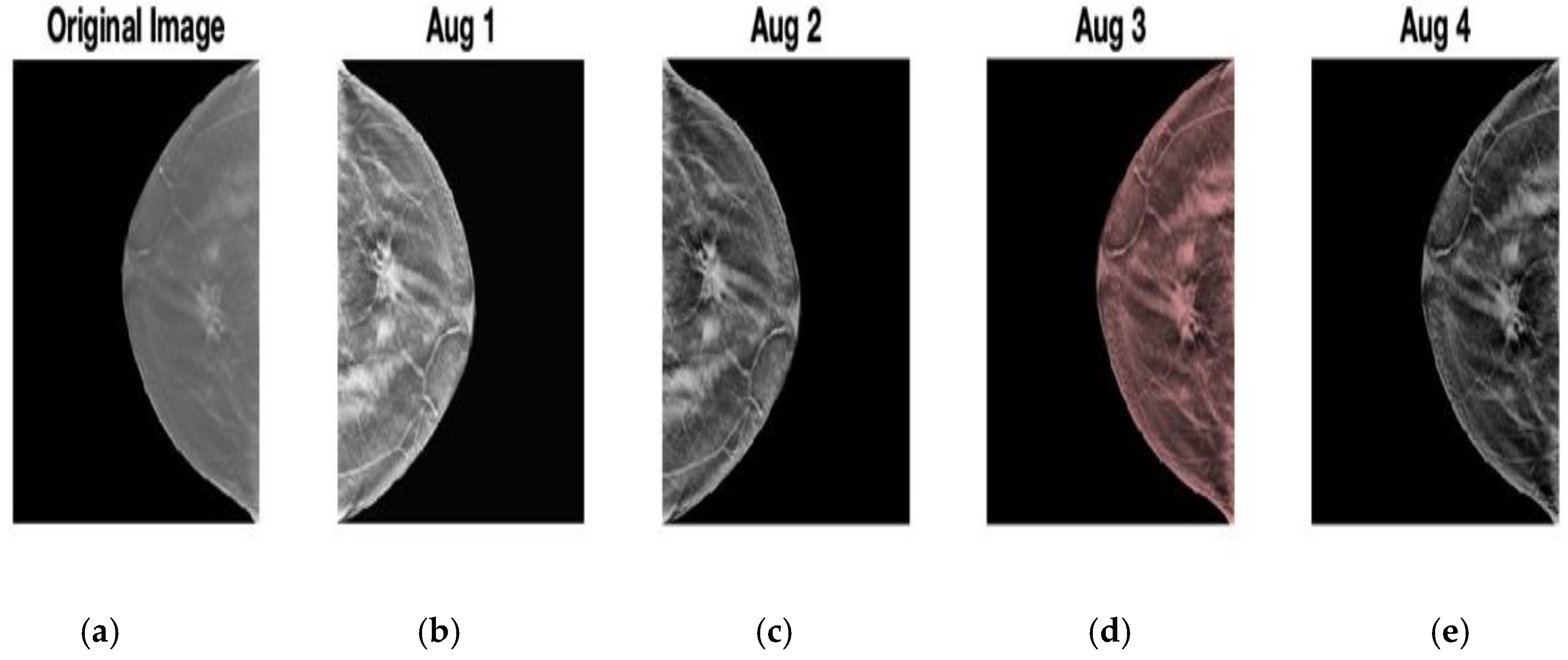
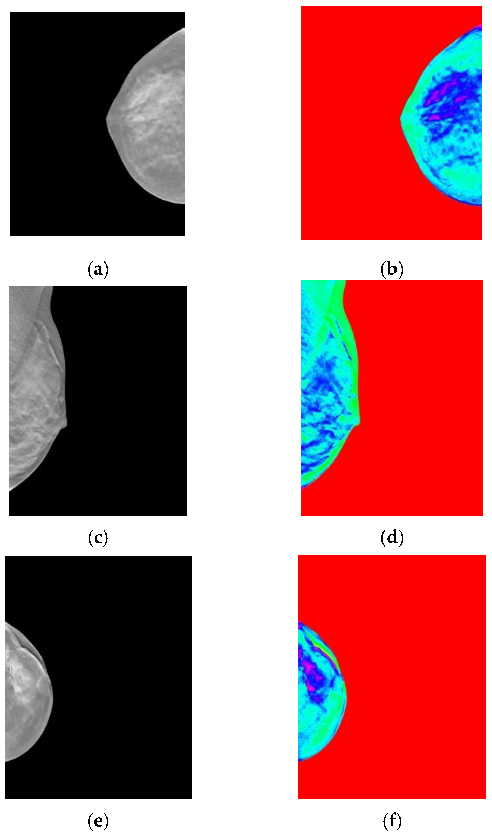
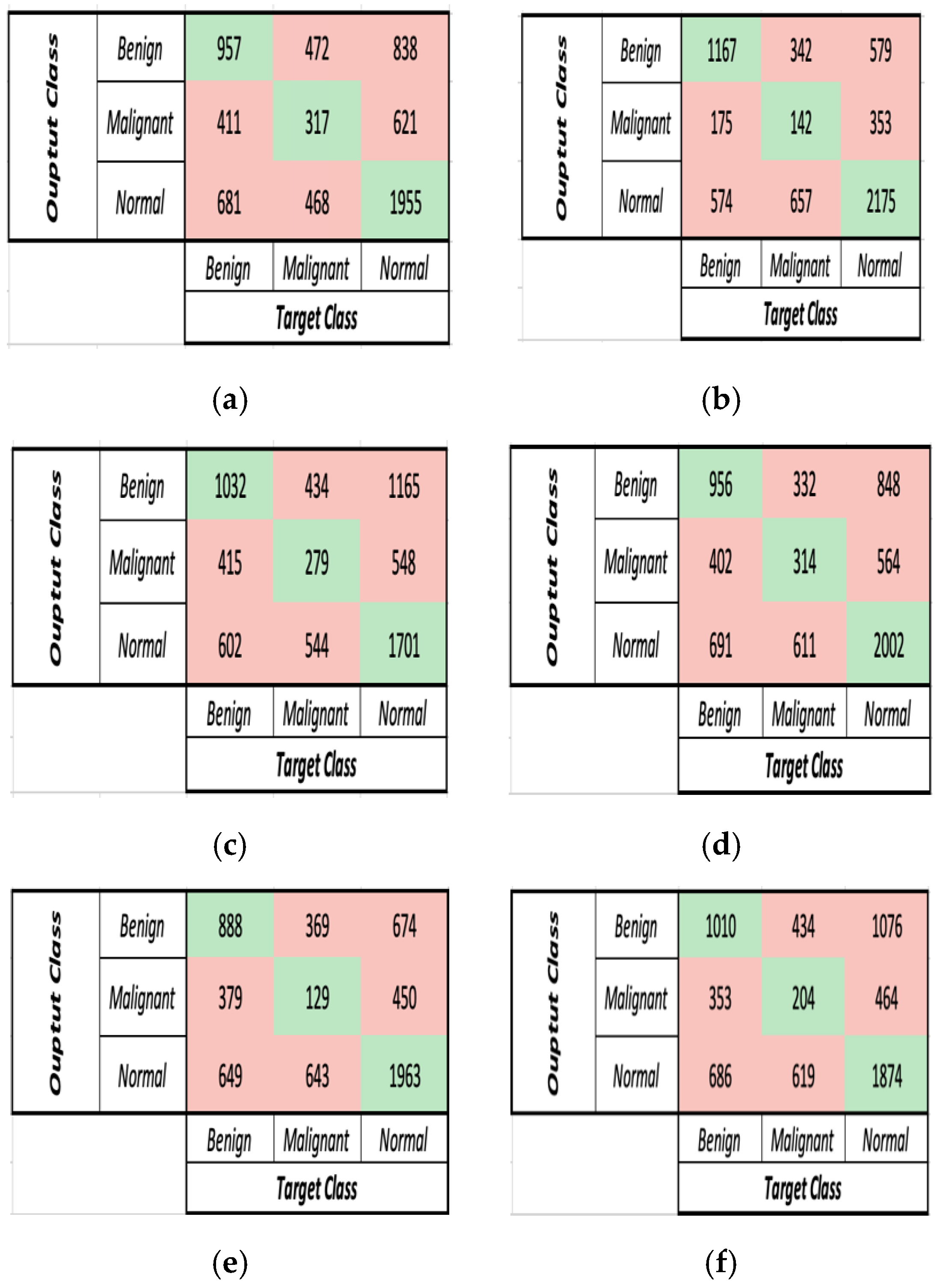
The performance of six deep learning models was compared twice for Dataset 1. In the first trial, after the augmentation stage, the images were passed to the colour feature map layer without using the image enhancement techniques mentioned in the pre-processing stage. In the second trial, DBT slices were augmented, then enhanced and a colour feature map was applied before being passed to the DL models. This was performed to check whether the image enhancement techniques proposed in the pre-processing stages improved the DBT classification performance or otherwise.

Figure 5 demonstrates the confusion matrices of the six deep learning models before applying the image and contrast enhancement techniques. The comparison between the DL models in terms of accuracy and run-time before pre-processing stage is presented in

Table 4. Comparison between the six DL models on Dataset 1 before pre-processing.

Deep Learning Model	Accuracy	Run-Time (s)
ResNet-18	48.05%	737
AlexNet	56.52%	706
GoogleNet	44.82%	916
VGG-16	48.69%	4301
MobileNetV2	48.67%	842
DenseNet-201	45.95%	4123

.

Table 4 and Figure 5 demonstrate that AlexNet obtained the highest accuracy and runtime, with an accuracy of 56.52% and a runtime of 706 s. With runtimes of 737, 4301, and 842 s, ResNet-18, VGG-16, and MobileNetV2 achieved accuracies of 48.05%, 48.69%, and 48.67%, respectively. Finally, GoogleNet and DenseNet-201 yielded the lowest accuracies of 44.82% and 45.95%, respectively, with runtimes of 916 and 4123 s.

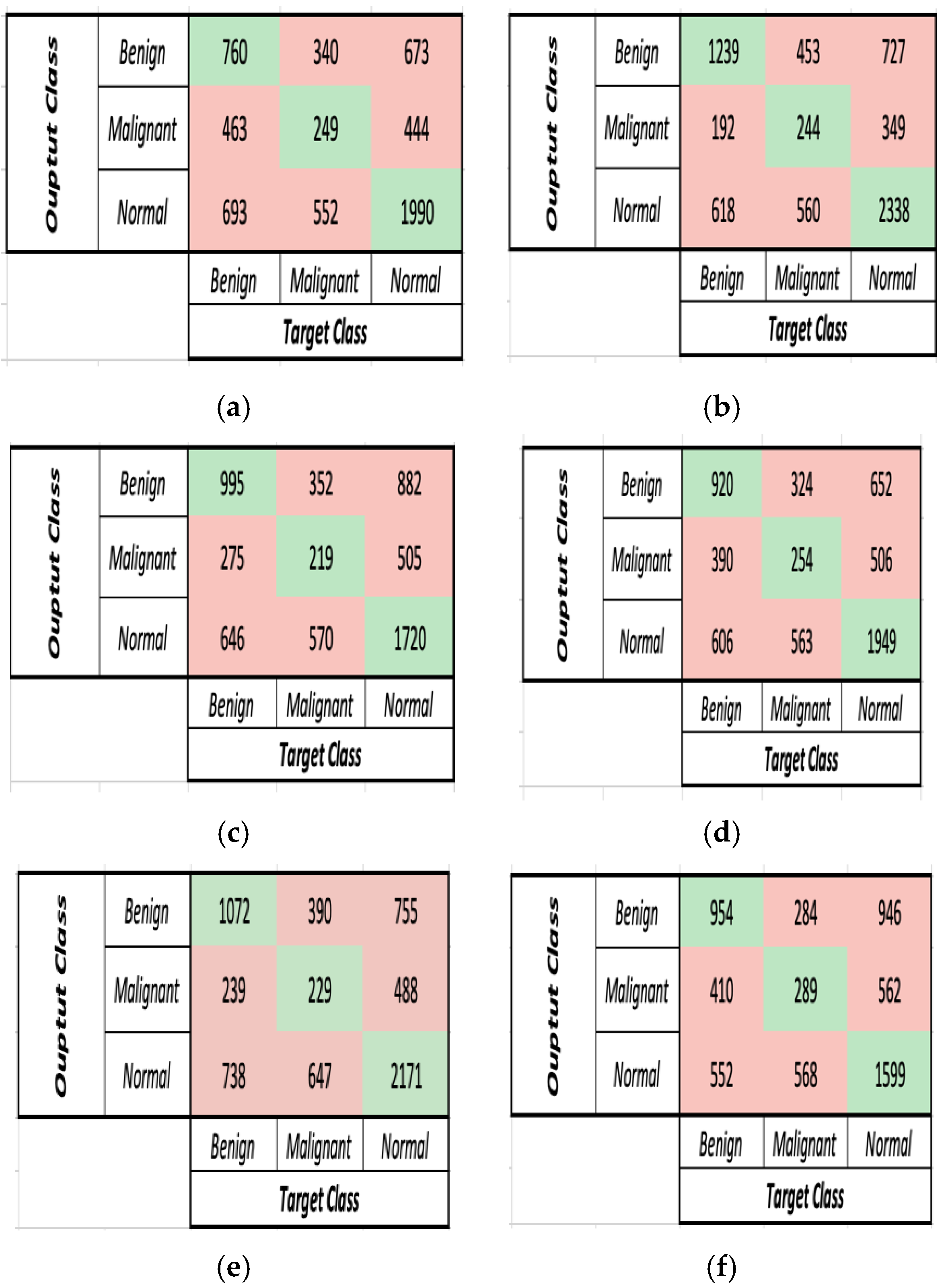
Figure 6 features the confusion matrices of the six deep learning models after implementing the pre-processing phase before the feature extraction phase. The comparison between the DL models in terms of accuracy and run-time after pre-processing is presented in Table S5.

Based on Table 4 and Table S5, it is concluded that the accuracy has improved in all DL models after applying the pre-processing stage. As for the run-time, AlexNet, ResNet-18, and MobileNetV2 needed less time to extract features from the enhanced images, thus reducing the run-time. Despite the insignificant increase in the run-time for GoogleNet, DenseNet-201, and VGG-16 there was an obvious increase in the accuracy of classification.

In terms of accuracy, after applying the image enhancement techniques, MobileNetV2 and GoogleNet managed to achieve the highest improvement of 2.86% and 2.78%, respectively. ResNet-18 and GoogleNet achieved an 0.6% and 2.78% accuracy improvement. Finally, AlexNet and DenseNet-201 recorded an improvement of 0.34% and 0.16%, respectively. In terms of runtime, ResNet-18, AlexNet and MobileNetV2 reduced their runtime by 11.9%, 7.68% and 7.36%, respectively. GoogleNet, VGG-16 and DenseNet-201, on the other hand, recorded an increase in their runtime by 24.5%, 10.6% and 8.63%, respectively.

B.

Dataset 2

More scans from patients with no findings (normal) were added to analyse the performance of the proposed model when adding more data for training and testing. Moreover, the performance of the deep learning models on Dataset 1 and Dataset 2 was compared in terms of accuracy and run-time after adding the pre-processing stage for both datasets. Dataset 2 featured multiple scans for patients from the following classes:

10.

Normal: 199 patients

11.

Benign: 62 patients

12.

Malignant: 39 patients

The comparison between the performance of the DL models on Dataset 2 in terms of accuracy and run-time (s) is documented in Table S6 and Figure 7a,b.

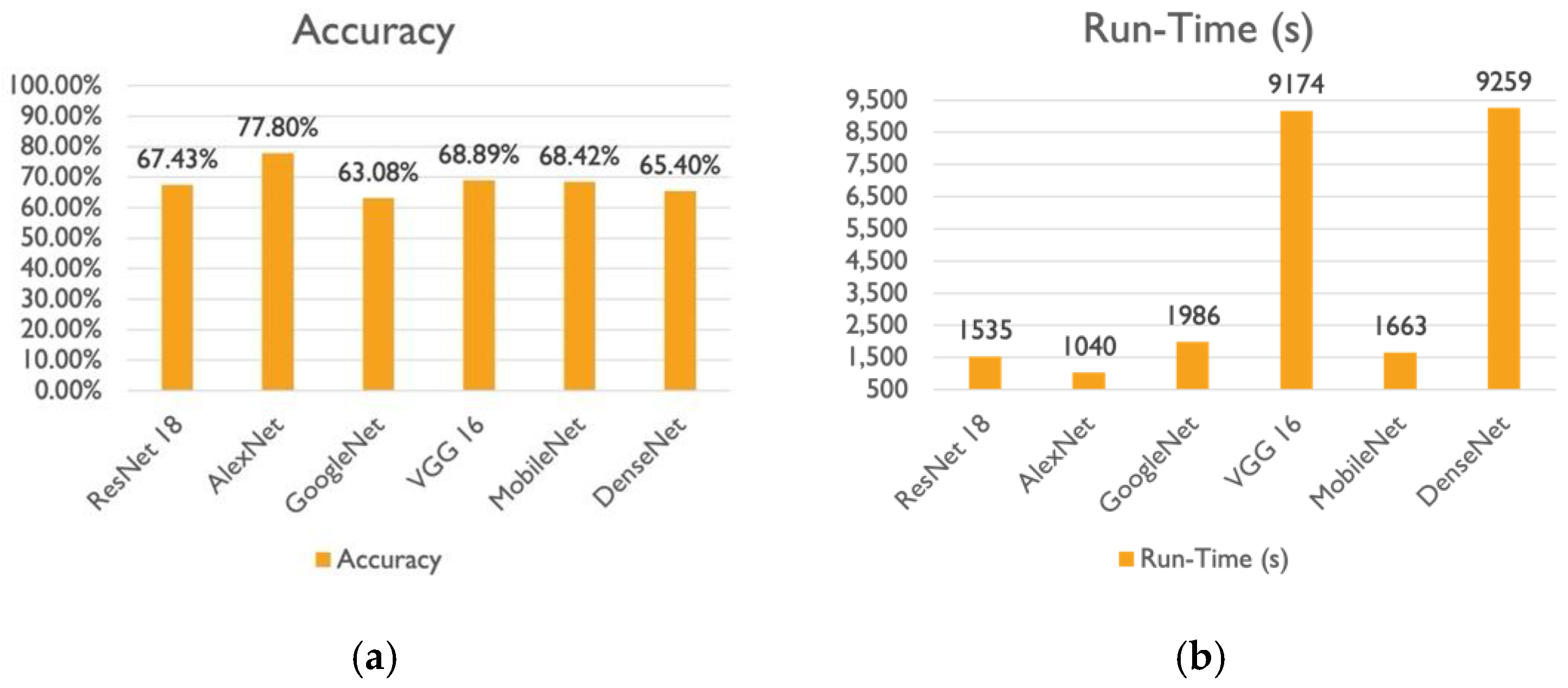
The comparison between the performance of the DL models on Dataset 2 in terms of accuracy and run-time (s) is documented in Table S6 and Figure 7a,b. Based on Table S6 and Figure 7a,b, it is proven that extracting features using AlexNet resulted in the best accuracy, and performance and less time was needed for training and testing, with an accuracy of 77.8% and runtime of 1040 s. Although MobileNetV2 and VGG-16 concluded with the approximately same accuracy, there is a noticeable difference in the computation time. VGG-16 took almost five times as long as MobileNetV2 to extract features. Following the three previously mentioned models, DenseNet-201 recorded the least accuracy of 65.40%, despite taking six times longer to extract features than ResNet-18. ResNet-18 achieved an accuracy of 67.43% with a runtime of 1535 s. Finally, in comparison to AlexNet, which performed the best, GoogleNet experienced a 14% drop in the model’s accuracy and a runtime of 1986 s.

A comparison between the performance of the DL models using Dataset 1 and Dataset 2 is provided in Table S7. Based on Table S7 using Dataset 2, AlexNet provided the best accuracy and run-time results, with a 21% gain in accuracy and the least percentage increase in runtime. On the other hand, the worst percentage increase in run-time was recorded with a 19% improvement in accuracy for ResNet-18. Moreover, VGG-16 and DenseNet-201 recorded the same percentage increase in run-time along with an accuracy increase of 18.22% and 19.29%, respectively. Finally, the least accuracy gain was observed when GoogleNet and MobileNetV2 were implemented to extract features, which increased the classification accuracy by 15.48% and 16.89%, respectively.

C.

Dataset 3

Finally, Dataset 3 was generated by adding extra data for training and testing, as well as new scans from patients who had no findings (normal) to analyse performance and compare it to Dataset 2 and Dataset 1 outcomes. Dataset 3 featured multiple scans for patients from the following classes:

13.

Normal: 499 patients

14.

Benign: 62 patients

15.

Malignant: 39 patients

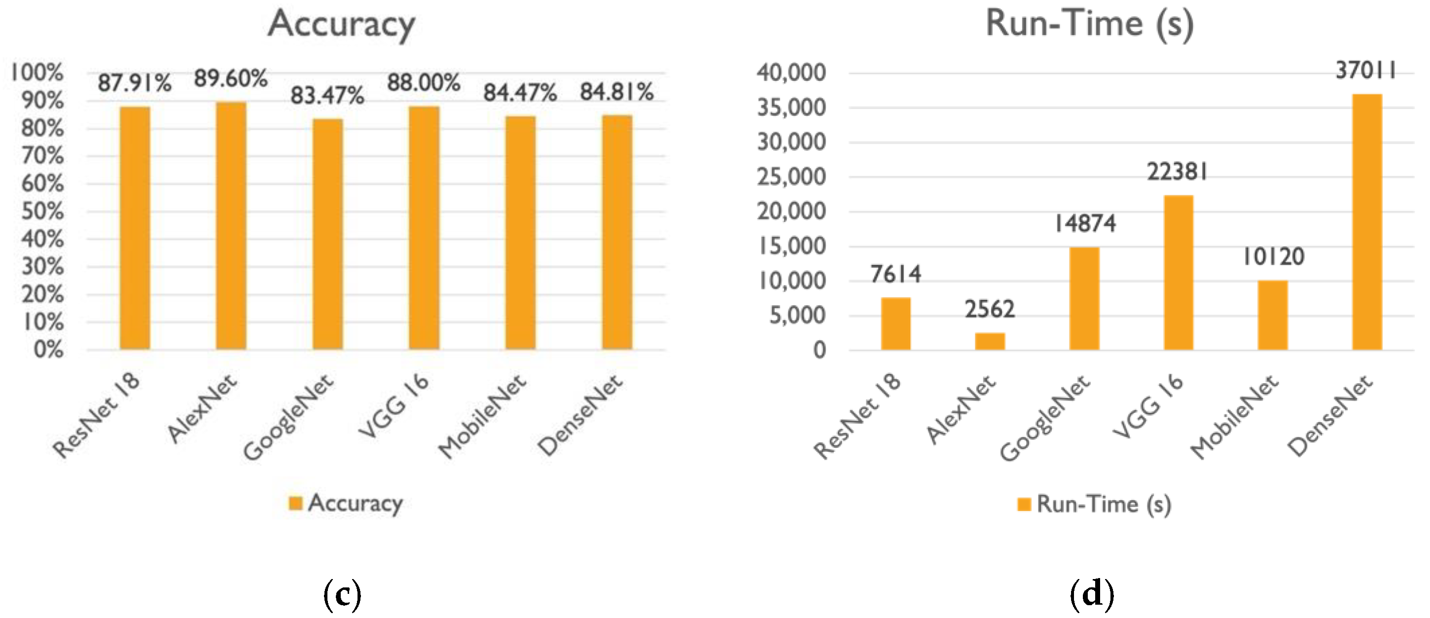
Table S8 and Figure 7c,d compare the accuracy and run-time (s) of the DL models on Dataset 3, respectively. According to Table S8 and Figure 7c,d, AlexNet recorded the highest classification accuracy of 89.6%, while GoogleNet recorded the lowest classification accuracy of 83.47%, and VGG-16 and ResNet-18 both achieved an 88% classification accuracy, but VGG-16 took nearly three times as long as ResNet-18 to achieve it. Finally, DenseNet-201 achieved the same accuracy as MobileNetV2 at 85%, but it took three times as long.

A comparison between the performance of the DL models using Dataset 2 and Dataset 3 is provided in Table S8. Table S8 demonstrated that Dataset 3 resulted in higher classification accuracy in all six DL models. VGG-16 and AlexNet exhibited the lowest increase in elapsed time, with accuracy gains of 19% and 12%, respectively. Additionally, Table S8 indicates that GoogleNet and ResNet-18 recorded the maximum improvement in accuracy, with a 20% increase. When compared to ResNet-18, GoogleNet experienced a considerable increase in computation time.

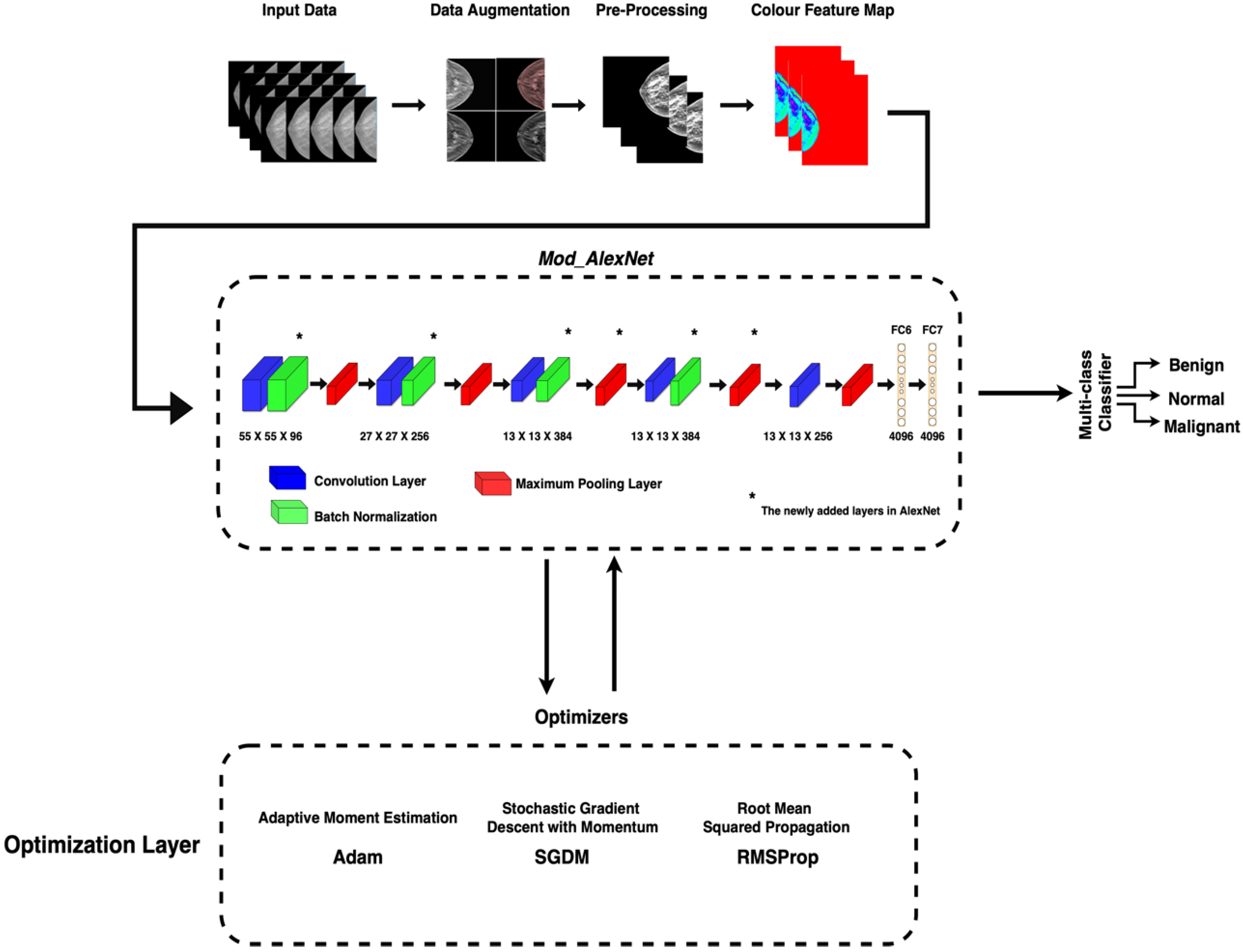
3.2. Second Scenario

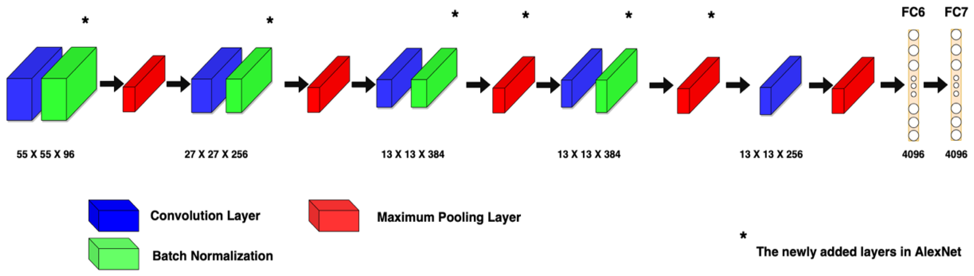
The first scenario concluded that AlexNet outperformed the other five DL models in DBT classification. As a result, a modified architecture (Mod_AlexNet) was developed to improve AlexNet’s performance.

The performance and accuracy of AlexNet and Mod_AlexNet were measured and compared using the metrics of accuracy, and loss. Due to the large size of the dataset, each training was performed for three epochs with batch sizes of 32, 64, and 512. The models were trained using a variety of optimisers, including adaptive moment estimation (Adam), root mean squared propagation (RMSProp), and stochastic gradient descent with momentum (SGDM).

A comparison between the performance of Mod_AlexNet and AlexNet in terms of training accuracy, training loss, and testing accuracy using different optimizers is shown in the following sections. The analysis was carried out on the 600 patients mentioned in Dataset 3.

• SGDM Optimizer

The comparison between the performance of Mod_AlexNet and AlexNet in terms of training accuracy, training loss, and testing accuracy using SGDM optimizer with different batch sizes is shown in

Table 5. SGDM optimizer performance (3 epochs and batch sizes: 32, 64, and 512).

DL Models	Batch Size	Training Accuracy	Testing Accuracy	Training Loss
AlexNet	32	98.50%	88.74%	0.05
	64	97.94%	88.53%	0.07
	512	93.33%	90.32%	0.2
Mod_AlexNet	32	97.67%	91.61%	0.08
	64	96.74%	90.63%	0.11
	512	91%	90.70%	0.26

and Figure S1.

Based on Figure S1, it is concluded that for a batch size of 32, AlexNet achieved a training accuracy of 98.50% and a training loss value of 0.05, while Mod_AlexNet achieved a lower training accuracy of 97.67% and a training loss value of 0.08 for the same batch size. Moreover, AlexNet achieved 97.94% training accuracy with a training loss value of 0.07, while Mod_AlexNet achieved 96.74% training accuracy with a training loss value of 0.11 for a batch size of 64. Finally, for a batch size of 512, AlexNet obtained 93.33% training accuracy with a training loss value of 0.2, while Mod_AlexNet achieved 91% training accuracy with a training loss value of 0.26.

Table 5 demonstrated that using the SGDM optimization technique, Mod_AlexNet outperformed AlexNet in terms of testing accuracy on different batch sizes. Mod_AlexNet recorded a 2.87% testing accuracy increase when compared to AlexNet with a batch size of 32. When training the models on 64 and 512 batch sizes, Mod_AlexNet exhibited a 2.1% and 0.38% increase in test accuracy when compared to AlexNet, respectively. The highest test accuracy was achieved on a batch size of 32 by Mod_AlexNet, with an accuracy of 91.61%.

B.

Adam Optimizer

The comparison between the performance of Mod_AlexNet and AlexNet in terms of training accuracy, training loss, and testing accuracy using Adam optimizer with different batch sizes is shown in

Table 6. Adam optimizer performance (3 epochs and batch sizes: 32, 64, and 512).

DL Models	Batch Size	Training Accuracy	Testing Accuracy	Training Loss
AlexNet	32	89.52%	88.67%	0.4
	64	89.50%	89.02%	0.4
	512	86.70%	89.26%	0.48
Mod_AlexNet	32	89.94%	90.26%	0.39
	64	94.01%	89.45%	0.18
	512	90.09%	90.36%	0.28

and Figure S2.

According to Figure S2, for a batch size of 32, Mod_AlexNet achieved a training accuracy of 89.94% and a training loss value of 0.39, whereas AlexNet achieved a lower training accuracy of 89.52% and a training loss value of 0.4. Furthermore, Mod_AlexNet achieved 94.01% training accuracy with a training loss value of 0.18 for a batch size of 64, whereas AlexNet achieved 89.50% training accuracy with a training loss value of 0.4. Finally, with a batch size of 512, Mod_AlexNet achieved 90.09% training accuracy with a training loss of 0.28, while AlexNet achieved 86.70% training accuracy with a training loss of 0.48.

Based on Table 6, Mod_AlexNet outperformed AlexNet in terms of testing accuracy on different batch sizes, according to the Adam optimization technique. When compared to AlexNet with a batch size of 32, Mod_AlexNet improved testing accuracy by 1.59%. Mod_AlexNet demonstrated a 0.43% and 1.1% increase in test accuracy when trained on 64 and 512 batch sizes, respectively, when compared to AlexNet. The highest test accuracy of 90.36% was achieved by Mod_AlexNet on a batch size of 512.

C.

RMSProp Optimizer

The comparison between the performance of Mod_AlexNet and AlexNet in terms of training accuracy, training loss, and testing accuracy using RMSProp optimizer with different batch sizes is shown in

Table 7. RMSProp optimizer performance (3 epochs and batch sizes: 32, 64, and 512).

DL Models	Batch Size	Training Accuracy	Testing Accuracy	Training Loss
AlexNet	32	87.21%	86.26%	0.72
	64	87.20%	89.13%	0.69
	512	86.69%	90.26%	0.50
Mod_AlexNet	32	93.18%	87.28%	0.25
	64	93.49%	90.32%	0.25
	512	84.17%	90.60%	0.52

and Figure S3.

Based on Figure S3, Mod_AlexNet outperformed AlexNet for a batch size of 32, with training accuracies of 93.18% and 87.21%, and training loss values of 0.25 and 0.72, respectively. Furthermore, for a batch size of 64, Mod_AlexNet achieved 93.49% training accuracy with a training loss value of 0.25, whereas AlexNet achieved 87.20% training accuracy with a training loss value of 0.69. Finally, with a batch size of 512, AlexNet achieved a higher training accuracy of 86.69% and a training loss of 0.50, while Mod_AlexNet achieved a lower training accuracy of 84.17% and a training loss of 0.52.

Table 7 demonstrates that according to the RMSProp optimization technique, Mod_AlexNet outperformed AlexNet in terms of testing accuracy on different batch sizes. Mod_AlexNet improved testing accuracy by 1.02% when compared to AlexNet with a batch size of 32. When trained on 64 and 512 batch sizes, Mod_AlexNet demonstrated a 1.19% and 0.34% increase in test accuracy, respectively, when compared to AlexNet. Mod_AlexNet achieved the highest test accuracy of 90.60% on a batch size of 512.

4. Discussion

DBT is a three-dimensional imaging modality that can reduce false negatives and false positives in tumour detection caused by overlapping breast tissue in traditional two-dimensional (2D) mammography. Clinical studies suggest CAD models can enhance the identification of breast cancer and aid radiologists in the decision-making process, increasing diagnostic accuracy. In this regard, a multi-class diagnosis system is proposed where a modified deep learning architecture is integrated with data augmentation and colour mapping techniques.

In this study, scans from the BCS-DBT dataset were augmented with different augmentation techniques to enhance the performance of the DL models by creating newly formed examples for the training set. Moreover, the DBT slices were enhanced with contrast and edge enhancement techniques in the pre-processing stage. Following the pre-processing, a colour mapping technique was applied to remove background artefacts and properly segment the breasts from the background. The features are then extracted using six different CNN. Finally, for each CNN, SVM is deployed to classify the images into three categories: normal, benign, and malignant. The three datasets were derived from the BCS-DBT dataset, which comprises information on 5060 patients. As shown by the experiments, the three datasets included scans from 200, 300, and 600 patients, respectively.

As shown by the experiments, AlexNet outperformed the five DL on all three datasets in terms of accuracy and runtime and proved to be a high-performing DL model in this imaging modality.

Furthermore, in this study, a new deep learning model (Mod_AlexNet) was developed to improve the performance of AlexNet. The traditional AlexNet now has six more layers, four of which are batch normalisation layers and two of which are maximum pooling layers.

AlexNet and Mod_AlexNet were tested against the BCS-DBT dataset with 600 patients in this study. Transfer learning was used on AlexNet and Mod_AlexNet, and each model was trained using a different optimization technique, such as SGDM, Adam, and RMSProp, each with batch sizes of 32, 64, and 512.

Moreover, different performance indicators were measured when comparing the performance of traditional AlexNet and the modified AlexNet (Mod_AlexNet) on Dataset 3 using different optimization techniques and batch sizes. AlexNet’s and Mod_AlexNet’s performance and accuracy were measured and compared using the metrics of training accuracy, testing accuracy, and training loss. Mod_AlexNet architecture outperformed traditional AlexNet in terms of test accuracy with improvement rates of 3.23%, 1.79% and 1.34% when compared using SGDM, Adam, and RMSProp optimizers, respectively. Mod_AlexNet achieved the highest test accuracy of 91.61% with a training accuracy of 97.67%, and a training loss value of 0.08 optimized by SGDM with a batch size of 32.

5. Conclusions

This paper introduces a new computer-aided multi-class diagnosis system with a modified deep learning architecture (Mod_AlexNet) that effectively classifies DBT scans. The proposed model incorporates augmentation and colour map segmentation techniques with a modified deep learning framework (Mod_AlexNet) for efficient diagnosis. An optimization layer with multiple high performing optimizers is appended to the proposed modified deep learning architecture (Mod_AlexNet) so that it can be evaluated and optimised using various optimization techniques. Investigations were carried out on a large breast tomography benchmark dataset. The proposed multi-class diagnosis system demonstrates the importance of incorporating DBT augmentation and colour feature map segmentation with an optimized deep learning architecture in terms of enhancing performance indicators. To efficiently classify DBT slices, two experimental scenarios are deployed. The first scenario proposed a computer-aided multi-class diagnosis (CAD) model that integrated DBT augmentation, image enhancement techniques, and colour feature mapping with six deep learning models for feature extraction. The second scenario used several optimization techniques with different batch sizes to compare the performance of the newly proposed Mod_AlexNet architecture and traditional AlexNet, and different evaluation performance metrics were computed. In the first scenario, AlexNet improved by 1.69%, 5.13%, 6.13%, 4.79%, and 1.6% when compared to ResNet-18, MobileNetV2, GoogleNet, DenseNet-201, and VGG16, respectively. While for the second scenario, when compared using the SGDM, Adam, and RMSProp optimizers, the proposed Mod_AlexNet architecture outperformed AlexNet in terms of test accuracy with an average improvement rate of 3.23%, 1.79% and 1.34%, respectively. Furthermore, because no underlying specific assertions were made that would inhibit generalisation, the proposed multi-class CAD system is a general framework that can be trained and applied to similar problems and imaging modalities. In the future, the proposed deep learning architecture (Mod_AlexNet) will be modified, and data from more patients will be used to support and enhance the deep learning model’s prediction.