Exploring the Nonlinear Effects of Built Environment on Bus-Transfer Ridership: Take Shanghai as an Example

Abstract

In this paper, the nonlinear effects of the built environment on bus–metro-transfer ridership are explored, based on Shanghai metro data, with an extreme gradient-boosting decision-trees (XGBoost) model. It was found that the bus-network density had the largest influence on transfer ridership, contributing 27.56% predictive power for transfer ridership, followed by closeness centrality and bus-stop density, and their contribution rates are 21.6% and 17.27%, respectively. Local explanations for the model reveal the following conclusions: most built-environment variables have nonlinear and threshold effects on bus–metro ridership. The suggested values for the dominant contributors to bus–metro-transfer ridership are obtained. For example, bus-network density, bus-stop density, and closeness centrality were 12.8 km/sq. km, 11 counts/sq. km, and 0.18 km/sq. km, respectively, for maximizing bus–metro-transfer ridership. The interaction impacts of the bus–metro connection characteristics and the closeness centrality of metro stations on transfer ridership were, also, examined. The result showed that the setting of bus–metro-transfer facilities depended on the location of metro stations. It was necessary to improve the bus–metro-connection system, in metro stations with high closeness centrality.

1. Introduction

Compared with the bus-travel mode mode, due to the more punctual and efficient characteristics, the metro-travel mode has, gradually, become the main commuting mode for passengers, such as in Singapore [1], Beijing [2], and Hong Kong [3]. In 2021, Singapore railways (including MRT lines and LRT lines) accounted for 42.8% of passenger volume (source: lta.gov.sg, accessed on 12 April 2022). Beijing rail transit accounted for 55% of passenger volume in 2021, in terms of a report on 24 May 2022 by the Beijing Daily. Hong Kong railways (including MTR Lines, the Airport Express Line, the Light Rail, and HK Tramways) accounted for only 40.1% of passenger volume in 2020, slightly lower than 2019, due to COVID-2019, according to the Statistical Department of Hong Kong Special Administrative Region. However, in suburban areas with underdeveloped transportation infrastructure, the metro system is unlikely to reach such a far place. Unlikely, since realizing door-to-door flexible service is one of the main disadvantages of the metro system. Thus, the feeder bus plays an important role in the collection and distribution of metro ridership. Under these circumstances, developing bus–metro-transfer hubs is the key measure to increasing transfer ridership and mitigating the traffic congestion prevalent in big cities today.

The development of buses and the metro was interdependent [4]. The rapid development of feeder buses gave full play to the potential positive impact of the metro system and expanded the radiation area of the metro system. Similarly, the development of the metro integrates the public transport network system resources along the metro lines to form a high-quality bus–metro-transfer system. Many previous studies are focused on the bus–metro-transfer hubs [5,6].

Previous empirical studies indicated that the built environment had a significant impact on bus–metro-transfer ridership [7]. The interaction between the built environment and bus–metro-transfer behavior did not always lead to maximum the attraction of metro. To foster metro ridership around stations, it was important to identify the relationship between the built environment and bus–metro-transfer ridership. Empirical studies on this topic, however, were limited [7].

Many studies using traditional regression models have been devoted to investigating linear associations between the built environment and transit ridership [8,9]. However, most of them were likely to ignore the pervasive nonlinear and moderating effects among built-environment variables.

The influence of the station-area built environment on metro-passenger generation may be influenced by the location and accessibility of stations [10]. For stations with different network attributes, understanding nonlinearity and moderating utility can help designers formulate targeted built-environment strategies. However, only a limited number of studies constructed the impact of network attributes on bus–metro ridership for metro stations [11]. Many other important factors should, also, be incorporated, when conducting the association analysis between bus–metro-transfer ridership and the built environment. In this paper, composed of multiple indicators, we establish a comprehensive index system to analyze the bus–metro-transfer behavior, including bus–metro connection characteristics, land-use attributes for trip attraction and production, network attributes of metro stations, and demographic factors.

By comparing with the traditional linear-regression model, random forest, and Light Gradient-Boosting Machine (LightGBM), the extreme gradient-boosting decision-trees (XGBoost) model is chosen to, quantitatively, reveal the nonlinear impact of the built environment on bus–metro ridership. XGBoost is a state-of-the-art machine-learning method, which can, conveniently, reveal the nonlinear or threshold effects of influential factors on bus–metro ridership. Moreover, the study applied a partial dependence plot to explain the marginal effect of built environment variables on the prediction results of the machine-learning model.

The contributions of this study, mainly, include: (1) quantifying the nonlinear effect of the built environment on bus–metro-transfer ridership in the most effective ranges and thresholds; (2) comparing the relative importance of different built-environment variables; and (3) analyzing the moderating impact of metro-station location on the relationship between the built environment and bus–metro-transfer ridership.

The remainder of this paper is organized as follows. Section 2, briefly, presents some of the literature on the association between the built environment and bus–metro-transfer behavior. Section 3 introduces the data sources and variables of this study. Section 4 describes the XGBoost model and features. Section 5 analyzes the results, to understand how the bus–metro connection characteristics, network attributes of metro stations, demographic factors, and land-use attributes affect the bus–metro-transfer ridership. Section 6 illustrates the research results, limitations, and future research directions.

2. Literature Review

Many previous studies on the functionality of public transport systems were, mainly, based on the passengers’ subjective feelings and the services provided by transport facilities. For instance, a study [11] found that the station-area built environment had a significant influence on transport interchanges in the UK and Finland. Another paper [12] studied the travel-mode selection of the Nanjing metro station, by using the hybrid logit model. Their research results showed that the bus–metro-transfer was one of the important travel modes. Research [13] established a large-scale complex hypernetwork, to find out the interconnection mechanism among the bus network, metro network, and bus–metro network. On the other hand, passengers’ transfer intention largely depended on their transfer feeling [14]. The study [15] applied structural equation modeling, to explore the impact of perceived values, free bus transfer, and penalties on passengers’ bus–metro-transfer intention. They found that the three factors all affect transfer intention between bus and metro.

In recent years, metro-smart-card data was commonly used for the research of passenger-travel behavior [16]. Metro-smart-card data have been collected to mine the data chain, such as origin–destination (OD) estimation [16], transit performance evaluation [17,18], and travel behavior analysis [19,20]. Based on the survey data from the metro smart card, many appropriate mathematical models have been established, to investigate the transfer behavior between bus and metro. For example, a study [21] developed a fast data-fusion method, based on combined data from bus smart cards and the GPS system, to explore station- and time-specific elapsed-time thresholds, according to the smart card data of Shenzhen, China. Another paper [22] provided a method to measure the transfer quality of bus–metro from two dimensions of time and space, using smart-card data and geographic-information-system (GIS) tools. Research [23] explored the transfer time of different intermodal connections and assessed the transfer service of intermodal connections, based on smart-card data. However, the correlation between the urban built environment and transfer ridership was not fully explored. The reasons may be that in their studies, the built environment was not explicitly described by special variables, such as the bus–metro connection characteristics, land-use attributes, and network attributes of metro stations.

The correlation between the built environment and transfer ridership can be investigated by linear and nonlinear models. The linear model may cause wrong analysis results, if built-environment variables have a threshold or nonlinear effect on ridership [24]. To solve this problem, some researchers used log-linear or the Poisson family, to eliminate the error caused by linear analysis [10,25,26]. Compared with nonlinear models, linear models addressed the theoretical significance of variables but ignored the practical significance and nonlinear influence of variables [27]. The nonlinear influence of variables was an urgent problem to be solved, in the field of urban-built-environment and travel behavior [28,29].

In previous studies, many built-environment variables were used for influence analysis on transfer behavior, such as the bus–metro connection characteristics [13], network attributes of metro stations [30], land-use attributes [31,32], and demographic factors [9]. For a better literature review of the previous related studies, we made a comparison table, shown in Table 1. Bus–metro connection characteristics have a long-term impact on transfer ridership. According to the relevant surveys, the transfer-connection characteristics among transportation modes had a significant impact on travelers’ choices, such as the distance, time, and connection characteristics of traffic transfer [22,30,33]. A paper [34] concluded that when rail transit did not connect with the bus, the travel preference of rail transit would be greatly reduced. The study [35] stated that the less transfer walking time and waiting time there is, the higher the probability of people choosing combination travel. According to a survey in Bangkok, Thailand, the transfer distance between metro stations and bus stations had a great impact on the travel satisfaction of the transfer behavior [36].

There was a close association between land-use attributes and bus–metro-transfer behaviors [37,38]. Research [39] compared the impact of land-use attributes for different networks and for individual travel modes. The results showed that integrated land use will actively encourage public transport travel. The study [40] explored the multimodal transport method in transportation planning. They found that reasonable planning of land use can bring huge benefits, especially a comprehensive land-use mode, composed of office, commerce, entertainment, and other work. There was a causal relationship between traffic and land use. The land-use attribute for trip production (residential density) plays an important role in promoting the growth of transfer ridership.

Table 1. Literature review of some previous studies, in terms of the four built-environment variables and methodology.

Citation	A			B		C						D			E	Methodology	Linear Model	Nonlinear Model
	A1	A2	A3	B1	B2	C1	C2	C3	C4	C5	C6	D1	D2	D3
[9]	✓				✓	✓	✓		✓		✓		✓		✓	Ordinary least squares	✓
[30]	✓			✓												Social network analysis	-	-
[31]		✓				✓	✓		✓		✓				✓	Geographically and temporally weighted regression	✓
[32]		✓				✓		✓	✓	✓	✓	✓			✓	Geographically weighted regression	✓
[36]			✓												✓	Ordinal regression models		✓
[38]	✓	✓			✓		✓			✓	✓	✓	✓		✓	Hybrid model	✓
[39]					✓	✓	✓			✓	✓		✓	✓		Multivariate linear model	✓
[41]			✓												✓	Fitting analysis		✓
[42]	✓	✓				✓			✓	✓						Multiple regression models	✓
[43]	✓	✓	✓												✓	Gravity-based regression model		✓
This paper	✓	✓	✓	✓	✓	✓	✓	✓	✓	✓	✓	✓	✓	✓	✓	XGBoost	-	✓

Notes: A represents the bus–metro connection characteristics; A1 represents the bus-network density; A2 represents the bus-stop density; A3 represents the average transfer distance. B represents the network attributes of metro stations; B1 represents the closeness centrality; B2 represents the distance to the central station. C represents the land-use attributes. C1 represents the commercial ratio; C2 represents the employment density; C3 represents the industrial ratio; C4 represents the residential ratio; C5 represents the land-use diversity; C6 represents the street density. D represents the demographic factors. D1 represents the age; D2 represents the population density; D3 represents the average house size. E represents the use of the smart card data.

Table 1. Literature review of some previous studies, in terms of the four built-environment variables and methodology.

Citation	A			B		C						D			E	Methodology	Linear Model	Nonlinear Model
	A1	A2	A3	B1	B2	C1	C2	C3	C4	C5	C6	D1	D2	D3
[9]	✓				✓	✓	✓		✓		✓		✓		✓	Ordinary least squares	✓
[30]	✓			✓												Social network analysis	-	-
[31]		✓				✓	✓		✓		✓				✓	Geographically and temporally weighted regression	✓
[32]		✓				✓		✓	✓	✓	✓	✓			✓	Geographically weighted regression	✓
[36]			✓												✓	Ordinal regression models		✓
[38]	✓	✓			✓		✓			✓	✓	✓	✓		✓	Hybrid model	✓
[39]					✓	✓	✓			✓	✓		✓	✓		Multivariate linear model	✓
[41]			✓												✓	Fitting analysis		✓
[42]	✓	✓				✓			✓	✓						Multiple regression models	✓
[43]	✓	✓	✓												✓	Gravity-based regression model		✓
This paper	✓	✓	✓	✓	✓	✓	✓	✓	✓	✓	✓	✓	✓	✓	✓	XGBoost	-	✓

Notes: A represents the bus–metro connection characteristics; A1 represents the bus-network density; A2 represents the bus-stop density; A3 represents the average transfer distance. B represents the network attributes of metro stations; B1 represents the closeness centrality; B2 represents the distance to the central station. C represents the land-use attributes. C1 represents the commercial ratio; C2 represents the employment density; C3 represents the industrial ratio; C4 represents the residential ratio; C5 represents the land-use diversity; C6 represents the street density. D represents the demographic factors. D1 represents the age; D2 represents the population density; D3 represents the average house size. E represents the use of the smart card data.

Previous studies showed that residential density was an important driving factor for passenger flow [44,45]. The paper [46] concluded that the ridership increased with the increase in residential density around the station area. The subsequent research showed that the land-use attribute for the trip attraction (employment density, land-use diversity, etc.) may be a more important factor for passenger flow [47,48]. The study [32] conducted an empirical study in Shenzhen, China. Their results suggested that employment density, mixed land use, and road density had significant impacts on the ridership of buses and the metro. However, the land-use attribute was not the only factor affecting the transfer ridership. The transfer ridership was, also, affected by some other factors, such as transfer tickets. When the price of transfer tickets was discounted, the transfer ridership will keep increasing [49]. Reasonably coordinating the relationship between land-use attributes and pricing policies could improve the proportion of intermodal travel [50,51,52].

The network attribute and location of transfer hubs have a certain impact on the ridership prediction. Closeness centrality was an important measure of station connectivity [53]. It was one of the important factors to predict the bus–metro-transfer ridership [54]. Research [30] found that closeness centrality was positively related to bus–metro-transfer ridership. On the other hand, previous research results on the impact of distance to CBD on metro ridership were inconsistent. A paper [55] found that the distance to CBD had no significant impact on the passenger flow. By contrast, some studies found that the ridership of metro stations in CBD was much higher than other stations, in Nanjing [9].

The demographic factors, also, affect transport-mode choices to serve distinct trip purposes [56]. Some previous studies examined the effects of demographic characteristics on passenger flow [25,57]. Demographic characteristics, such as age, per capita GDP, and car ownership were found to affect residents’ travel choices [26,48].

The influence of the built environment on transit ridership is not fully explored, although many studies are focused on this topic. For example, most previous studies, mainly, applied linear-regression models to examine the relationship between the built environment and transit ridership [8,9]. However, in the actual prediction process, if built-environment variables have nonlinear and threshold effects on transit ridership, the application of linear models will distort the research results [58].

Some previous studies confirmed that the built environment has a nonlinear impact on travel behavior [28,46,59]. Progress of machine-learning and interpretation methods can better help us understand the nonlinear and regulatory effect of the built environment on human travel behavior [24,27]. The advantage of the nonlinear model, highlighted by [60,61], showed that the methods can break through the limits of samples, to produce a more reliable and stable prediction. Besides, the methods can capture complicated correlations between independent variables and dependent variables because there are no limits on the pattern/shape of the relationship [62]. The nonlinear effects verified that the marginal influence of the built-environment variables on travel behavior depended on the value of the built-environment variables. The threshold effect was one of the nonlinear effects. When the marginal influence of built environment variables on travel behavior exceeded a certain threshold, the value of the dependent variable increased, decreased, or remain unchanged [63]. In recent years, scholars are more and more interested in the application of tree-based machine-learning methods (e.g., random forest, LightGBM, and XGBoost), to identify the nonlinear and moderating impact of the built environment on travel behaviors [7,45,46,64,65,66,67].

Compared with the linear model and other commonly used nonlinear models (e.g., random forest and LightGBM), XGBoost had a higher degree of fitting the data [68]. XGBoost was a scalable end-to-end tree-boosting system, which can provide the most accurate research results for many problems, and it solved real-world-scale problems with the least resources [69]. The XGBoost model had the advantage that the prediction results were more in line with the actual situation, and the results were easily explainable [41,70]. XGBoost, also, can further reveal the relative importance and practical significance of relevant independent variables.In this paper, based on the Shanghai metro-smart-card data, the XGBoost model was used to explore the influence of urban built-environment variables on transfer ridership. The following four aspects are examined: (1) Do the built-environment variables have nonlinear effects on bus–metro-transfer ridership? (2) Examining the relative importance of built-environment variables in predicting bus–metro-transfer ridership. (3) Identifying the threshold effects of built-environment variables to maximize bus–metro-transfer ridership. (4) Exploring the moderating impact of station location on the relationship between the built environment and bus–metro-transfer ridership.

3. Data and Variables

3.1. Study Area

With the rapid development of global megacities, sustainable development has, gradually, become a basic requirement of urban planning and governance [71]. The relevant research and discussions on urban optimization have attracted the attention of a great number of researchers [72,73,74,75]. Facing various traffic-congestion problems caused by urban expansion [76,77], the Shanghai government has taken actions to improve the coordinated transportation efficiency of bus–metro-transfer hubs, which is one of the key steps to accelerating the maturity of the public transport network covering the whole city. Based on some studies related to Shanghai metros, this paper selects the 88 metro stations located next to the metro lines, in Shanghai [78,79]. The metro-station areas selected in this study include both composite functional areas and single-residential functional areas.

The samples selected in this paper are only limited to the accessible walking range, of a one-kilometer radius, around the metro station. According to the master plan of Shanghai, a 15 min walking community has been established for residents, which can obtain the required public services through 15 min of walking. Therefore, the study takes the range of 15 min walking distance (1 km radius) from the metro station as the data-measurement range.

3.2. Data Sources

The data of this study came from the IC card data of bus–metro transfer, at 88 metro stations along 12 metro lines in Shanghai. According to the bus–metro-transfer data of the metro IC card of Shanghai Shentong Metro Group Co., Ltd. (Shanghai, China), on 1 September 2016, there were 685,351 preferential records of bus–metro transfer, at all stations of the Shanghai metro network. By filtering the station information, missing data and abnormal data were deleted. Finally, we obtained 275,919 valid pieces of data, from 88 metro stations in the study area.

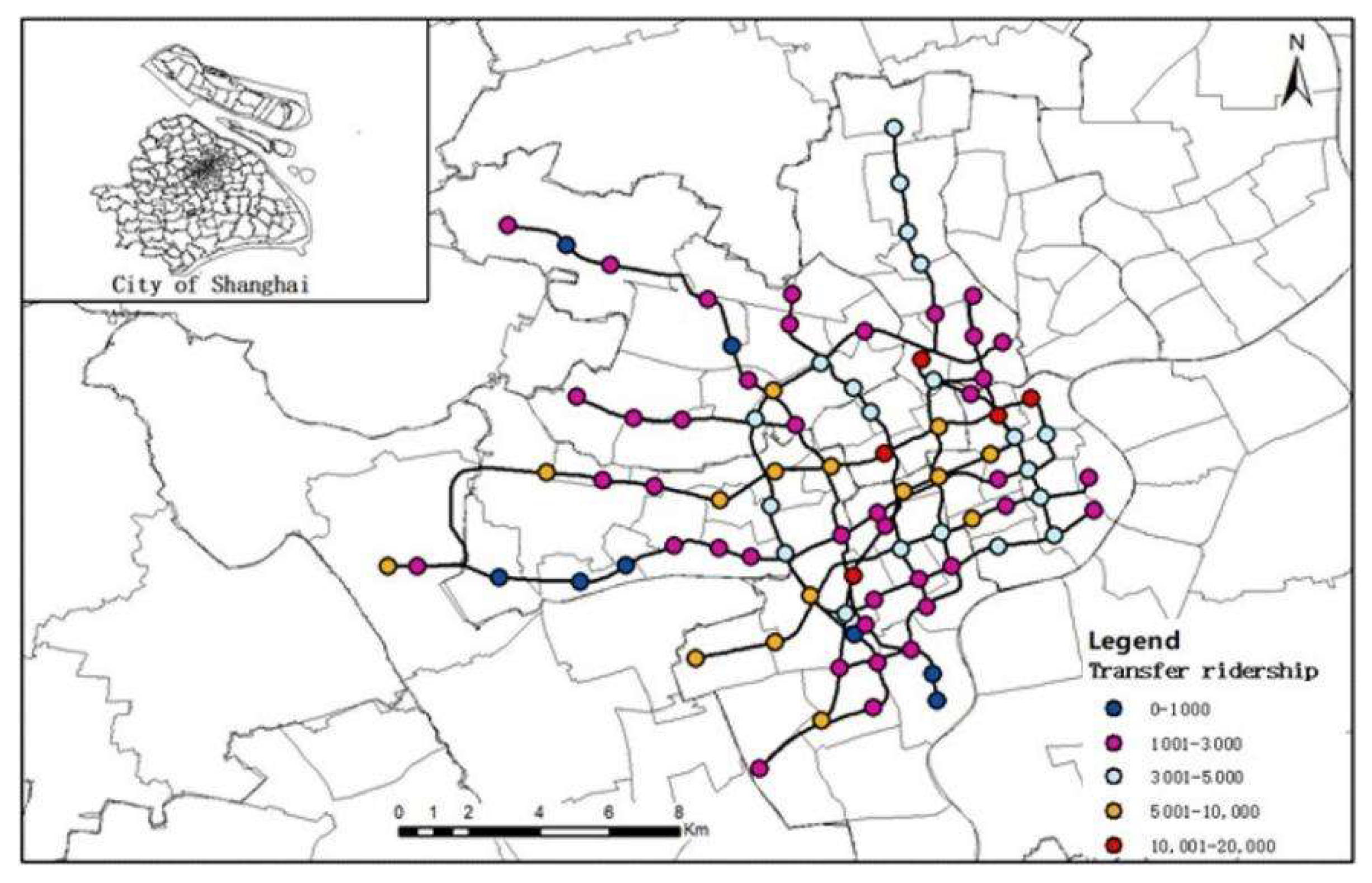
Figure 1 depicts the transfer ridership of bus–metro at 88 metro stations. Among them, the metro station with the largest transfer ridership is People’s Square, with 18,021 people, while Wuwei Road has the least transfer ridership, with only 366 people. There are 20 stations with more than 5000 people and 29 stations with less than 2000 people. The average daily transfer ridership is 3818 passengers per station.

Many studies showed that the relationship between the public transport system and rail transit system determined the population coverage of existing public services [80,81] and investment in transportation infrastructure [82,83]. Bus-network density has a greater impact on transfer ridership than other attributes of bus–metro connection characteristics.

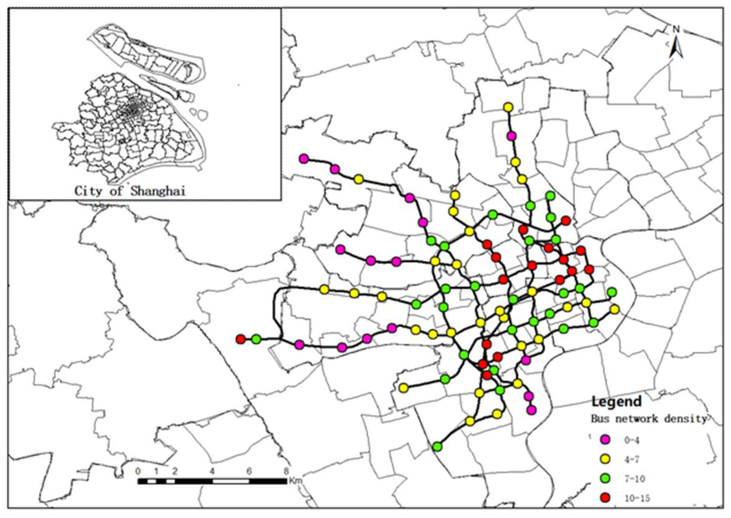
Figure 2 depicts the bus-network density within the 1 km radius of 88 metro stations. As shown in Figure 2, the average bus-network density is 7.46 km per square kilometer. Jing’an Temple station has the largest bus-network density, which is 14.97 km per square kilometer, indicating that the metro station has the fastest information transmission in the whole transportation network. The bus-network density around Hongqiao Airport Terminal 1 is the smallest, only 1.45 km per square kilometer, so the bus-network density needs to be further improved. During peak hours, in addition to connecting buses, passengers can, also, choose other potential services, to ensure the efficiency of existing transfer transportation services [84,85].

3.3. Variables Description

As shown in

Table 2. Variable description.

Variable Name	Description	Data Sources	Mean	S.D.	VIF
Dependent variable
Transfer ridership	Transfer ridership from bus to metro, of a metro station (thousand)	Metro smartcard data of Shanghai on 1 September 2016	3.82	3.17
Independent variables
Bus–metro connection characteristics
Bus-network density	The length of bus-network centerline per square kilometer (km/km2)	OpenStreetMap (OSM) data of 2020 Shanghai	7.46	3.29	3.46
Network repetition ratio of bus–metro	The repetition ratio R = L/S, where L is the parallel line of bus and metro, and S is the total bus line per square kilometer (km/km2)	OpenStreetMap (OSM) data, of 2020 Shanghai	0.13	0.05	1.32
Bus-stop density	Number of bus stops per square kilometer (counts/km2)	Point-of-interest (POI) data, of 2020 Shanghai	6.58	3.13	3.96
Average transfer distance	Average transfer distance, from bus stop to near metro (km)	Distance crawled from the Baidu Map (map.baidu.com, accessed on 12 April 2022)	0.2	0.05	1.40
Network attributes of metro stations
Distance to the central station	Network distance to Jing’an Temple station (km)	Distance crawled from the Baidu Map (map.baidu.com, accessed on 12 April 2022)	4.81	2.55	6.50
Closeness centrality	The closeness contrary, $\mathrm{C}=\frac{1}{{{\displaystyle \sum }}_{v-1}^{n-1}d\left(u,v\right)},$ where n is the number of all nodes in network, $d\left(u,v\right)$ is the shortest distance between node v and node u.	Distance crawled from the Baidu Map (map.baidu.com, accessed on 12 April 2022)	0.15	0.02	4.40
Land-use attributes for trip attraction
Employment density	Number of jobs per square kilometer (thousand/km2)	Point-of-interest (POI) data, of 2020 Shanghai	33.34	16.68	2.17
Industrial ratio	The ratio I = areas, for industrial use/all land areas	Land-use data, of 2020 Shanghai	0.05	0.11	2.69
Commercial ratio	The ratio C = areas, for commercial use/all land areas	Land-use data, of 2020 Shanghai	0.16	0.11	2.01
Land-use attributes for trip production
Residential ratio	The ratio R = areas, for residential use/all land areas	Land-use data, of 2020 Shanghai	0.38	0.14	2.78
Other land-use attributes
Land-use diversity	Entropy index of land use (0–1): $\frac{-{{\displaystyle \sum }}_{i=1}^m\left(s_i\right)ln\left(s_i\right)}{ln\left(m\right)},$ Where m is the type of land use, $s_i$ is the ratio of type-I land use to the total land area.	Land-use data, of Shanghai 2020	0.61	0.1	2.43
Street density	Length of the road/area size (km/km2)	OpenStreetMap (OSM) data, of 2020 Shanghai	7.67	3.00	2.57
Demographic factors
Car ownership	Ratio of workers with private cars, in average housing scale	Shanghai Statistical Yearbook 2020	0.63	0.08	1.45
Population density (ages between 20 and 44)	Population between 20 and 44 years old per square kilometer (thousand person/km2)	Shanghai Statistical Yearbook 2020	0.41	0.04	1.47
Local population density	Local population per square kilometer (thousand person/km2)	Shanghai Statistical Yearbook 2020	32.5	24.98	4.56
Average age	Average age of the residential in the area	Shanghai Statistical Yearbook 2020	42.01	0.92	1.40
PGDP	Per capita gross domestic product (104 RMB per capita)	Shanghai Statistical Yearbook 2020	4.41	1.96	3.14
Housing price	Average house prices near metro station (103 RMB per square meter) 2021.6	Baidu 2020	91.14	17.7	3.00
Average house size	Average house scale per kilometer	Shanghai Statistical Yearbook 2020	2.53	0.09	1.38

, we determine the dependent variables and independent variables and select the daily transfer ridership of the bus–metro as the dependent variable. The four built-environment variables are considered, namely bus–metro connection characteristics, land-use attributes for trip attraction, land-use attributes for trip production, and network attributes of metro stations as well as demographic factors.

The network repetition ratio of bus–metro reflects the direct contradiction between the metro and general bus. The repetition ratio was calculated by the ratio of the parallel line of bus and metro to the total bus line, within the research scope [86]. It reflects the passenger-flow-competition relationship and the connection relationship between the bus and metro. The average network repetition ratio of bus–metro in this paper is 0.13, which shows that there is no inevitable competitive relationship between bus and metro in Shanghai.

4. Methodology

We select the XGBoost model to predict the transfer ridership at bus–metro-transfer stations and rank the relative importance of the independent variables. The nonlinear relationship between the bus–metro-transfer ridership and important independent variables as well as the threshold adjustment utility is explained by generating a partial dependence plot.

XGBoost was an extensible tree-enhancement system and a kind of boosting algorithm [69]. The core idea of boosting the algorithm was to add many base models together, to form a strong classifier. XGBoost combined many CART trees. When data cannot be well fit by one tree, multiple CART trees were used to approach it, instead [87]. The advantage of the XGBoost model is adding a regularization term and second-order Taylor expansion, to avoid over-fitting in the high-precision calculation.

The model prediction output of XGBoost is shown in Equation (1):

$$\widehat{y}={\displaystyle \sum }_{k=1}^K{f}_k\left(x_i\right)$$

(1)

where $\widehat{y}$ is the sum of the prediction results of k samples, $f_k\left(x_i\right)$ is the prediction result of the k-th sample.

The loss function is shown in Equation (2):

$$\mathcal{L}={\displaystyle \sum }_{i=1}^{N}l\left(y_i,{\widehat{y}}_i\right)+{\displaystyle \sum }_k\mathrm{\Omega }\left(k\right)$$

(2)

where $l$ is a common loss function used to measure the difference between the actual value of each sample $y_i$, and the predicted value of each sample $\widehat{y}$, $\mathrm{\Omega }\left(k\right)$ is a regularization term, which describes the complexity of the tree. The complexity of decision tree k can be defined as Equation (3):

$$\mathrm{\Omega }\left(k\right)=\gamma ·T+\frac{1}{2}\lambda {\displaystyle \sum }_{j=1}^T{\omega }_j^2$$

(3)

where T is the number of leaf nodes in the decision tree, ${\omega }_j$ is the score of each leaf, and $\gamma$ and $\lambda$ are penalty parameters. ${\mathcal{L}}^{\left(t\right)}$ is the t-th round objective function, obtained through continuous iterative optimization, which can be described as Equation (4):

$${\mathcal{L}}^{\left(t\right)}={\displaystyle \sum }_{i=1}^{n}l\left(y_i,{\widehat{y}}_i{}^{\left(t-1\right)}+q_t\left(x_i\right)\right)+\gamma ·T+\frac{1}{2}\lambda {\displaystyle \sum }_{j=1}^T{\omega }_j^2$$

(4)

where $q_t$ is the addition example of the t-th iteration, carry out the second-order Taylor expansion at ${\widehat{y}}_i{}^{\left(t-1\right)}$ to, continuously, approximate the value of the objective function, as shown in Equation (5):

$${\mathcal{L}}^{\left(t\right)}={\displaystyle \sum }_{i=1}^n\left[l\left(y_i,{\widehat{y}}_i{}^{\left(t-1\right)}+g_i{q}_t\left(x_i\right)+\frac{1}{2}{h}_i{q}_t^2\left(x_i\right)\right)\right]+\gamma ·T+\frac{1}{2}\lambda {\displaystyle \sum }_{j=1}^T{\omega }_j^2$$

(5)

where $g_i={\partial }_{{\widehat{y}}^{\left(t-1\right)}}l\left(y_i,{\widehat{y}}_i{}^{\left(t-1\right)}\right), h_i={\partial }_{{\widehat{y}}_i{}^{\left(t-1\right)}}^{2}l\left(y_i,{\widehat{y}}_i{}^{\left(t-1\right)}\right)$. Since we only need to consider the variables in optimization, the constant term is removed, and all samples will, eventually, fall on a leaf node, no matter which way they go. Therefore, the combined formula can be written as shown in Equation (6):

$${\widehat{\mathcal{L}}}^{\left(t\right)}={\displaystyle \sum }_{j=1}^T\left[\left({\displaystyle \sum }_{iϵI_j}{g}_i\right){\omega }_j+\frac{1}{2}\left({\displaystyle \sum }_{iϵI_j}{h}_i+\lambda \right){\omega }_j^2\right]+\gamma ·T$$

(6)

where $I_j=\left\{i|q\left(x_i\right)=j\right\}$, represents the sample set falling on the j-th leaf node.

The selection of features and the correlation between features and prediction targets largely determines the prediction accuracy of this study. Due to the complexity of influencing factors, such as bus–metro connection characteristics, land-use attributes, network attributes of metro stations, and demographic factors, with the existing single-machine-learning model, it is difficult to solve the problem of multicollinearity processing of multi-source data. The high correlation between features can, also, reduce the robustness of the model, resulting in over-fitting in training. It is necessary to reprocess the multi-source transfer data to obtain the features with strong correlation with the prediction target.

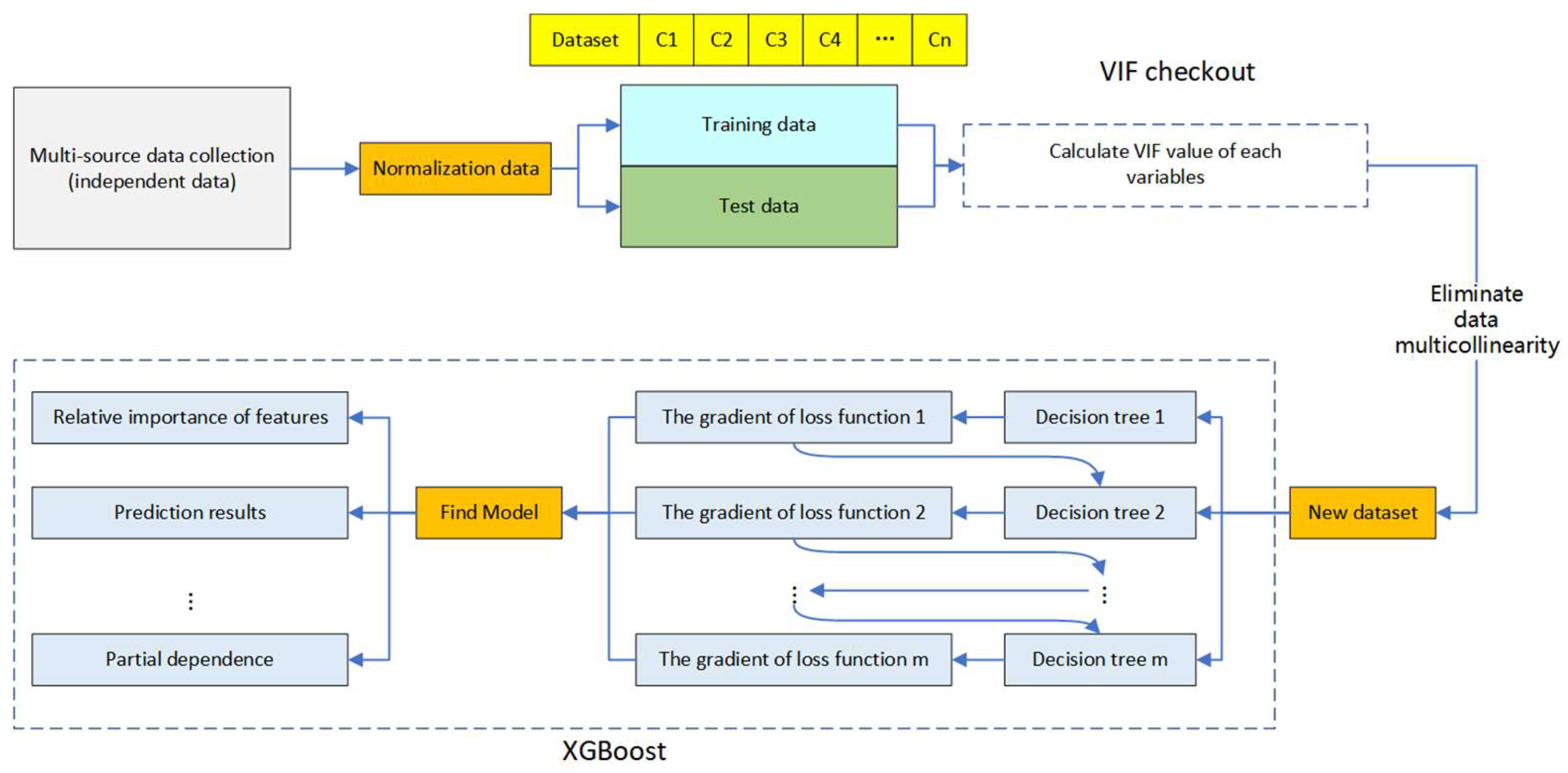
After solving the multicollinearity problem of multi-source data, the new dataset is substituted into the XGBoost model, for further prediction and analysis. The overall model framework of this paper is shown in Figure 3.

5. Results and Discussion

5.1. Model Comparison

Firstly, we eliminate the multicollinearity effect of data. We use the variance inflation factor (VIF) to judge whether there is multicollinearity between independent variables. The larger the VIF, the more serious the multicollinearity problem is. If the VIF exceeds 10, the multicollinearity of the data needs to be processed. As shown in Table 2, the average VIF value in this paper is 2.74, of which the maximum VIF value is 6.5, less than 10, so there is no need to worry about the multicollinearity between independent variables. The specific VIF test value is in Table 2.

To avoid over-fitting and reduce generalization error, we use a five-fold cross-validation procedure to train the model, in order to get the best parameter setting and result. In this paper, the parameters are listed as follows: the tree complexity is 10, the shrinkage parameter is 0.01, and the number of iterations and maximum trees is 10,000. After running the XGBoost model, we obtained the final results, with the minimum RMSE and R² of approximately 0.821.

To examine the advantage of XGBoost over traditional linear and nonlinear models, we conducted a comparison analysis between the traditional-linear model, random forest, LightGBM, and XGBoost, based on mean absolute error (MAE) and mean square error (MSE). The result shown in

Table 3. Comparison of the traditional linear and nonlinear model.

Metrics	Traditional Linear Model	Random Forest	Light GBM	XGBoost
R2	0.701	0.594	0.603	0.821
MAE	0.247	0.125	0.105	0.098
MSE	0.065	0.027	0.023	0.017

indicates that the R² of XGBoost model is 0.821, the mean absolute error (MAE) is 0.098, and the mean square error (MSE) is 0.017. The MAE and MSE of XGBoost are much smaller than other linear or nonlinear models, suggesting that XGBoost has a better fitting degree. The XGBoost model has the maximum R² value. Thus, this paper applies XGBoost to reveal the non-linear impact of built-environment variables on bus–metro-transfer ridership. The model can identify the rank of relative importance for the influential factors and improve the interpretability of the decision-making framework.

5.2. Relative Importance of the Independent Variables

Table 4. The relative importance of independent variables in predicting transfer ridership.

Variables	Relative Importance (%)	Rank
Bus–Metro Connection Characteristics (53.77%)
Bus-network density	27.56	1
Bus-stop density	17.27	3
Network repetition ratio of bus–metro	8.49	4
Average transfer distance	0.45	15
Network attributes of metro stations (22.1%)
Closeness centrality	21.6	2
Distance to the central station	0.5	14
Land-use attributes for trip attraction (5.39%)
Commercial ratio	3.28	7
Employment density	1.97	9
Industrial ratio	0.14	16
Land-use attributes for trip production (0.11%)
Residential ratio	0.11	17
Other land-use attributes (0.77%)
Land-use diversity	0.72	12
Street density	0.05	18
Demographic factors (17.86%)
Average age	6.18	5
Population density (age between 20 and 44)	5.73	6
Average house size	2.26	8
Car ownership	1.68	10
Local population density	1.37	11
PGDP	0.63	13
Housing price	0.01	19

illustrates the relative importance of independent variables and the rank of relative importance in the prediction process. The importance of all independent variables was measured by relative importance, and the sum of their total importance was 100% [88]. The main findings and relative contribution of all the independent variables on global scale are presented in a bulleted list.

• As shown in Table 4, the bus–metro connection characteristics account for 53.77%, and the bus-network density is the most significant factor affecting transfer ridership, accounting for 27.56%, which is consistent with the results of [89]. The relative contribution rates of bus-stop density, network repetition ratio of bus–metro, and average transfer distance are 17.27%, 8.49%, and 0.45%, respectively. Similar to [30], this result emphasizes the importance of forming interfaces between different transportation systems.
• The location of metro stations in a transit network plays an important role in predicting transfer ridership, accounting for 22.1%. Closeness centrality is an important index to measure the transfer efficiency of bus–metro, ranking second among all variables, and the relative contribution rate is 21.6%. The distance to the central station has a small correlation with transfer ridership, respectively.
• The land-use attributes for trip attraction play a great guiding role in increasing the attraction of rail transit [90]. In this paper, the land-use attributes for trip attraction account for 5.39%, especially the commercial ratio, which contributes 3.28%. By contrast, the land-use attributes for trip production only account for 11%, which influence the ridership slightly. The result shows that the developed business circle in a region will drive the development of the surrounding bus–metro combined travel.
• In terms of demographic factors, population density (ages between 20–44) is an important factor, with a contribution rate of 5.37%, which can be attributed to younger employees that prefer to travel by public transport. The regional PGDP reflects the private car ownership in the region, to a certain extent. The number of private cars has a negative impact on passengers’ bus-travel mode, so the number of private cars should be reduced [49,91,92].

5.3. Nonlinear Effect between Built Environment and Bus–Metro-Transfer Ridership

This section may be divided by subheadings. It should provide a concise and precise description of the experimental results, their interpretation, as well as the experimental conclusions that can be drawn.

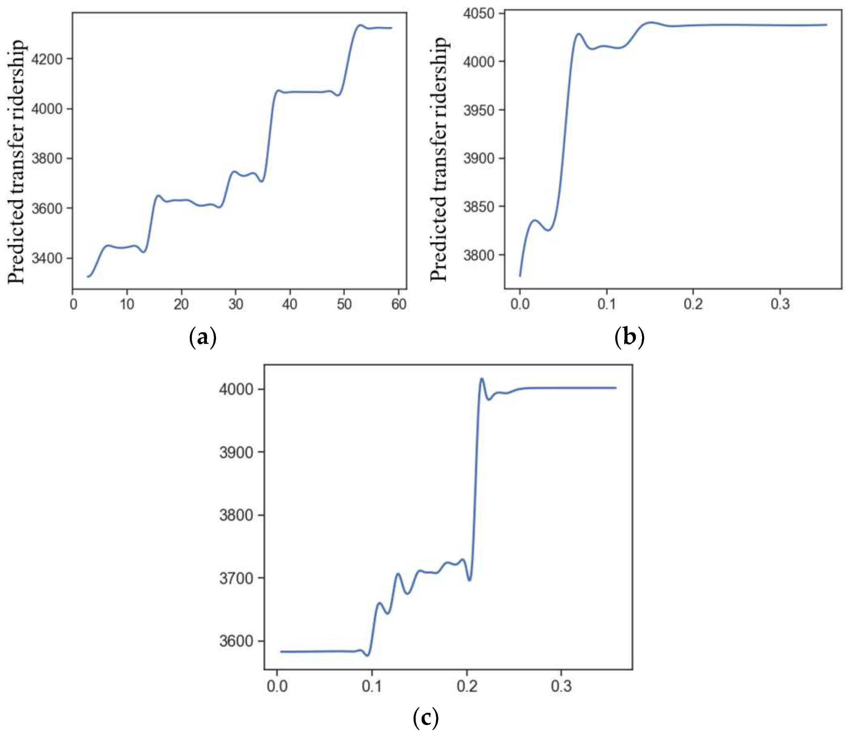
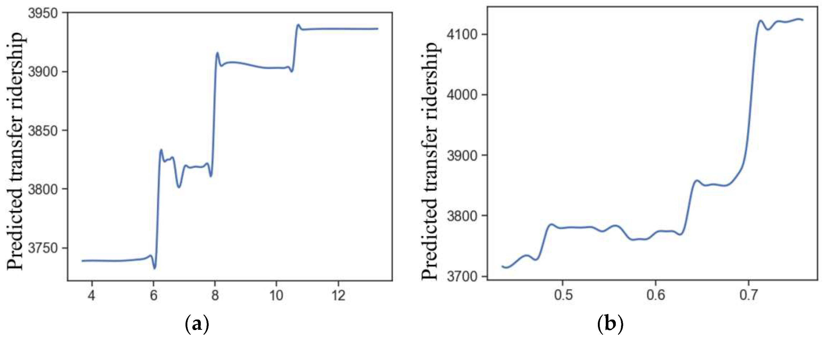
Figure 4 describes the nonlinear influence of the four independent variables of the bus–metro connection characteristics on transfer ridership. Figure 4a shows the positive association between bus-network density and bus–metro-transfer ridership. When the bus-network density around metro stations is 4 km to 11 km per square kilometer, the transfer ridership shows a slow upward trend. When the bus-network density is 11 km to 13 km per square kilometer, the transfer ridership increases rapidly. However, the transfer ridership decreases slightly between 11 km and 12.5 km. When it rises to about 7000, the transfer ridership tends to be stable, after a period of time. The result implies that increasing the bus-network density helps increase the transfer ridership. It, however, has little effect on attracting transfer ridership, when the bus-network density increases to a threshold of 12.8 km per square kilometer.

Figure 4b shows the significant nonlinear relationship between the average transfer distance and bus–metro-transfer ridership. Transfer ridership presents a higher value, when the average transfer distance is between 0.15 km and 0.18 km. This implies that the transfer distance within the range has a high attraction for travelers, to travel with the bus–metro combination. When the average transfer distance exceeds 0.18 km, the transfer distance has a negative impact on the transfer ridership, indicating that too large a transfer distance will reduce the transfer intention of passengers. Similarly, a study [35] explored that the less transfer walking time and waiting time there is, the higher the probability of people choosing combined travel. Research [92] obtained the conclusion that it was better to build new metro stations within 0.55 km, around existing bus stations, and within 0.25 km, of new bus stations, around the existing metro stations.

Figure 4c illustrates the positive influence of the network repetition ratio of bus–metro on the bus–metro-transfer ridership. When it is less than 0.07, the repetition ratio has almost no effect on transfer ridership. When the repetition ratio increases from 0.07 to 0.2, the transfer ridership increases continuously, but it decreases slightly between 0.11 and 0.115. When the repetition ratio exceeds 0.2, the transfer ridership tends to be stable. The result shows that the lower network-repetition ratio of bus–metro is not conducive to form a closely connected bus–metro-transfer hub. Within the closely connected range of the bus network and the metro network, the bus can transport people, in areas that cannot be radiated by railways, to metro stations.

Figure 4d displays the significant nonlinear association between bus-stop density and bus–metro-transfer ridership. When the bus-stop density is 2 counts to 7.5 counts per square kilometer, the bus-stop density has a positive influence on the transfer ridership. For each additional station within this interval, an average of 116 transfer passengers will be added. When the bus-stop density exceeds 5 per square kilometer, the transfer ridership keeps decreasing with the increase in bus-stop density. It has almost no effect on the bus–metro-transfer ridership, when the bus-stop density increases to 11 per square kilometer, and the transfer ridership will tend to be stable.

Figure 5 depicts the marginal impact of network attributes, based on metro stations on transfer ridership. Figure 5a suggests that closeness centrality has a positive influence on the bus–metro-transfer ridership. When closeness centrality is less than 0.15, there is almost no change in transfer ridership. By contrast, when closeness centrality increases from 0.15 to 0.18, transfer ridership increases, by about 5000 passengers. Once it is above 0.18, the corresponding transfer ridership slightly decreases. This result is reasonable. The stations of closeness centrality of more than 0.18 are central stations. These central stations are the travel destination of most passengers. In other words, only within a certain interval of closeness centrality does it have a significant impact on bus–metro-transfer ridership. In comparison with traditional studies on bus–metro-transfer ridership, this result is not fully explored.

Figure 5b demonstrates that the distance to the central station has a positive impact on transfer ridership. The farther away from the central station, the more bus–metro-transfer ridership there is. Due to the punctual characteristic and large capacity of the Shanghai Metro, many passengers work in the city center and live in the suburbs. During morning peak hours, passengers commute by the combined mode of bus and metro.

Figure 6 illustrates the nonlinear influence, of the four independent land-use attribute variables for trip attraction, on the transfer ridership. Figure 6a shows the threshold effect of employment density on transfer ridership. When the employment density is less than the threshold, it has a positive impact on transfer ridership, which is consistent with many previous studies [9,57]. When the employment density is above the threshold, increasing the number of jobs has almost no impact on transfer ridership. The result shows that a reasonable distribution of jobs around metro stations will improve the attractiveness of bus–metro transfer, but over-densification may lead to traffic chaos and overload, thus reducing people’s willingness to travel by public transport [29].

Figure 6b,c illustrate the nonlinear effects of the industrial ratio and the commercial ratio on the bus–metro-transfer ridership. As shown in Figure 6b, the industrial ratio has a positive impact on transfer ridership. When it grows from 0.05 to 0.09, transfer ridership increases by about 205 passengers, in an almost linear way. By contrast, when the industrial ratio is above 0.2, the change of industrial ratio has no effect on transfer ridership. However, the over-densification of industry will lead to traffic congestion, which will bring inconvenience for people to travel by public transport.

Figure 6c depicts the positive impact of commercial ratio on the bus–metro-transfer ridership. When the ratio is less than 0.1, it has a trivial effect on transfer ridership. When the commercial ratio increases from 0.1 to 0.22, transfer ridership keeps increasing. Transfer ridership remains stable, when the commercial ratio reaches the threshold. For urban planners, these trends can be considered to maximize bus–metro-transfer ridership.

Figure 7a,b show the nonlinear effects of street density and land-use diversity on bus–metro-transfer ridership. Figure 7a shows that the increase in street density has a positive impact on transfer ridership, when the street density is between 6 km and 11 km per square kilometer. Specifically, when the street density is between 6 km and 8 km per square kilometer, the climbing rate reaches the maximum. Similarly, other studies obtained the positive influence of the road density and public transport services on bus and metro [7,9,32].

Figure 7b shows that there is a significant nonlinear effect of land-use diversity on bus–metro-transfer ridership. When land-use diversity is above 0.7, transfer ridership increases rapidly to the peak. The trend becomes stable, when the threshold is reached.

5.4. Interaction Effects of Bus–Metro Connection Characteristics and Closeness Centrality on Transfer Ridership

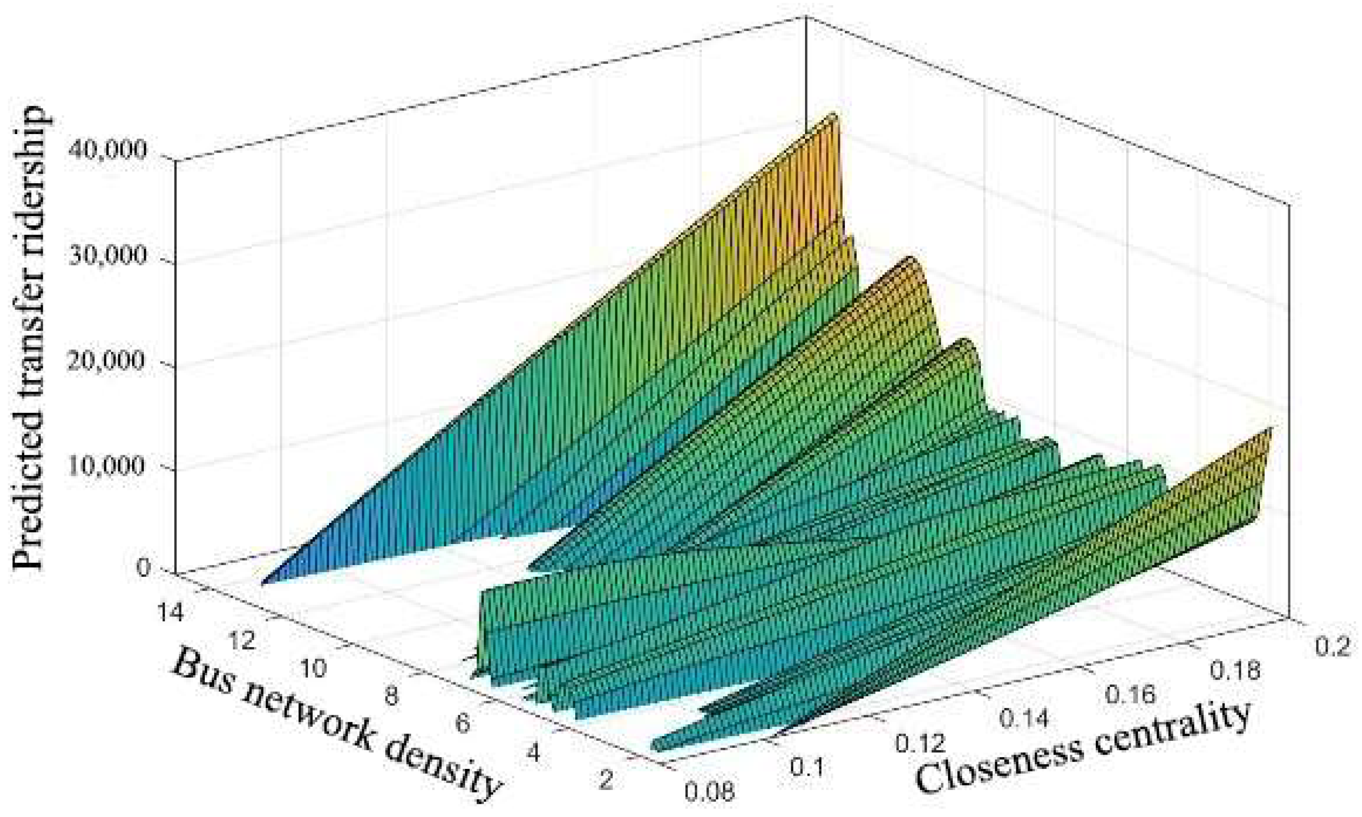
This study, further, investigates the interaction impact of bus–metro connection characteristics and closeness centrality on bus–metro-transfer ridership. Figure 8 demonstrates that the interaction influence of bus-network density and closeness centrality on transfer ridership is multivariate and nonlinear. As shown in Figure 8, when bus-network density ranges from 12 km to 14 km per square kilometer, and closeness centrality is more than 0.1, transfer ridership keeps sharply increasing. The transfer-ridership growth peaks at closeness centrality of 0.2 and bus-network density of 14 km per square kilometer.

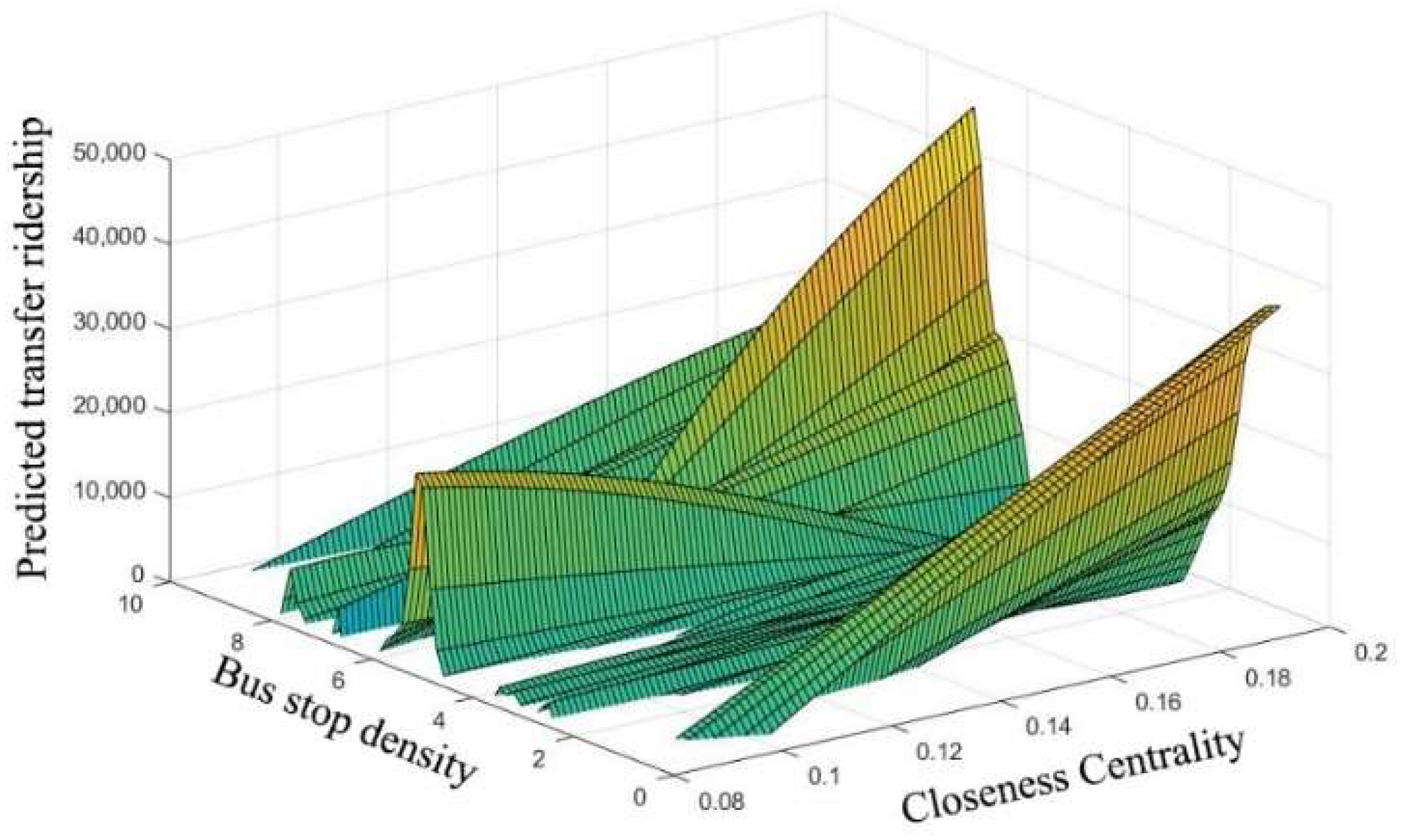
Figure 9 depicts the interaction effects of bus-stop density and closeness centrality on transfer ridership. The result indicates that when the density of bus stops is 6 to 8 per square kilometer, and closeness centrality is between 0.18 and 0.2, we can get the maximum transfer ridership. This finding can help planners to reasonably arrange the number of bus stops, according to the location attribute of metro stations.

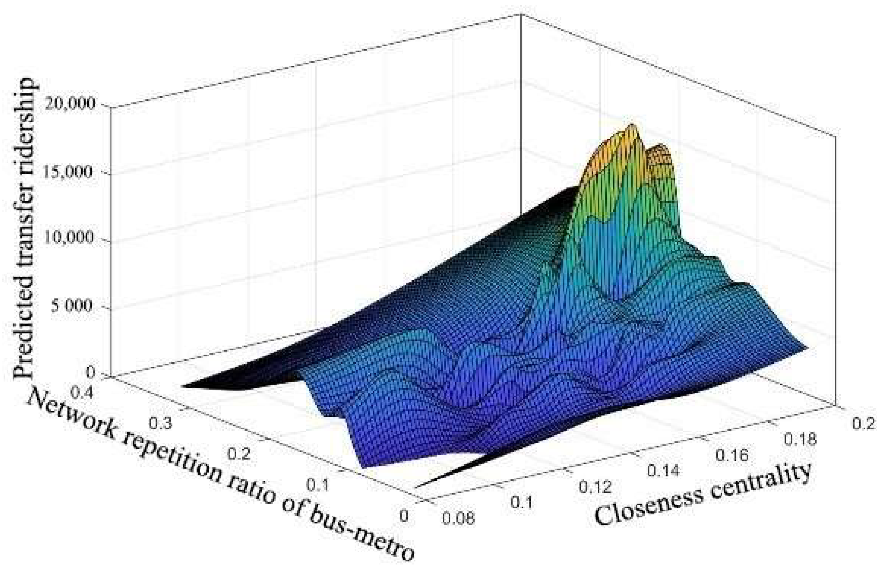
Figure 10 illustrates the combined effects of the network repetition ratio of bus–metro and closeness centrality on transfer ridership. We found that when the repetition ratio ranges from 0.2 to 0.3, closeness centrality is more than 0.16, and transfer ridership remains a high value, respectively. The finding can provide significant suggestions for the commercial planners of transportation network companies.

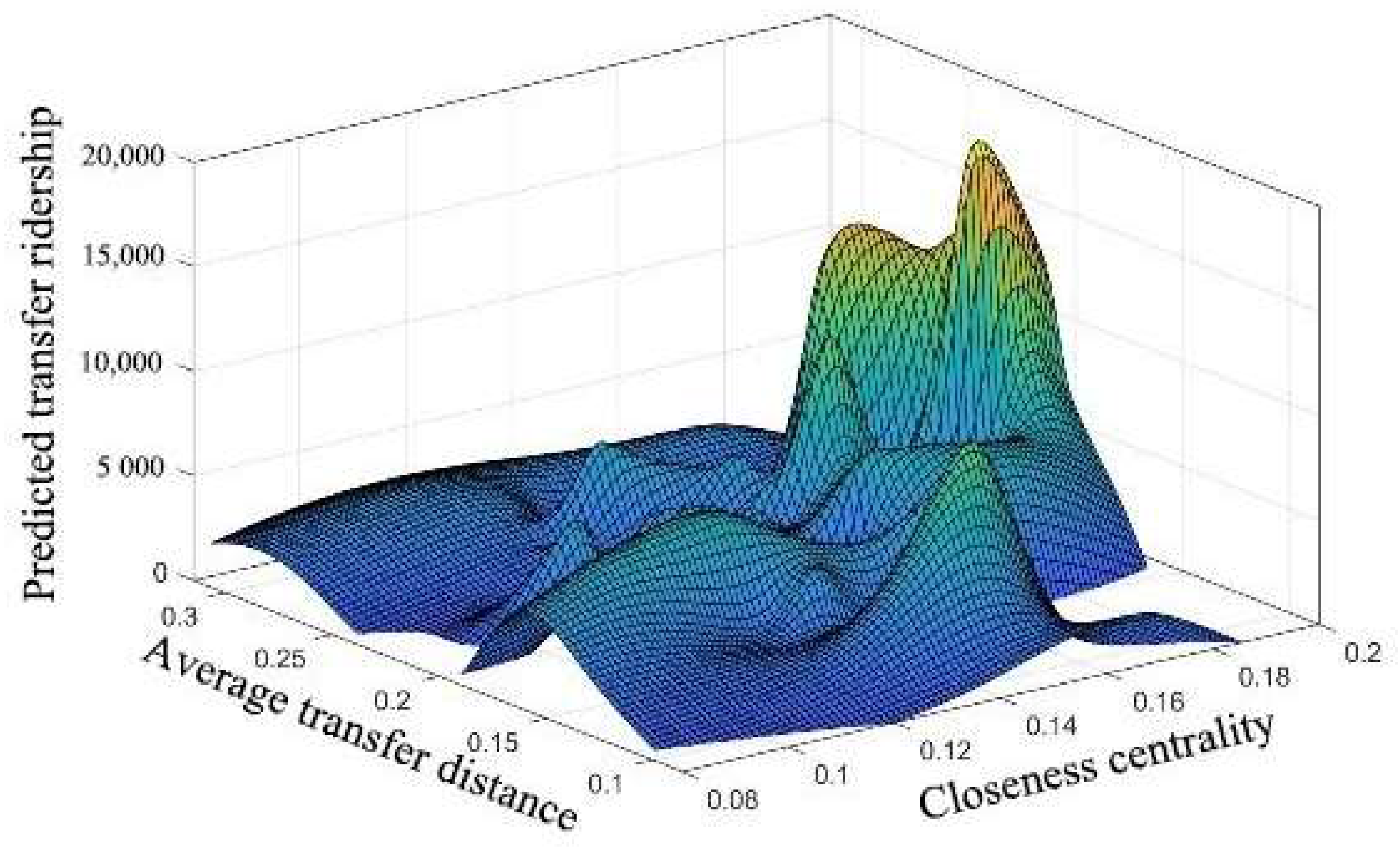
Figure 11 describes the influence of average transfer distance and closeness centrality on transfer ridership. The result shows that when the average transfer distance grows from 0.2 km to 0.25 km, and closeness centrality is more than 0.17, transfer ridership keeps stable growth. Transfer ridership reaches the peaks at the station, with a closeness centrality of 0.19.

The above results indicate that the setting of a bus–metro connection should be considered, together with the network attribute of the metro stations. This result implies that the bus–metro connection characteristics around stations depend on the stations’ positions.

6. Conclusions

This paper applied the XGBoost model to study the nonlinear impact of the Shanghai built environment on bus–metro-transfer ridership. The results put forward reasonable suggestions for urban architectural planning and TOD development.

Firstly, we carried out the correlation analysis of the independent variables and eliminated the adverse impact of the multicollinearity of the data on the model. Then, the new dataset was substituted into the XGBoost model, to obtain the relative importance rank of independent variables, for predicting transfer ridership. Finally, we analyzed the nonlinear effects of independent variables on transfer ridership.

The results indicate that the bus–metro connection characteristics (relative importance is 53.77%) have the largest impact on bus–metro-transfer ridership. The four key variables are bus-network density (relative importance is 27.56%), bus-stop density (relative importance is 17.27%), network repetition ratio of bus–metro (relative importance is 8.49%), and average transfer distance (relative importance is 0.45%).

These findings are useful for the bus–metro-transfer-facilities design of the metro-station areas. A station with higher closeness centrality can attract more transfer ridership. This means that the bus–metro-transfer facilities should be improved at the central stations. The land-use attributes for trip attraction have an important impact on bus–metro-transfer ridership. Among them, the commercial ratio has the most significant influence, with a relative importance of 3.28%, followed by the employment density, with a relative importance of 1.97, and the industrial ratio, with a relative importance of 0.14%. These findings are useful for TOD planners to establish land-use guidelines [7,44].

The research results of this paper can better help urban planners and transportation departments understand how the change of urban built environment affects the bus–metro-transfer ridership. The increase in the bus-network density, in areas without the provision of metro service, can provide travel convenience for residents. The employment density and commercial ratio have positive impact on the transfer ridership. To increase the mobility of the travel population and improve transfer ridership, the concentrated business circle around metro stations should be appropriately arranged.

Compared with the traditional models, the XGBoost model provides a more accurate and stable data-processing method. It can conduct integration analysis with various factors, in the presence of big data.

There are, however, some limitations in this study. For example, this paper only uses the one-day IC-card data of Shanghai’s 88 metros. In fact, it can further accurately conduct the impact of the built environment on bus–metro-transfer ridership, through the continuous time data of multiple cities. Most of the independent variables selected in this paper are exogenous factors, due to limited resources. The passengers’ travel attitude and travel preference are very important factors in the prediction process of transfer ridership. In the future, these endogenous factors can be taken into account.

References

- Adnan, M.; Biran, B.-H.N.; Baburajan, V.; Basak, K.; Ben-Akiva, M. Examining impacts of time-based pricing strategies in public transportation: A study of Singapore. Transp. Res. Part A Policy Pract. 2020, 140, 127–141. [Google Scholar] [CrossRef]
- Wang, M.; Mao, B.; Yang, Y.; Shi, R.; Huang, J. Determining the Level of Service Scale of Public Transport System considering the Distribution of Service Quality. J. Adv. Transp. 2022, 2022, 1–14. [Google Scholar] [CrossRef]
- Ding, L.; Zhang, K.; Xie, B. Incorporating Space-Time Correlation of Population Densities into the Design of a Candidate Rail Transit Line over Years. Discret. Dyn. Nat. Soc. 2021, 2021, 1–12. [Google Scholar] [CrossRef]
- Yue, M.; Kang, C.; Andris, C.; Qin, K.; Liu, Y.; Meng, Q. Understanding the interplay between bus, metro, and cab ridership dynamics in Shenzhen, China. Trans. GIS 2018, 22, 855–871. [Google Scholar] [CrossRef]
- Zhao, D.; Wang, W.; Li, C.; Ji, Y.; Hu, X.; Wang, W. Recognizing metro-bus transfers from smart card data. Transp. Plan. Technol. 2018, 42, 70–83. [Google Scholar] [CrossRef]
- Li, J.; Lu, Y.; Ling, L. The Integration of Public Bicycle and Metro Transit: A Case Study in Suzhou, China. In ICTE 2019; American Society of Civil Engineers: Reston, VA, USA, 2020. [Google Scholar] [CrossRef]
- Gan, Z.; Yang, M.; Feng, T.; Timmermans, H.J. Examining the relationship between built environment and metro ridership at station-to-station level. Transp. Res. Part D Transp. Environ. 2020, 82, 102332. [Google Scholar] [CrossRef]
- Loo, B.; Chen, C.; Chan, E.T. Rail-based transit-oriented development: Lessons from New York City and Hong Kong. Landsc. Urban Plan. 2010, 97, 202–212. [Google Scholar] [CrossRef]
- Zhao, J.; Deng, W.; Song, Y.; Zhu, Y. What influences Metro station ridership in China? Insights from Nanjing. Cities 2013, 35, 114–124. [Google Scholar] [CrossRef]
- Kong, X.; Yang, J. A new method for forecasting station-level transit ridership from land-use perspective: The case of shenzhen city (in Chinese). Sci. Geogr. Sin 2018, 38, 2074–2083. [Google Scholar] [CrossRef]
- Wu, J.; Yang, M.; Sun, S.; Zhao, J. Modeling Travel Mode Choices in Connection to Metro Stations by Mixed Logit Models: A Case Study in Nanjing, China. Promet-Traffic Transp. 2018, 30, 549–561. [Google Scholar] [CrossRef]
- Munizaga, M.A.; Palma, C. Estimation of a disaggregate multimodal public transport Origin–Destination matrix from passive smartcard data from Santiago, Chile. Transp. Res. Part C Emerg. Technol. 2012, 24, 9–18. [Google Scholar] [CrossRef]
- Wang, J.; Ren, J.; Fu, X. Research on Bus and Metro Transfer From Perspective of Hypernetwork—A Case Study of Xi’an, China (December 2020). IEEE Access 2020, 8, 227048–227063. [Google Scholar] [CrossRef]
- Chakrabarti, S.; Giuliano, G. Does service reliability determine transit patronage? Insights from the Los Angeles Metro bus system. Transp. Policy 2015, 42, 12–20. [Google Scholar] [CrossRef]
- Cheng, Y.-H.; Tseng, W.-C. Exploring the effects of perceived values, free bus transfer, and penalties on intermodal metro–bus transfer users’ intention. Transp. Policy 2016, 47, 127–138. [Google Scholar] [CrossRef]
- Lei, D.; Chen, X.; Cheng, L.; Zhang, L.; Wang, P.; Wang, K. Minimum entropy rate-improved trip-chain method for origin–destination estimation using smart card data. Transp. Res. Part C Emerg. Technol. 2021, 130, 103307. [Google Scholar] [CrossRef]
- Ma, X.; Wang, Y. Development of a Data-Driven Platform for Transit Performance Measures Using Smart Card and GPS Data. J. Transp. Eng. 2014, 140, 04014063. [Google Scholar] [CrossRef]
- Lee, H.; Park, H.-C.; Kho, S.-Y.; Kim, D.-K. Assessing transit competitiveness in Seoul considering actual transit travel times based on smart card data. J. Transp. Geogr. 2019, 80, 102546. [Google Scholar] [CrossRef]
- Li, Y.-T.; Iwamoto, T.; Schmöcker, J.-D.; Nakamura, T.; Uno, N. Analyzing long-term travel behaviour: A comparison of smart card data and graphical usage patterns. Transp. Res. Procedia 2018, 32, 34–43. [Google Scholar] [CrossRef]
- Deng, Y.; Wang, J.; Gao, C.; Li, X.; Wang, Z.; Li, X. Assessing temporal–spatial characteristics of urban travel behaviors from multiday smart-card data. Phys. A: Stat. Mech. Its Appl. 2021, 576, 126058. [Google Scholar] [CrossRef]
- Huang, Z.; Xu, L.; Lin, Y.; Wu, P.; Feng, B. Citywide Metro-to-Bus Transfer Behavior Identification Based on Combined Data from Smart Cards and GPS. Appl. Sci. 2019, 9, 3597. [Google Scholar] [CrossRef] [Green Version]
- Wang, Z.-J.; Liu, Y.; Chen, F. Evaluation and Improvement of the Interchange from Bus to Metro Using Smart Card Data and GIS. J. Urban Plan. Dev. 2018, 144, 05018004. [Google Scholar] [CrossRef]
- El Mahrsi, M.K.; Come, E.; Oukhellou, L.; Verleysen, M. Clustering Smart Card Data for Urban Mobility Analysis. IEEE Trans. Intell. Transp. Syst. 2017, 18, 712–728. [Google Scholar] [CrossRef]
- Wu, X.; Tao, T.; Cao, J.; Fan, Y.; Ramaswami, A. Examining threshold effects of built environment elements on travel-related carbon-dioxide emissions. Transp. Res. Part D Transp. Environ. 2019, 75, 1–12. [Google Scholar] [CrossRef]
- Caset, F.; Blainey, S.; Derudder, B.; Boussauw, K.; Witlox, F. Integrating node-place and trip end models to explore drivers of rail ridership in Flanders, Belgium. J. Transp. Geogr. 2020, 87, 102796. [Google Scholar] [CrossRef]
- Li, S.; Lyu, D.; Liu, X.; Tan, Z.; Gao, F.; Huang, G.; Wu, Z. The varying patterns of rail transit ridership and their relationships with fine-scale built environment factors: Big data analytics from Guangzhou. Cities 2020, 99, 102580. [Google Scholar] [CrossRef]
- Ding, C.; Cao, X.; Liu, C. How does the station-area built environment influence Metrorail ridership? Using gradient boosting decision trees to identify non-linear thresholds. J. Transp. Geogr. 2019, 77, 70–78. [Google Scholar] [CrossRef]
- Van Wee, B.; Handy, S. Key research themes on urban space, scale, and sustainable urban mobility. Int. J. Sustain. Transp. 2013, 10, 18–24. [Google Scholar] [CrossRef]
- Zhang, W. Does compact land use trigger a rise in crime and a fall in ridership? A role for crime in the land use–travel connection. Urban Stud. 2016, 53, 3007–3026. [Google Scholar] [CrossRef]
- Wu, S.-S.; Zhuang, Y.; Chen, J.; Wang, W.; Bai, Y.; Lo, S.-M. Rethinking bus-to-metro accessibility in new town development: Case studies in Shanghai. Cities 2019, 94, 211–224. [Google Scholar] [CrossRef]
- Ma, X.; Zhang, J.; Ding, C.; Wang, Y. A geographically and temporally weighted regression model to explore the spatiotemporal influence of built environment on transit ridership. Comput. Environ. Urban Syst. 2018, 70, 113–124. [Google Scholar] [CrossRef]
- Tu, W.; Cao, R.; Yue, Y.; Zhou, B.; Li, Q.; Li, Q. Spatial variations in urban public ridership derived from GPS trajectories and smart card data. J. Transp. Geogr. 2018, 69, 45–57. [Google Scholar] [CrossRef] [Green Version]
- Navarrete, F.J.; Ortúzar, J.D.D. Subjective valuation of the transit transfer experience: The case of Santiago de Chile. Transp. Policy 2013, 25, 138–147. [Google Scholar] [CrossRef]
- Martínez, M.J.; Cornejo, J. Value of the Facilities and Attributes of New Heavy Rail and Bus Rapid Transit Projects in a Developing City: The Case of Lima, Peru. Transp. Res. Rec. J. Transp. Res. Board 2003, 1835, 50–58. [Google Scholar] [CrossRef]
- Chowdhury, S. The Effect of Interchange Attributes on Public-Transport Users′Intention to Use Routes Involving Transfers. Psychol. Behav. Sci. 2013, 2, 5. [Google Scholar] [CrossRef] [Green Version]
- Cherry, T.; Townsend, C. Assessment of Potential Improvements to Metro–Bus Transfers in Bangkok, Thailand. Transp. Res. Rec. J. Transp. Res. Board 2012, 2276, 116–122. [Google Scholar] [CrossRef]
- Chen, E.; Zhang, W.; Ye, Z.; Yang, M. Unraveling Latent Transfer Patterns Between Metro and Bus From Large-Scale Smart Card Data. IEEE Trans. Intell. Transp. Syst. 2020, 23, 3351–3365. [Google Scholar] [CrossRef]
- Chen, E.; Ye, Z.; Wu, H. Nonlinear effects of built environment on intermodal transit trips considering spatial heterogeneity. Transp. Res. Part D: Transp. Environ. 2021, 90, 102677. [Google Scholar] [CrossRef]
- Aston, L.; Currie, G.; Kamruzzaman, M.; Delbosc, A.; Brands, T.; van Oort, N.; Teller, D. Multi-city exploration of built environment and transit mode use: Comparison of Melbourne, Amsterdam and Boston. J. Transp. Geogr. 2021, 95, 103136. [Google Scholar] [CrossRef]
- Sagaris, L.; Tiznado-Aitken, I.; Steiniger, S. Exploring the social and spatial potential of an intermodal approach to transport planning. Int. J. Sustain. Transp. 2017, 11, 721–736. [Google Scholar] [CrossRef]
- Zhao, D.; Wang, W.; Woodburn, A.; Ryerson, M. Isolating high-priority metro and feeder bus transfers using smart card data. Transportation 2016, 44, 1535–1554. [Google Scholar] [CrossRef]
- Sung, H.; Oh, J.-T. Transit-oriented development in a high-density city: Identifying its association with transit ridership in Seoul, Korea. Cities 2011, 28, 70–82. [Google Scholar] [CrossRef]
- Wang, W.; Wang, Y.; Correia, G.H.D.A.; Chen, Y. A Network-Based Model of Passenger Transfer Flow between Bus and Metro: An Application to the Public Transport System of Beijing. J. Adv. Transp. 2020, 2020, 1–12. [Google Scholar] [CrossRef]
- Lin, C.; Wang, K.; Wu, D.; Gong, B. Passenger Flow Prediction Based on Land Use around Metro Stations: A Case Study. Sustainability 2020, 12, 6844. [Google Scholar] [CrossRef]
- Ding, C.; Cao, X.; Næss, P. Applying gradient boosting decision trees to examine non-linear effects of the built environment on driving distance in Oslo. Transp. Res. Part A Policy Pract. 2018, 110, 107–117. [Google Scholar] [CrossRef]
- Gutiérrez, J.; Cardozo, O.D.; García-Palomares, J.C. Transit ridership forecasting at station level: An approach based on distance-decay weighted regression. J. Transp. Geogr. 2011, 19, 1081–1092. [Google Scholar] [CrossRef]
- Jun, M.-J.; Choi, K.; Jeong, J.-E.; Kwon, K.-H.; Kim, H.-J. Land use characteristics of subway catchment areas and their influence on subway ridership in Seoul. J. Transp. Geogr. 2015, 48, 30–40. [Google Scholar] [CrossRef]
- Ewing, R.; Hamidi, S.; Gallivan, F.; Nelson, A.C.; Grace, J.B. Combined Effects of Compact Development, Transportation Investments, and Road User Pricing on Vehicle Miles Traveled in Urbanized Areas. Transp. Res. Rec. J. Transp. Res. Board 2013, 2397, 117–124. [Google Scholar] [CrossRef]
- Guo, Z.; Agrawal, A.W.; Dill, J. Are Land Use Planning and Congestion Pricing Mutually Supportive? J. Am. Plan. Assoc. 2011, 77, 232–250. [Google Scholar] [CrossRef]
- Litman, T.A. Understanding Transport Demands and Elasticities-How Prices and Other Factors Affect Travel Behavior. 2021. Victoria Transport Policy Institute. Available online: https://policycommons.net/artifacts/1543673/understanding-transport-demands-and-elasticities/2233482/ (accessed on 5 June 2022).
- Zhang, W.; Zhang, M. Incorporating land use and pricing policies for reducing car dependence: Analytical framework and empirical evidence. Urban Stud. 2017, 55, 3012–3033. [Google Scholar] [CrossRef]
- Zhou, Y.; Zheng, S. Public Transit Station Ranking in Bus-Metro Integrated Network. In Proceedings of the CICTP 2020, Xi’an, China, 14–16 August 2020; pp. 2683–2691. [Google Scholar]
- Huang, X.; Tan, J. Understanding spatio-temporal mobility patterns for seniors, child/student and adult using smart card data. Int. Arch. Photogramm. Remote Sens. Spat. Inf. Sci. 2014, XL-1, 167–172. [Google Scholar] [CrossRef] [Green Version]
- An, D.; Tong, X.; Liu, K.; Chan, E.H.W. Understanding the impact of built environment on metro ridership using open source in Shanghai. Cities 2019, 93, 177–187. [Google Scholar] [CrossRef]
- Hochmair, H.H. Spatiotemporal Pattern Analysis of Taxi Trips in New York City. Transp. Res. Rec. J. Transp. Res. Board 2016, 2542, 45–56. [Google Scholar] [CrossRef]
- Kuby, M.; Barranda, A.; Upchurch, C. Factors influencing light-rail station boardings in the United States. Transp. Res. Part A Policy Pract. 2004, 38, 223–247. [Google Scholar] [CrossRef]
- Lin, J.-J.; Shin, T.-Y. Does Transit-Oriented Development Affect Metro Ridership? Transp. Res. Rec. J. Transp. Res. Board 2008, 2063, 149–158. [Google Scholar] [CrossRef]
- Liu, J.; Wang, B.; Xiao, L. Non-linear associations between built environment and active travel for working and shopping: An extreme gradient boosting approach. J. Transp. Geogr. 2021, 92, 103034. [Google Scholar] [CrossRef]
- Dong, W.; Cao, X.; Wu, X.; Dong, Y. Examining pedestrian satisfaction in gated and open communities: An integration of gradient boosting decision trees and impact-asymmetry analysis. Landsc. Urban Plan. 2019, 185, 246–257. [Google Scholar] [CrossRef]
- Tao, T.; Wu, X.; Cao, J.; Fan, Y.; Das, K.; Ramaswami, A. Exploring the Nonlinear Relationship between the Built Environment and Active Travel in the Twin Cities. J. Plan. Educ. Res. 2020, 0739456X20915765. [Google Scholar] [CrossRef]
- Yang, L.; Ao, Y.; Ke, J.; Lu, Y.; Liang, Y. To walk or not to walk? Examining non-linear effects of streetscape greenery on walking propensity of older adults. J. Transp. Geogr. 2021, 94, 103099. [Google Scholar] [CrossRef]
- Galster, G.C. Nonlinear and Threshold Effects Related to Neighborhood: Implications for Planning and Policy. J. Plan. Lit. 2018, 33, 492–508. [Google Scholar] [CrossRef]
- Cheng, L.; Chen, X.; De Vos, J.; Lai, X.; Witlox, F. Applying a random forest method approach to model travel mode choice behavior. Travel Behav. Soc. 2018, 14, 1–10. [Google Scholar] [CrossRef]
- Cheng, L.; De Vos, J.; Zhao, P.; Yang, M.; Witlox, F. Examining non-linear built environment effects on elderly’s walking: A random forest approach. Transp. Res. Part D Transp. Environ. 2020, 88, 102552. [Google Scholar] [CrossRef]
- Ding, C.; Cao, X.; Wang, Y. Synergistic effects of the built environment and commuting programs on commute mode choice. Transp. Res. Part A Policy Pract. 2018, 118, 104–118. [Google Scholar] [CrossRef]
- Wang, L.; Zhao, C.; Liu, X.; Chen, X.; Li, C.; Wang, T.; Wu, J.; Zhang, Y. Non-Linear Effects of the Built Environment and Social Environment on Bus Use among Older Adults in China: An Application of the XGBoost Model. Int. J. Environ. Res. Public Health 2021, 18, 9592. [Google Scholar] [CrossRef] [PubMed]
- Wu, Z.; Zhu, M.; Kang, Y.; Leung, E.L.-H.; Lei, T.; Shen, C.; Jiang, D.; Wang, Z.; Cao, D.; Hou, T. Do we need different machine learning algorithms for QSAR modeling? A comprehensive assessment of 16 machine learning algorithms on 14 QSAR data sets. Briefings Bioinform. 2020, 22, bbaa321. [Google Scholar] [CrossRef] [PubMed]
- Chen, T.; Guestrin, C. XGBoost: A Scalable Tree Boosting System. In Proceedings of the 22nd ACM SIGKDD International Conference on Knowledge Discovery and Data Mining, San Francisco, CA, USA, 13–17 August 2016; Association for Computing Machinery: New York, NY, USA, 2016; pp. 785–794. [Google Scholar] [CrossRef] [Green Version]
- Zhou, Y.; Chen, H.; Li, J.; Wu, Y.; Wu, J.; Chen, L. Large-Scale Station-Level Crowd Flow Forecast with ST-Unet. ISPRS Int. J. Geo-Inf. 2019, 8, 140. [Google Scholar] [CrossRef] [Green Version]
- Yang, Y.; Heppenstall, A.; Turner, A.; Comber, A. Using graph structural information about flows to enhance short-term demand prediction in bike-sharing systems. Comput. Environ. Urban Syst. 2020, 83, 101521. [Google Scholar] [CrossRef]
- Lyu, G.; Bertolini, L.; Pfeffer, K. Developing a TOD typology for Beijing metro station areas. J. Transp. Geogr. 2016, 55, 40–50. [Google Scholar] [CrossRef] [Green Version]
- Wey, W.-M.; Zhang, H.; Chang, Y.-J. Alternative transit-oriented development evaluation in sustainable built environment planning. Habitat Int. 2016, 55, 109–123. [Google Scholar] [CrossRef]
- Staricco, L.; Brovarone, E.V. Promoting TOD through regional planning. A comparative analysis of two European approaches. J. Transp. Geogr. 2018, 66, 45–52. [Google Scholar] [CrossRef]
- Chigudu, A.; Chirisa, I. The quest for a sustainable spatial planning framework in Zimbabwe and Zambia. Land Use Policy 2020, 92, 104442. [Google Scholar] [CrossRef]
- Wan, C.; Su, S. Neighborhood housing deprivation and public health: Theoretical linkage, empirical evidence, and implications for urban planning. Habitat Int. 2016, 57, 11–23. [Google Scholar] [CrossRef]
- Su, S.; Zhou, H.; Xu, M.; Ru, H.; Wang, W.; Weng, M. Auditing street walkability and associated social inequalities for planning implications. J. Transp. Geogr. 2018, 74, 62–76. [Google Scholar] [CrossRef]
- Dou, Y.; Luo, X.; Dong, L.; Wu, C.; Liang, H.; Ren, J. An empirical study on transit-oriented low-carbon urban land use planning: Exploratory Spatial Data Analysis (ESDA) on Shanghai, China. Habitat Int. 2016, 53, 379–389. [Google Scholar] [CrossRef]
- Hong-Fei, J.; Heng, S.; Qing-Yu, L.; Jin-Ling, Y.; Hong-Zhi, M. A cooperative evacuation strategy for mass passenger flow in urban rail transit transfer stations. Int. J. Mod. Phys. C 2020, 32, 2150007. [Google Scholar] [CrossRef]
- Seriani, S.; Fernández, R. Planning guidelines for metro–bus interchanges by means of a pedestrian microsimulation model. Transp. Plan. Technol. 2015, 38, 569–583. [Google Scholar] [CrossRef]
- Wang, Z.-J.; Chen, F.; Xu, T.-K. Interchange between Metro and Other Modes: Access Distance and Catchment Area. J. Urban Plan. Dev. 2016, 142, 04016012. [Google Scholar] [CrossRef]
- Lee, C.; Miller, J.S. A probability-based indicator for measuring the degree of multimodality in transportation investments. Transp. Res. Part A Policy Pract. 2017, 103, 377–390. [Google Scholar] [CrossRef]
- Fisch-Romito, V.; Guivarch, C. Transportation infrastructures in a low carbon world: An evaluation of investment needs and their determinants. Transp. Res. Part D Transp. Environ. 2019, 72, 203–219. [Google Scholar] [CrossRef]
- Song, L.; Chen, F.; Xian, K.; Sun, M. Research on a Scientific Approach for Bus and Metro Networks Integration. Procedia-Soc. Behav. Sci. 2012, 43, 740–747. [Google Scholar] [CrossRef] [Green Version]
- Sun, Y.; Sun, X.; Li, B.; Gao, D. Joint Optimization of a Rail Transit Route and Bus Routes in a Transit Corridor. Procedia-Soc. Behav. Sci. 2013, 96, 1218–1226. [Google Scholar] [CrossRef] [Green Version]
- Rao, M.; Liu, G.; Xia, J. Exploration on the repetition coefficient of conventional bus and rail transit network—Taking Chongqing public transit network data as an example (in Chinese). Urban Constr. Theory Res. 2015, 7572. [Google Scholar]
- Zhang, D.; Qian, L.; Mao, B.; Huang, C.; Huang, B.; Si, Y. A Data-Driven Design for Fault Detection of Wind Turbines Using Random Forests and XGboost. IEEE Access 2018, 6, 21020–21031. [Google Scholar] [CrossRef]
- Tu, M.; Li, W.; Orfila, O.; Li, Y.; Gruyer, D. Exploring nonlinear effects of the built environment on ridesplitting: Evidence from Chengdu. Transp. Res. Part D: Transp. Environ. 2021, 93, 102776. [Google Scholar] [CrossRef]
- Lee, E.H.; Lee, H.; Kho, S.-Y.; Kim, D.-K. Evaluation of Transfer Efficiency between Bus and Subway based on Data Envelopment Analysis using Smart Card Data. KSCE J. Civ. Eng. 2018, 23, 788–799. [Google Scholar] [CrossRef]
- Sung, H.; Choi, K.; Lee, S.; Cheon, S. Exploring the impacts of land use by service coverage and station-level accessibility on rail transit ridership. J. Transp. Geogr. 2014, 36, 134–140. [Google Scholar] [CrossRef]
- Niemeier, D.; Grattet, R.; Beamish, T. “Blueprinting” and climate change: Regional governance and civic participation in land use and transportation planning. Environ. Plan. C Gov. Policy 2015, 33, 1600–1617. [Google Scholar] [CrossRef]
- Heinrichs, D. Autonomous Driving and Urban Land Use. Autonomous driving and urban land use. In Autonomous Driving; Springer: Berlin/Heidelberg, Germany, 2016; pp. 213–231. [Google Scholar] [CrossRef] [Green Version]
- Hong, L.; Yan, Y.; Ouyang, M.; Tian, H.; He, X. Vulnerability effects of passengers’ intermodal transfer distance preference and subway expansion on complementary urban public transportation systems. Reliab. Eng. Syst. Saf. 2017, 158, 58–72. [Google Scholar] [CrossRef]
Figure 1.
Daily transfer ridership.
Figure 2.
Bus-network density.
Figure 3.
Overall model framework.
Figure 4.
The effects of bus–metro connection characteristics on transfer ridership. (a) Bus-network density (km/ sq. km); (b) average transfer distance (km); (c) network repetition ratio of bus–metro; (d) bus-stop density (counts/sq. km).
Figure 5.
The effects of network attributes of metro stations on transfer ridership. (a) Closeness centrality; (b) distance to the central station (km).
Figure 6.
The effects of land-use attribute variables for trip attraction on transfer ridership. (a) Employment density (thousand/sq. km); (b) industrial ratio; (c) commercial ratio.
Figure 7.
The effects of other land-use attributes on transfer ridership. (a) Street density (km/sq. km); (b) land-use diversity.
Figure 8.
The interaction influence of bus-network density and closeness centrality on transfer ridership.
Figure 9.
The interaction influence of bus-stop density and closeness centrality on transfer ridership.
Figure 10.
The interaction influence of network repetition ratio of bus–metro and closeness centrality on transfer ridership.
Figure 11.
The influence of average transfer distance and closeness centrality on transfer ridership.