An Incremental Grey-Box Current Regression Model for Anomaly Detection of Resistance Mash Seam Welding in Steel Mills

Featured Application

Our anomaly detection model will be used to monitor seam welding in the cold mill annealing line of the ArcelorMittal Ghent steel mill.

Abstract

Annealing and galvanization production lines in steel mills run continuously to maximize production throughput. As a part of this process, individual steel coils are joined end-to-end using mash seam welding. Weld breaks result in a production loss of multiple days, so non-destructive, data-driven techniques are used to detect and replace poor quality welds in real-time. Statistical models are commonly used to address this problem as they use data readily available from the welding machine and require no specialized equipment. While successful in finding anomalies, these statistical models do not provide insight into the underlying process and are slow to adapt to changes in the machine’s or material’s behavior. We combine knowledge-based and data-driven techniques to create an incremental grey-box welding current prediction model for detecting anomalous welds, resulting in a powerful and interpretable model. In this work, we detail our approach and show evaluation results on industrial welding data collected over a period of 15 months containing behavioral shifts attributed to machine maintenance. Due to its incremental nature, our model resulted in two-thirds fewer rejected welds compared to statistical models, thus greatly reducing production overhead. Grey-box modeling can be applied to other welding features or domains and results in models that are more desirable for the industry.

1. Introduction

In this paper, we focus on a challenge encountered in the billion-dollar steel production industry: the optimization of the mash seam welding process used in steel mills. If a weld breaks while passing through the annealing furnace, the steel sheets become jammed, and the production line has to be stopped. To restore the line, workers have to enter the furnace after it has been cooled and vented, exposing them to a high-risk environment. As the downtime typically lasts multiple days, this also incurs major costs for the otherwise continuous production line.

Detecting weak welds is a form of anomaly detection, i.e., anomalous measurements made during the welding process may reflect a deviation in the material or machine and indicate a poor quality weld. Chengqiang states that expectation-based anomaly detection methods are straightforward to apply in domains where data exhibits clear patterns [1]. As such, these methods are especially suited to the seam welding context since the welding process is highly repetitive and exhibits very few poor welds. Expectation-based models predict features (e.g., welding current) based on known input parameters, which are then compared with measured values. When these values differ significantly, the weld is considered anomalous and is replaced before entering the annealing furnace. Expectation-based statistical models are currently considered the state-of-the-art anomaly detection methods for mash seam welding. These models estimate a feature as the average of recent measurements made using the same welding program. Though statistical models have been adopted by the industry, they are, in fact, black-box models that do not give insight as to why a specific feature value is expected. This is unfortunate as insight in anomaly detection models (or machine learning models in general) helps users to trust the model and can lead to a better understanding of the underlying process. In contrast, white-box models are built using expert rules and physical knowledge of the process and are fully interpretable as a result. Unfortunately, theoretical knowledge is often insufficient to accurately model a complex real-world system.

So-called grey-box models combine the strengths of both approaches. They start from theoretical knowledge but use a data-driven approach to better tune the model to real-world observations. In this work, we investigate whether a grey-box model can outperform state-of-the-art black-box statistical models for predicting welding current in mash seam welding and place these results in the context of anomaly detection.

Results show that our model has the comparable predictive performance to statistical models when there are no changes to the underlying behavior. However, when faced with changing behavior due to machine maintenance or material-related changes, our incremental model is significantly faster to adapt than state-of-the-art statistical models, resulting in fewer rejected welds. We used 15 months of welding data collected at the ArcelorMittal Ghent site for our evaluation and found that our grey-box model resulted in two-thirds fewer rejected welds compared to a statistical model using similar features.

We believe that grey-box models can be a useful tool beyond welding machines. Their ability to provide interpretable results and adapt quickly to real-world changes could be a powerful asset in many industries.

Our work is structured as follows. First, we provide some background information in Section 2 and list state-of-the-art weld quality assessment techniques in Section 3. Section 4 describes the data we used for our experiments and evaluations. We describe our base model in Section 5, and extend it to an incremental model in Section 6. Finally, we conclude our findings in Section 7.

2. Background Information

At one point in the steel sheet production process, sheets are annealed to increase ductility. To maximise production throughput at this stage, coiled sheets are welded end-to-end to form a continuous steel sheet that is pulled through the annealing furnace at a constant rate, after which the individual sheets are again cut out and coiled. Mash seam welding (also known as narrow lap welding) is used to weld the steel sheets together. Here, the ends of two sheets are overlapped by a very small amount. Next, two electrified cylinders roll over this seam with high pressure. Due to the electrical resistance of the metal, the steel heats, softens and is mashed together by the cylinders. Shortly after the welding cylinders, two planning wheels follow to further flatten the weld, completing the process in no more than 30 s.

In an effort to avoid weld breaks, each new weld is inspected by an operator. Because manual inspection is subjective and somewhat hindered by the machine hardware, the operator is typically supported by an automatic system that produces a quality score for each weld. If the operator doubts the weld quality, they cut out the weld and repeat the welding procedure. Because the annealing furnace has a constant throughput, the time for (re-)welding and inspection is limited, and only one or two re-welds can be made without stopping the production line.

Some of the most critical factors that influence weld quality are the welding machine parameters, such as the welding pressure, voltage and overlap. For each weld, these parameters originate from the welding program, i.e., the configuration of the welding machine that is selected based on the material and thickness of the plates. Because welding programs are well tested before being put into use, they are seldom the cause of poor welds. Factors related to the material (such as thickness deviations or surface pollutants) or related to the welding machine (such as alignment errors or residue on the weld wheels) are common causes of poor welds.

3. Related Literature

While destructive testing methods, such as the Erichsen cupping test, often provide the most detailed quality insights for general welding practices, non-destructive testing is more interesting for continuous quality control in a production setting. Non-destructive methods include visual checks performed by an operator and automated checks using measurements from specialized sensors installed in or following the welding machine. Ma et al. present a review on the advantages and limitations of various weld quality monitoring techniques for spot welding [2]. Zhou and Yao provide another overview of quality monitoring techniques and also discuss the wide range of possible causes of bad welds [3]. Interestingly, they question the general applicability of many techniques due to the lack of physical support and limitations related to actual production environments. While both works focus on spot welding, findings may be relevant for mash seam welding as well, as resistance seam welding can be seen as a series of (overlapping) spot welds [4], and mash seam welding is a type of resistance seam welding where the overlap between welded sheets is minimal [5].

Despite this wide range of available techniques, most works describing methods applied in the steel production industry use quality estimation techniques involving measurements directly linked to the welding machine, such as temperature, pressure or welding current. This can be somewhat explained by the restrictions of the continuous production process. For example, radiography or ultrasound approaches require specialized and expensive installations that are difficult to include in a production line [6]. The use of acoustic methods may be unreliable in the noisy factory setting, and other techniques may be affected by the high electromagnetic influence of the welding machine [2].

We found eight works focusing specifically on anomaly detection for mash seam welds in continuous production lines in steel mills. One work uses a continuous waveform transform to convert a one-dimensional Eddy current signal to a two-dimensional image to be processed by a recurrent neural network for the detection and classification of poor quality welds [7]. This approach was later extended to also include 3D laser scanning features [8]. The third work describes the use of an ultrasonic probe with an integrated water chamber that is passed over new welds [9]. The resulting measurements are used to estimate the thickness of the weld; a thickness threshold then classifies the weld as healthy or faulty. Unfortunately, no evaluation or details regarding the thickness estimation are provided. A fourth work uses acoustics for mash seam welding for galvanizing lines but only evaluates a prototype in a lab setting [10].

The remaining four publications are most related to this work, as they utilize welding machine measurements. All were developed at the ArcelorMittal site in Asturias (Spain) and describe expectation-based models that utilize one or more welding measurements to find anomalous welds. In the first work, Molleda et al. state that temperature and current are the most significant signals to detect poor welds, and that average values per weld suffice [11]. They suggest a system where the average temperature and current of each weld are compared against historical welds of similar welding programs. A score is calculated for both measurements using the outer 1 and 5 percentile values as a reference. These scores are aggregated and used to classify each weld as healthy or defective. The second work extends this approach by including a pre-filtering check to operating errors in setup voltage, speed and pressure using historical data [6]. Following this, weld temperature values are assigned an assessment score (based on the most recent welds in the same welding program), sorted, and the 10-percentile value is used as a score. This approach comes down to checking how many individual measured values fall below or above a threshold defined by historical data. They only consider welding current since temperature and current are highly correlated. The third work combines and expands the previous two approaches [12]. For the speed, welding pressure, flattening pressure, temperature and current measurements, three assessment scores are calculated based on the magnitude, slope and noise of each metric. Again, the scoring mechanism is defined per welding program and uses four percentile-based thresholds calculated on the last N welds. All assessment scores are aggregated and compared against an expert-defined threshold to obtain a final classification. The most recent work uses statistical features that are taken from six different measurements, as well as several geometrical and chemical features of the steel coils [13]. These features are transformed, so they follow a normal distribution. Univariate and multivariate Gaussian models are trained on historical data to estimate the probability of feature values occurring for new welds; probabilities lower than a specified threshold are flagged as bad welds. Notably, this approach does not use separate models per welding program but did require high computational power and was performed using a high-performance computing facility.

All four state-of-the-art methods are so-called black-box models, meaning they do not give insight as to why specific measurements are expected for each weld, which is a downside in the eyes of operation engineers. On the other side of the spectrum are insightful white-box models, i.e., models that are completely based on the theoretical knowledge of the system. Unfortunately, white-box models often lack subtle details related to the working environment and do not reach the desired level of accuracy as a result. Where grey-box models have been described for industrial applications, such as powder bed fusion additive manufacturing [14] or for HVAC (heating, ventilation and air conditioning) control systems [15], they have not yet been investigated for mash seam welding quality prediction. Grey-box models combine theoretical knowledge with data-driven methods, resulting in an insightful and accurate model. In this work, we present a grey-box approach to predict welding current, compare it to state-of-the-art analytical models and discuss the results from the viewpoint of a weld quality system.

4. Data Description

Real-world use-cases are often subjected to unforeseen changes, and our welding use-case is no different.

Our model distinguishes itself from state-of-the-art statistical models in its ability to adapt to changes in the underlying behavior. These kinds of changes are typical to real-world use-cases, but the literature discussing it is limited. One work notes behavioral changes throughout time for measured temperatures and attributes them to changing physical and chemical properties of the steel but does not explicitly take these into account for evaluation [11].

Our data originates from the welding machine used in the continuous annealing and galvanization line of ArcelorMittal Ghent and spans a period from March 2019 to August 2020. For each weld, a record was made of the metadata of both coils, setup welding parameters, used welding parameters and welding measurements. Metadata included the thickness, width, material type and the identifier of both coils, as well as a timestamp. Setup parameters comprise all welding machine settings as defined by the selected welding program, including weld speed, machine voltage, welding pressure, planning pressure and settings for the overlap of both coils. The used parameters are the settings effectively used for the welding process; these match the setup values unless the operator has intervened. The measured values are collected during the welding process and include values such as the actual weld speed, pressures, current and temperature. These features were sampled at 50 Hz throughout the weld, and statistical features, such as average and standard deviation, were stored per weld.

As the data collection process is fully automated, weld tests and welds made during maintenance periods are also included. Unfortunately, due to the way the data collection worked, the records for these welds turned out to be unreliable due to a software flaw where data of new coils were loaded before rewelding was completed. As there was no feature available that described the type of weld (i.e., normal, reweld or weld tests), we used various sanity checks and data originating from other parts of the production line to filter out welds where records may have been incorrect. For ease of evaluation in later experiments, we also removed any welding programs where fewer than 10 welds were present in the data set. After filtering, we obtained records for 19,910 welds, comprising over 111 different welding programs.

Figure 1 shows the median measured welding current for all welds made using one specific welding program, meaning all welds were made on plates with a similar type of steel and thickness. Each dot in this figure represents a single weld. While we see slight changes in the current over time that might be explained due to slight changes in the chemical properties of the steel over time, two large jumps stand out. The first jump (September 2019) corresponds with maintenance of the welding machine, where a copper conductor was replaced. The second jump (March 2020) corresponds to another maintenance period, though no parts were replaced. After discovering the first jump, a new copper conductor was ordered and installed in July 2020 to correct this anomaly, though without any observable effect. In order to take these jumps into account, we include a maintenance period feature in all welds, indicating to which timespan they belong, as shown in Figure 1. As no rise in the number of rewelds or broken welds was noticed, the question remains whether this effect is due to changes in how the current is measured or whether the welding current effectively dropped without affecting weld quality.

While imperfect data collection and unexplained data anomalies are undesired, they are not uncommon. Instead, techniques that can deal with these challenges need to be found. As we will demonstrate, our technique can quickly adapt to these changes, whereas state-of-the-art techniques cannot.

5. Current Prediction Model

At the time of writing, ArcelorMittal Ghent uses a similar weld quality system as described for their Spanish site: aggregated measurements are compared against historical welds made using the same welding program. This approach works but provides no insight as to why the historical records are what they are. An insightful model is useful as it allows engineers to place more trust in the system. Furthermore, any insights may help to understand other parts of the welding process. As such, we investigate whether an insightful grey-box model can have better performance.

5.1. Physics-Inspired Model

Our model is based on two physical laws. The first is the well-known Ohm’s law, shown in Equation (1), which specifies the connection between a voltage V (measured in Volts), a current I (Amperes) and a resistance R (Ohms). In the welding process, the voltage is determined by the voltage setting as specified in the welding program. The resistance represents the combined resistance of the welding machine, the steel plates and any contact resistance.

$$I=\frac{V}{R}$$

(1)

The second law we utilize is Pouillet’s law, shown in Equation (2). This law gives the resistance R of a material in the function of the contact surface A (in square meters), the length of the material l between both contact points (meters) and the resistivity $\rho$ of the material (Ohm meters). We use this formula to estimate the resistance of the steel coils during the welding process. Note that Pouillet’s law describes an ideal case with uniform contact between the conductors and the material, which is certainly not the case when using round welding wheels, but we found that incorporating this formula worked well in practice.

$$R=\rho \frac{l}{A}$$

(2)

The resulting prediction model is shown in Equation (3). Here, $\widehat{I}$ is the prediction of the measured current, $V_{out}$ is the voltage applied by the machine according to the voltage parameter $V_{in}$, $R_{mach}$ is the combined resistance of the welding machine and welding wheels (which is affected by the maintenance period) and $R_{coil}$ represents the resistance created by the coils. The coil resistance is estimated using a resistance factor for the type of steel $\rho$, the thickness t of the coil, the surface created by the weld wheel S and a linear correction factor T in the function of the welding pressure $p_{weld}$.

$$\begin{array}{cc}\hfill \widehat{I}& =\frac{V_{out}\left(V_{in}\right)}{R_{mach}+R_{coil}\left(head\right)+R_{coil}\left(tail\right)}\hfill \\ R_{coil}\left(x\right)\hfill & =\frac{\rho \left(x\right)t\left(x\right)}{S+C{p}_{weld}}\hfill \end{array}$$

(3)

5.2. Training the Model

At this point, the prediction formula still contains many unknown terms that are difficult to measure or estimate. For example, the resistance factor of steel could be measured outside of the welding process, but this would neglect the effect of the high welding temperature on the resistance. Instead, we determine suitable values for all model variables using gradient descent, a technique commonly known for training neural networks but also applicable to free-form formulas.

We created our model in TensorFlow, which is a large-scale machine learning platform for heterogeneous systems [16]. Specifically, we implemented the formula from Equation (3), and defined trainable variables for the unknown terms in the formula. These terms are: $V_{out}$ (a non-linear mapping that we discuss in the next section), $R_{mach}$ (a scalar or vector, depending on the experimental setup), $\rho$ (a vector with one value per type of steel considered), S (a scalar) and C (a scalar).

Table 1. Overview of the parameters of the welding current prediction model.

Symbol	Type	#Values	Description
$V_{in}$	input	1	Requested voltage setpoint, determines thyristor firing duration
$T\left(head\right)$, $T\left(tail\right)$	input	1	Thickness of the head/tail coil
$P_{weld}$	input	1	Requested welding wheel pressure
$V_{out}$	trainable	11	Mapping of voltage setpoint $V_{in}$ to outputted machine voltage
$R_{mach}$	trainable	1 or 3	Resistance of machine and welding wheels
$\rho \left(head\right)$, $\rho \left(tail\right)$	trainable	#steeltypes	Resistance factor for steel type in head/tail coil
S	trainable	1	Surface term
C	trainable	1	Pressure-based surface correction factor
$\widehat{I}$	output	1	Predicted median welding current

The exact value is confidential.

shows an overview of all model parameters.

We initialize the model using rough estimates for all trainable values and use TensorFlow’s Adam optimizer to minimize the prediction error on training data. Here, we found a learning rate of $7.5\times {10}^{-4}$, epsilon of $0.1$ and use of the mean squared error as the optimization metric worked best, even though we will evaluate using the mean absolute percentage (MAP) error, as this error value is more interpretable. The model converges after around 30,000 epochs, which takes less than an hour on a moderate desktop.

5.3. Modeling the Welding Voltage

The welding voltage is actually a non-linear function of the setup voltage parameter $V_{in}$. This is because $V_{in}$ actually defines the duration during which the welding thyristor connects the voltage (a rectified sinusoidal signal), as shown in Figure 2. Based on this, the theoretical output voltage can be calculated using the formula given in Equation (4), where s represents the starting angle, defined by $V_{in}$.

$$\begin{array}{cc}\hfill V_{out}& \propto {\int }_s^{180}sinxdx\hfill \end{array}$$

(4)

However, measurements deviated from theoretical expectations: the voltage curve showed a dependency on $V_{in}$ and current continued to flow beyond the 180 degrees point. These deviations were attributed to the inductive properties of the welding setup. We experimented with multiple methods to model the output voltage, including variants of Equation (4) that better resembled our measurements.

We obtained the best results using 11 reference points for $V_{out}$, spread uniformly over the range of setup values. The reference point values were determined as part of the training described in the previous section. Other values of $V_{out}$ are calculated using linear interpolation using these 11 reference values. This way, reference points affect a range of setup values, which helps to prevent overfitting and keeps the number of trainable parameters low.

5.4. Evaluation—Predictive Power

In this first experiment, we demonstrate that the grey-box model is able to correctly model the welding current. Additionally, we introduce the average-based model, which we use as a baseline model throughout this work.

We followed a common methodology for regression problems where we determine model parameters using training data and evaluate on the test data. We randomly split the available weld data into train and test data following a 80/20 ratio and keeping the ratio of weld programs in both sets similar. We trained our model as described in Section 5.2, with $R_{mach}$ defined as a vector of length 3, one value per maintenance period.

The average-based model is our reference current prediction model based on the state-of-the-art literature. While no work focuses specifically on welding current prediction, most works similar to our use case use statistical methods to compare weld measurements (including current) to determine weld quality. Based on these, we define the average-based model as a model that stores a single prediction value per welding program, i.e., the average current of the training welds made using that welding program. Additionally, we enhanced this model with the maintenance period feature, as we did for the grey-box model. The resulting model has one trainable parameter per welding program per maintenance period, totaling 325 parameters (this is not a multiple of three since not all programs were used in each period). We use the same train/test datasets for evaluating the average-based model as we did for the grey-box model.

Table 2. Prediction errors in mean squared error (MSE), mean average percentage error (MAP) and percentage of rejected welds for the first version of our model versus the reference average-based model.

	Grey-Box Model	Average-Based Model
Train MSE	11,544.88	11,090.66
Train MAP	1.04	1.02
Train Reject (%)	2.7	2.5
Test MSE	10,844.92	10,800.81
Test MAP	1.01	1.01
Test Reject (%)	2	2.3

shows the evaluation results. We see that both models have similar performance, with the grey-box model having a slightly higher error on the training data. Overall, the predictions are very good, with an average prediction error of close to one percent. Of course, the MSE and MAP errors give no insight as to how many welds would be rejected using either model. To do this, we set a prediction error threshold of 3 percent, which was advised by a process engineer, meaning that any weld where the difference between predicted and measured welding current is greater than 3 percent would be re-welded. Table 2 confirms that both models reject a similar number of welds.

At this point, we have shown that our grey-box model performs similarly to the average-based baseline model. Note, however, that the grey-box model uses fewer than a tenth of the parameters of the average-based model. Next, we validate the interpretability of our model.

5.5. Evaluation—Physical Interpretability

As shown in Figure 1, our data displays two behavioral changes attributed to machine maintenance. Experts believe that these changes were caused by the replacement of machine parts with different conductivity or unintended changes in sensor-related connectivity. This means that these changes should be related to the machine resistance parameter $R_{mach}$. To validate whether the interpretability of our model is correct, we can verify whether the grey-box model is able to adapt to unseen maintenance periods by updating only this single parameter.

We first train the grey-box model using all welds from a single maintenance period $P1$. Next, we randomly select a (limited) number of welds from a different period $P2$, and use these to update only the $R_{mach}$ parameter using the previously described training process. Finally, we evaluate the model on all remaining welds from $P2$. Assuming the interpretability of the model is correct, we should obtain good predictions.

We compare the performance against the average-based model. Because the average model would actually be at a disadvantage if it retained data from $P1$ to predict $P2$, we assume the average model only uses the available data from $P2$. Additionally, we select the training data for this model in such a way that all welding programs are equally represented. While this does inflate data requirements disproportionately, it gives the best possible prediction capability to the reference model, which is the focus of this experiment.

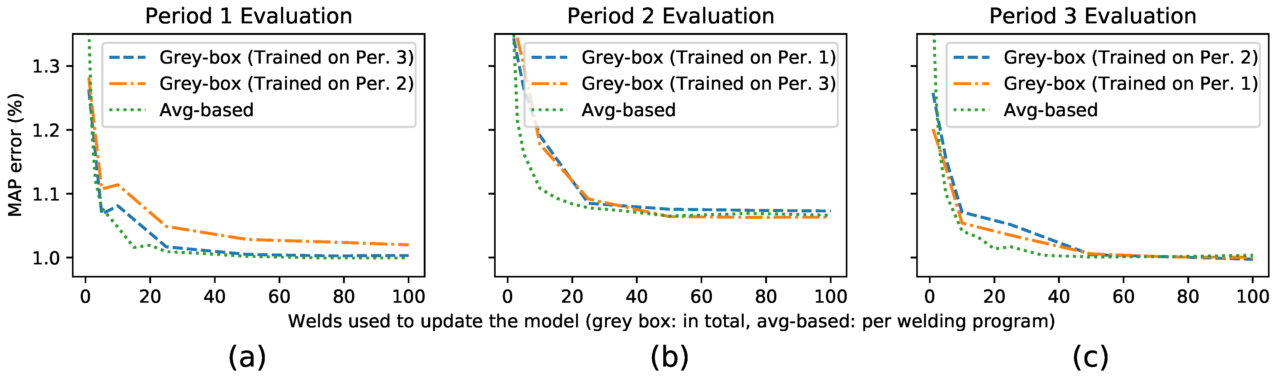
The experiment was performed for all maintenance period combinations, averaging the results of ten different runs. The results are shown in Figure 3, where we see how the grey-box model achieves good predictions using as few as 50 welds to update $R_{mach}$, each time converging to the same error as the average-based model. This confirms that all other grey-box model parameters can be reused across the maintenance periods. The results seem to hint that the average-based model stabilizes using data from fewer welds, but actually, the opposite is true, as the actual weld count should be multiplied by the number of welding programs. It is difficult to determine the number of welds required for reliable predictions when using randomly sampled data due to the welding program imbalance in the data, as the effect on the prediction score will be larger if more commonly used welding programs are sampled. A comparison with a more realistic setting can be made using the experiment in the next section.

We have shown that the grey-box model matches the predictive power of the statistical model while also being interpretable. Next, we demonstrate how the adaptability to changes truly sets the grey-box model apart from the statistical model.

6. Incremental Current Prediction Model

The grey-box model, as discussed so far, would be difficult to implement in a production setting. In the previous experiments, we used the knowledge of the transitions either as a model input or as a trigger to retrain the model, but this is not possible in a real production setting. We could act reactively, i.e., once a transition is suspected, a data scientist would need to confirm this suspicion and retrain the model, and the new model would have to be updated on the process computer. Because such interventions cannot be planned ahead, several days may pass before the model is eventually corrected after a transition. Alternatively, we could periodically retrain the model, though this is somewhat complicated as the predictions are coupled to the process computer, which is not suited for the specialized training process. We will show in this section that local temporal trends are better captured by a dynamic, incremental model. Next, we present a simple approach to update the resistance parameter of our grey-box model in an effective way.

6.1. Updating the Model

Our mechanism to update the resistance parameter is similar to how gradient descent updates the parameters during training. The main difference is that we apply this step per individual data point.

The approach consists of two steps: we determine the value that minimizes the prediction error, and we update $R_{mach}$ towards this value. The first part is straightforward and is shown in Equation (5), which we derive from Equation (3). Here, we use the measured median current I to calculate the ideal machine resistance ${\widehat{R}}_{mach}$, i.e., the value that would have predicted the welding current perfectly.

$$\begin{array}{cc}\hfill {\widehat{R}}_{mach}& =\frac{V_{out}\left(V_{in}\right)}{I}-R_{coil}\left(head\right)-R_{coil}\left(tail\right)\hfill \end{array}$$

(5)

Next, we use ${\widehat{R}}_{mach}$ to update the resistance value in the model using an exponential smoothing function, as shown in Equation (6). Here, $R_{mach}^{\prime }$ represents the updated value, $R_{mach}$ the old value and $\alpha$ is a value in $[0\dots 1]$. By updating the model in this way, we minimize the effect of high-frequency noise while still following the underlying trend. Alternatively, we could use a sliding average over the last N values, but by using exponential smoothing, we effectively put more emphasis on recent values.

$$\begin{array}{cc}\hfill R_{mach}^{\prime }& =(1-\alpha )R_{mach}+\alpha {\widehat{R}}_{mach}\hfill \end{array}$$

(6)

6.2. Evaluation

This last experiment serves to quantify the added value of the incremental grey-box model in a realistic setting. As such, we predict all welds in chronological order, as would be done in a production setting. We assume all welds in the first maintenance period (4679 welds) are available for training purposes and perform a warm-up run for all models by predicting these welds. We only report errors for the welds of periods 2 (9942 welds) and 3 (5289 welds).

All model parameters (except $\alpha$) of the incremental grey-box model were determined during training. After predicting a weld, $R_{mach}$ was updated using the actual measured weld current.

We compare against two incremental versions of the average-based model and an oracle model. The first average-based model (Avg) predicts the welding current as the average of the last N measured welds in the same welding program. The second model (Avg ES) works similarly to the first but uses exponential smoothing to update the prediction value once the model has N historic values for the welding program. We only use exponential smoothing after N values to minimize the effect of noise on the first predictions. Finally, the oracle model is a non-updating version of the physics model that was trained on all of the data of the three periods and tracked a different resistance for each period. This means that the oracle model is evaluated on the same welds it was trained on.

For all models, we calculate the MAP error for all welding currents in periods 2 and 3. To estimate how quickly each model adapts, we also calculate the MAP error when ignoring a predefined number of welds after either transition.

Table 3. Mean absolute percentage error of welding current prediction for all models for all welds in maintenance periods 2 and 3, excluding a number of welds that occur just after either behavioral change. All average-based models perform best when ignoring up to 500 welds after each transition, indicating they require a long time to adjust. In contrast, the physics-based models perform optimally after 50 to 250 welds. Overall, the incremental model outperforms the average-based models and even the oracle model. This shows that welding current is also affected by local temporal changes captured by the incremental model.

	MAP Error (%) Excluding First
Model	X Welds after a Maintenance Period Transition
	0	50	100	250	500
Incr. Grey-box ($\alpha =0.005$)	0.984	0.976	0.968	0.956	0.954
Incr. Grey-box ($\alpha =0.01$)	0.956	0.949	0.944	0.941	0.943
Incr. Grey-box ($\alpha =0.02$)	0.931	0.925	0.923	0.923	0.925
Incr. Grey-box ($\alpha =0.05$)	0.892	0.888	0.887	0.888	0.889
Incr. Grey-box ($\alpha =0.10$)	0.860	0.857	0.856	0.857	0.858
Avg ($N=25$)	1.165	1.160	1.156	1.126	1.094
Avg ($N=50$)	1.263	1.256	1.249	1.215	1.171
Avg ($N=100$)	1.394	1.388	1.379	1.342	1.293
Avg ES ($N=25,\alpha =0.01$)	1.564	1.556	1.548	1.511	1.461
Avg ES ($N=25,\alpha =0.02$)	1.344	1.338	1.330	1.295	1.249
Avg ES ($N=25,\alpha =0.05$)	1.166	1.161	1.156	1.125	1.091
Oracle (Non-Incr. Grey-box)	1.028	1.027	1.026	1.025	1.022

lists the prediction errors and gives several interesting insights.

Looking at both variants of the average-based model, we see better performance when the model can adapt more quickly. This is demonstrated in the first variant (Avg) for the lower window size N and in the second variant (Avg ES) for the higher exponential smoothing factor $\alpha$. Furthermore, we see that all average-based models perform better if we exclude more welds after a transition. This shows that the statistical models would need several days to adjust to the changed behavior.

Looking at the grey-box model, we see better predictions for faster reactivity (higher $\alpha$) but do not see a major improvement beyond skipping 50 to 250 welds. This demonstrates the faster update speed of the incremental model over the average model. The grey-box model clearly outperforms both variants of the average-based model and even the oracle model. The former can be attributed to the shared parameters in the grey-box model, which adjusts the model for all welding programs, whereas the average model has to update each program independently. The latter can be attributed to the fact that the oracle assumes the absence of local trends.

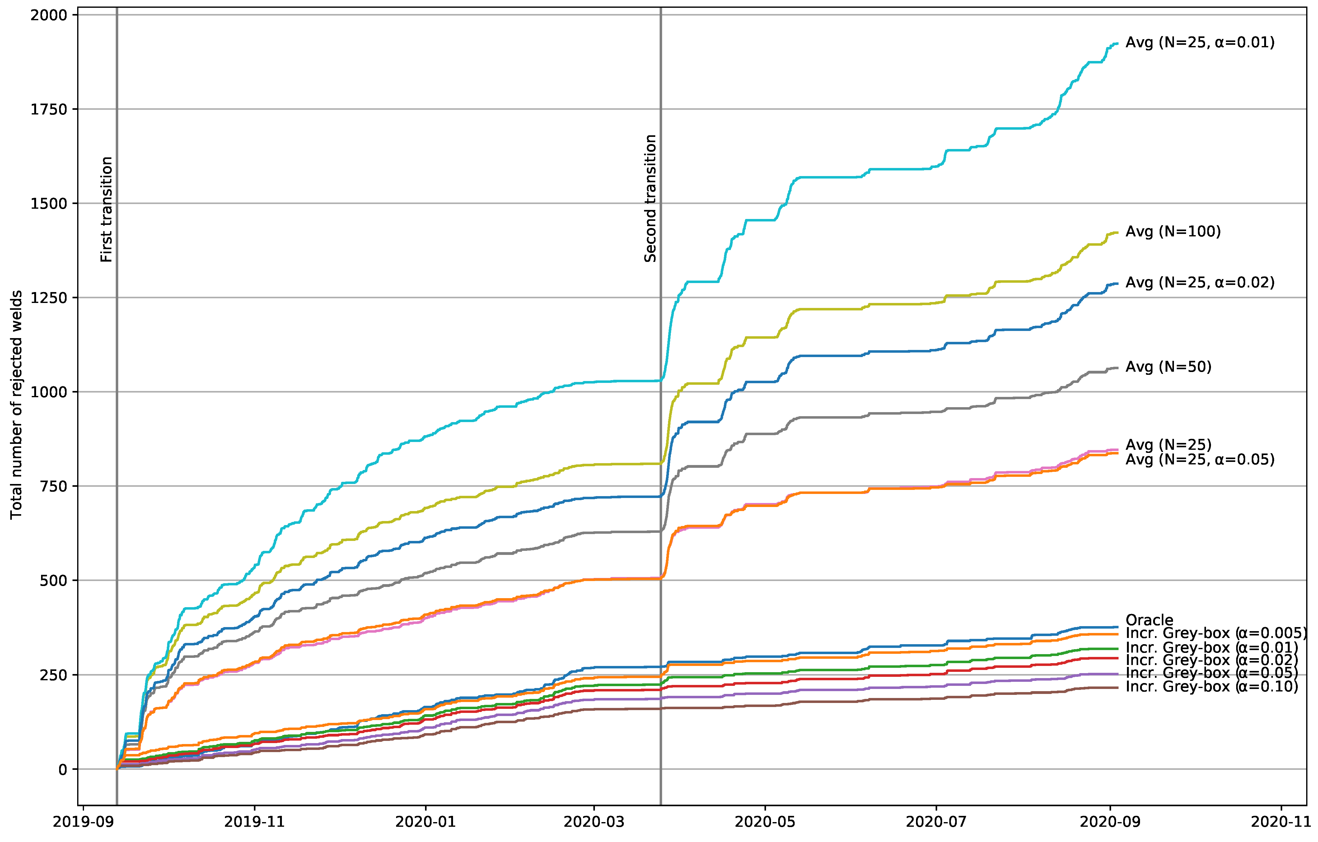
To visualize performance over time, we again define rejected welds as those with a prediction error greater than $3\%$ and plot the total amount of rejected welds over time in Figure 4. We see that despite major differences in the slopes of all models, some general patterns emerge across models, meaning there is a degree of consensus. Overall, the average-based models have more rejected welds. Noticeably, both transitions are followed by a sudden increase in rejections as the average-based models have to update all welding programs. In contrast, the incremental models exhibit only minor jumps after either transition that further diminish for the more adaptive models. Note that small jump artifacts actually may be desired by the operator as a way to notice a behavioral change of the system. In this way, a series of rejected welds over a short period could instigate a further investigation.

All findings point to the presence of both minor and major variations over time of the welding current that is related to the welding machine. The incremental grey-box model is significantly better at keeping up with these changes. In this experiment, the incremental model would have rejected around 250 (1.6%) welds, whereas the best average-based models rejected over 800 welds (5.2%). A process engineer confirmed the benefit of this approach, as it meant that the monitoring system would be less affected by unexpected behavioral shifts while still signaling these shifts.

7. Conclusions

In this work, we detailed the design and evaluation of an incremental grey-box welding current prediction model for the detection of anomalous welds in a steel mill production line. This model displays two major advantages over state-of-the-art statistical models. First, it is possible to model all welding programs in a single unified model, whereas statistical approaches consist of independent models. When external factors change the underlying system, our unified model adapts more efficiently than the independent statistical models. Time and resources will be saved this way, as fewer welds will be incorrectly flagged as anomalous. Secondly, the grey-box model is based on physical laws and can be easily interpreted. This interpretability helps process engineers to trust the model and may lead to additional insights related to the welding process.

Our evaluations utilize 15 months of data collected from the ArcelorMittal Ghent site. The results show that the incremental current prediction model performs better than a non-incremental model (around $0.1$ lower percentage error) and that our model outperforms the statistical models (between $0.1$ and $0.4$ lower percentage error). When using an expert-defined anomaly threshold of three percent, our incremental model results in around two-thirds fewer rejected welds. A non-incremental version of our model performs similarly to the non-incremental statistical model, though our model has the advantage of being interpretable.

Their dependency on physical knowledge forms both the strength and limiting factor of grey-box models. In this work, we achieved good results using commonly-known physical laws, but physics knowledge for other use-cases might be incomplete or not readily available to industry experts. We believe that efficient knowledge exchange between machine learning and physics experts will prove crucial for future success stories.

Various paths for further research remain. In this work, we used an expert-based threshold for classifying anomalies. By using models aware of uncertainty, it could be possible to let the model decide this boundary. Predicting other features, such as temperature, or combining different features into a single anomaly detection model is also an interesting path. Of course, applications need not be limited to the welding domain and can be found for many industry domains. Finally, approaches to create models using incomplete physical knowledge would also have a significant impact.