Different Scales of Medical Data Classification Based on Machine Learning Techniques: A Comparative Study

Abstract

In recent years, medical data have vastly increased due to the continuous generation of digital data. The different forms of medical data, such as reports, textual, numerical, monitoring, and laboratory data generate the so-called medical big data. This paper aims to find the best algorithm which predicts new medical data with high accuracy, since good prediction accuracy is essential in medical fields. To achieve the study’s goal, the best accuracy algorithm and least processing time algorithm are defined through an experiment and comparison of seven different algorithms, including Naïve bayes, linear model, regression, decision tree, random forest, gradient boosted tree, and J48. The conducted experiments have allowed the prediction of new medical big data that reach the algorithm with the best accuracy and processing time. Here, we find that the best accuracy classification algorithm is the random forest with accuracy values of 97.58%, 83.59%, and 90% for heart disease, M-health, and diabetes datasets, respectively. The Naïve bayes has the lowest processing time with values of 0.078, 7.683, and 22.374 s for heart disease, M-health, and diabetes datasets, respectively. In addition, the best result of the experiment is obtained by the combination of the CFS feature selection algorithm with the Random Forest classification algorithm. The results of applying RF with the combination of CFS on the heart disease dataset are as follows: Accuracy of 90%, precision of 83.3%, sensitivity of 100, and consuming time of 3 s. Moreover, the results of applying this combination on the M-health dataset are as follows: Accuracy of 83.59%, precision of 74.3%, sensitivity of 93.1, and consuming time of 13.481 s. Furthermore, the results on the diabetes dataset are as follows: Accuracy of 97.58%, precision of 86.39%, sensitivity of 97.14, and consuming time of 56.508 s.

1. Introduction

The rapid increase in digital data has enabled the generation of medical big data. Data analysis is an important tool, paving the way towards achieving accuracy of big medical data [1]. Machine learning techniques, in particular, traditional data mining techniques are used to raise the accuracy and efficiency of medical data analysis. Due to the large size of the data, these techniques are not suitable for collecting, storing, and analyzing these datasets [2]. In medical data mining, for example, consultants prepare reports regarding their patients in order to give an accurate and efficient decision on their patients’ health. This discovered information is available for consultants and patients to access in order to reach an accurate diagnosis [3,4].

The high volume of medical data and rapid advances in this field have resulted in the so-called medical big data. Medical big data have large datasets and do not fit into traditional database architectures. They require different techniques, tools, and architectures to deal with past and recent challenges in more effective ways [5]. One way of dealing with these challenges is through accurate decisions. Machine learning algorithms, which are more frequently used, overcome these challenges by extracting knowledge and reaching new patterns, rather than simply accessing information [6]. In the medical field, the choice of an effective machine learning algorithm is a critical issue, since each algorithm has an impact on the accuracy of the result. No one algorithm works best for all issues, due to the fact that each algorithm has its own characteristics. The most commonly used machine learning algorithms in mechanical engineering can be separated into the following classes: Regression, estimation, classification, and clustering. Specifically, the regression or classification algorithms operate for a significant prediction [7]. The application of big data analytics in healthcare is important for several reasons [8]:

• Continuous detection of the patient’s health and state. In the case of an unusual event, an alarm is sent to the patient’s doctor for an early intervention.
• Early detection of disease.
• Prediction of new disease.

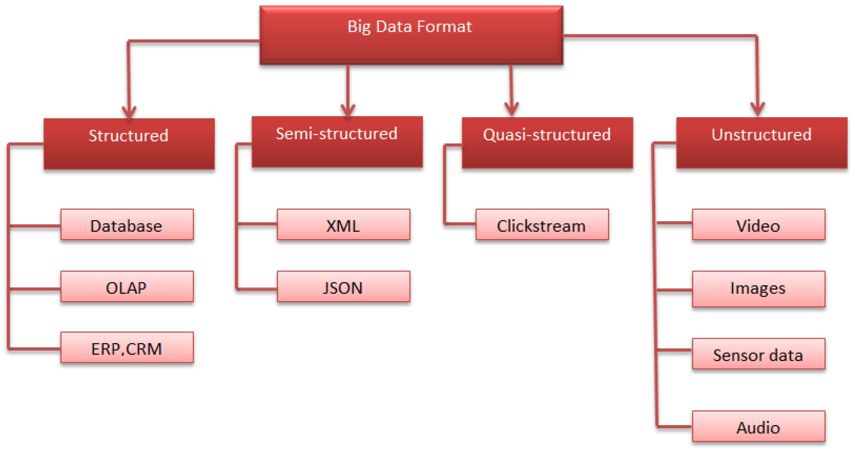
Different formats of big data are shown in Figure 1. Big data is composed of four diverse data formats, including structured, semi-structured, quasi-structured, and unstructured data formats.

Challenges of Big Data in Healthcare

Nowadays, the significance of big data analytics lies in raising and evaluating the application of big data analytics in the larger prescriptive. Therefore, it is important to outline some challenges of big data applications in healthcare. There are many methodological issues, such as data quality, data inconsistency, validation, and analytical issues. In addition, there is a need to enhance the data quality of electronic health records [9]. In the medical field, although disease prediction is one of the essential areas of research, the codes are not assigned in many databases. Therefore, these values need to be corrected. Another challenge is clinical integration. Big data analytics need to be integrated into a database to obtain significant advantages, and clinical integration needs the validation of big data analytics. It is important to solve these challenges to enhance the quality of big data application in the medical field. This improves patient outcome and reduces the waste of resources in healthcare, which should be the real value of big data studies [10].

Medical big data faces many challenges, as follows [11]:

• Collecting patient data continuously from different sources, thus leading to the high volume of data.
• Medical data are almost unstructured or semi-structured.
• Medical data are not clear for everyone.
• Handling a huge size of medical data.
• Extracting useful information from medical big data.

The objective of this paper is to provide a comprehensive review of the implementing models of the state of art, and to present a comparative analysis of the seven different algorithms, which are mostly implemented in previous works. Here, we compare these seven algorithms on different datasets in order to evaluate the accuracy of each algorithm and conclude the best algorithm with the highest accuracy.

In this paper, machine learning methods are used to predict different diseases from new emerging data. Seven algorithms are tested and enhanced using the CFS feature selection algorithm to achieve better accuracy in the prediction stage. Then, we compare these algorithms’ results for the heart disease dataset and repeat this comparison for the M-health and diabetes datasets.

The rest of this paper is structured as follows: Section 2 explains the related work of medical big data, while Section 3 presents the basic concepts which are used for the experiments. Section 4 describes the proposed model and its steps. Section 5 discusses the results of our experiments, and finally Section 6 presents the conclusions and future work.

2. Related Work

Medical big data classification and prediction are an important issue. In recent years, many researchers have made significant efforts to increase the benefits of these data. Utilizing an experiment, Gavai et al. [12] investigated the ability to detect which regions of the country have an increase in disease. To perform the experiment, ontologies were used and revealed that 62% of the patient population had the disease. For a new population percentage, this investigation should be replicated on different patients.

Other researchers utilized the LR and RF algorithms to predict new data. The first research used LR with the principal component analysis (PCA). In this case, Ansari et al. [13] applied a model using UCI machine learning repository datasets to forecast whether a person has heart disease. Initially, the authors trained LR with all of the attributes. Then, they trained LR after removing the least significant attributes and suggested a model, which is LR with PCA. Finally, LR with PCA achieved the best accuracy of 86%. The results obtained determine whether heart disease exists with different levels of presence.

Singh et al. [14] suggested medical services that are suitable for everyone. The authors predicted liver disease depending on a classification algorithm technique using the feature selection method. The experiments were conducted based on the Indian liver patient dataset (ILPD) from the database of University of California, Irvine. The different attributes of the dataset are important to predict the risk level of disease. Various classification algorithms, such as LR, SMO, RF, NB, J48, and KNN were used to evaluate the accuracy. Here, both a comparison of different classifier results and the development of an intelligent liver disease prediction software (ILDPS) were performed using the feature selection and classification prediction techniques, based on a software engineering model. The best accuracy value is 77.4% for the LR algorithm with feature selection techniques. In this context, we suggest the use of the CFS algorithm for feature selection to enhance the accuracy value.

Another research by Kondababu et al. [15] applied LR with RF to predict heart disease. The authors used the UCI heart disease dataset to predict heart disease in its early stages for disease control. A comparative analysis was conducted using different classification algorithms. The best accuracy value is 88.4% for RF with LM. In this context, we suggest the use of suitable data preprocessing steps to enhance the accuracy value.

Numerous researchers applied the RF, KNN, SVM, NB, and R algorithms on their own or with another algorithm for the classification of new data. Ali et al. [16] applied many supervised machine learning algorithms and compared them to evaluate the accuracy in heart disease prediction. Importance scores for each feature were estimated for all of the applied algorithms, except for MLP and KNN. All of the features were classified based on the importance scores, such as accuracy, precision, and sensitivity to find the highest heart disease prediction. The authors used a heart disease dataset from Kaggle, and implemented the MLP, DT, KNN, and RF algorithms. Three classifications based on the KNN, DT, and RF algorithms have the highest accuracy value. The RF method was conducted with 100% sensitivity and specificity. Therefore, a relatively simple and supervised machine learning algorithm can be used for heart disease prediction, with very high accuracy and excellent potential utility.

Subasi et al. [17] proposed a model using the M-health dataset. The results showed that the proposed model with the RF and SVM classification algorithms have the highest accuracy and are highly effective. The RF algorithm is most efficient with a high amount of data, and thus results in a high accuracy value.

Jan et al. [18] implemented a data mining method using two standard datasets, which were obtained from the UCI repository, namely Cleveland and Hungarian. The authors experimented with five different classification algorithms, such as RF, NN, NB, R, and SVM. They concluded that the lowest-performing algorithm was the regression classification, while RF had a very high accuracy of 98.136%. The regression algorithm had the lowest accuracy value with a high volume of data.

Khan et al. [19] experimented with the Naïve bayes (NB) algorithm. The authors concluded that the accuracy changed with the increase of data. When the data increased, the accuracy of the model decreased. In this experiment, the NB method achieved a 98.7% accuracy. Moreover, it is suitable for small datasets. Therefore, other algorithms should be experimented for a good accuracy value.

Mercaldo et al. [20] proposed a method that classified the dataset into diabetes-affected patients and not affected ones using classification algorithms. The authors evaluated their model on real-world data, which were obtained from the Pima Indian population. They trained the model using six various algorithms, such as J48, MLP, HoeffdingTree, JRip, Bayes Net, and RF, and obtained a precision equal to 0.757 and a recall of 0.762. Although various algorithms were used, no single algorithm provided a sufficient accuracy value. In this context, experiments with new classification algorithms are required to provide high accuracy.

The following researches implemented the DT algorithm for classification. Jothi et al. [21] tested the data using the python programming language. The output of the program displayed the risks of having heart disease. The authors used the DT and KNN algorithms for heart disease prediction. The DT algorithm tested the dataset to predict the chances of having heart disease and had an accuracy rate of 81%. In addition, the KNN algorithm tested the same dataset and had an accuracy rate or level of 67%. In the proposed work, we assume that the RF algorithm is more efficient, can be used for the automated work analysis, and enhances the accuracy value of work. Moreover, Arumugam et al. [22] predicted diabetes-related heart disease, which is a kind of heart disease that affects diabetic people. Heart disease refers to a set of conditions that affect the heart or blood vessels. Although various data mining classification algorithms exist for heart disease prediction, there is inadequate data for heart disease prediction in a diabetic individual. Three different algorithms were implemented, including NB, SVM, and DT. Of note, the DT model consistently had higher accuracy than the NB and SVM models, with a 90% accuracy value.

In the research by Pinto et al. [23], the J48 algorithm was used based on the chronic kidney disease (CKD) dataset. The CKD is categorized into various degrees of risk using standard markers. It is usually asymptomatic in its early stages, and early detection is important to reduce future risks. This study experimented with the cross industry standard process for data mining (CRISP-DM) methodology and the WEKA software to develop a system that can categorize the chronic condition of the kidney, depending on accuracy, sensitivity, specificity, and precision. The J48 algorithm provided the following results: 97.66% of accuracy, 96.13% of sensitivity, 98.78% of specificity, and 98.31% of precision.

The following research by Mateo et al. [24] implemented the GBT algorithm. The authors predicted acute bronchiolitis for new children. The selection of suitable treatments is significant for disease progress. An extreme gradient boosting (XGB) classification algorithm, which is a machine learning method that is suggested in this paper, was used for medical treatment prediction. Four supervised machine learning algorithms incorporating KNN, DT, NB, and SVM were compared with the suggested XGB method. The results showed that the XGB had the highest prediction accuracy of 94%. In this context, the implementation of data reduction techniques is important to enhance prediction accuracy.

In this paper, various classifier techniques are proposed that involve a combination of machine learning algorithms with a feature reduction algorithm to detect the redundant features and enhance the accuracy and quality of heart disease, m- health, and diabetes disease classification. Here, we present an evaluation for various disease classifications using seven algorithms. Then, we study the performance of NB, LM, R, DT, RF, GBT, and J48 classifiers. The main goal of this research is to find the best accuracy for the prediction of different diseases using major factors based on different classifier algorithms. The use of CFS algorithm with a combination of classification algorithms provides a better accuracy value in comparison with the results of the literature works.

Table 1. Comparison between different research studies on medical data.

Reference	Year	Dataset	Algorithm	Accuracy	Advantages/Disadvantages
Khan et al. [19]	2016	Adult	NB, C4.5	98.7%	The accuracy changed with the increase of data. When the data increased, the accuracy of the model decreased. NB is good with a small dataset.
Mercaldo et al. [20]	2017	Diabetes Pima Indian	J48, MLP, Hoeffding Tree, JRip, Bayes Net, RF	77.6%	They used various algorithms but no single algorithm provided a sufficient accuracy value. They need to experiment with new classification algorithms which provide high accuracy.
Subasi et al. [17]	2018	M-health	SVM, RF	86%	The RF algorithm is most efficient with a high amount of data. It results in a high accuracy value.
Jan et al. [18]	2018	Cleveland and Hungarian.	RF, NB, R, NN, SVM	98.136%	While RF provides very high accuracy, the regression algorithm provides the lowest accuracy value with a high volume of data.
Singh et al. [14]	2020	Indian Liver Patient Dataset (ILPD)	LR, SMO, RF, NB, J48, IBk	77.4%	The best accuracy result was from the LR with feature selection. We suggest using the CFS algorithm for feature selection to enhance the accuracy value.
Pinto et al. [23]	2020	Chronic Kidney Disease	J48	97.66%	They developed a system that can categorize the chronic condition of kidney diseases. The J48 algorithm is suitable for the small or medium volume of data.
Ansari et al. [13]	2020	UCI Heart Disease	LR, PCA	86%	LR with PCA achieved the best accuracy.
Ali et al. [16]	2021	Kaggle Heart Disease	MLP, RF, DT, KNN	100%	Three classifications based on KNN, DT, and RF algorithms have the highest accuracy value.
Jothi et al. [21]	2021	Heart Disease	DT, KNN	81%	DT has 81% accuracy and the KNN algorithm has an accuracy rate or level of 67%. We assume that the Random Forest algorithm is more efficient with the proposed work.
Arumugam et al. [22]	2021	Diabetes based Heart Disease	NB, SVM, DT	90%	DT has the highest accuracy value. The DT model consistently has higher accuracy than NB and SVM models.
Mateo et al. [24]	2021	Acute Bronchiolitis	GBT, KNN, NB, SVM, DT	94%	The XGB has the highest prediction accuracy. Reduction data implementation is important to enhance the accuracy value of the prediction.
Kondababu et al. [15]	2021	UCI Heart Disease	RF, LM	88.4%	We suggest the use of suitable data preprocessing steps and a reduction algorithm as the CFS to enhance the accuracy value.

shows the comparison between different research studies on medical data. It presents the implemented algorithms and accuracy results, as well as the advantages and disadvantages of each work.

3. Methodology

3.1. DT

Decision tree (DT) is a hierarchical division of the data and an algorithm for decision support. It is similar to a flowchart, in which each internal node represents a test attribute, the endpoint is a response or the class label, and each branch represents the classification rule [25,26]. The following parameters are used to improve the performance of decision tree:

• The max_depth parameter represents the maximum depth of the tree. Without defining this parameter, the tree can lead to an infinite loop until all of the leaves are expanded. We assign it as 20.
• The criterion parameter represents the measure of the split’s quality. Here, we use entropy, which measures the information gain.

  $$\mathit{E}\mathit{n}\mathit{t}\mathit{r}\mathit{o}\mathit{p}\mathit{y}={\displaystyle \sum }_{\mathit{i}=\mathbf{0}}^{\mathit{n}}\mathit{p}\mathit{i} {\mathit{l}\mathit{o}\mathit{g}}_{\mathbf{2}} \mathit{p}\mathit{i}$$

  (1)

Information gain is a measure used for segmentation and is known as mutual information [27]. This denotes the amount of knowledge needed for a variable’s value. It is the opposite of entropy, where the higher the value, the better. In the definition of entropy, data gain (S, A) is defined as shown in Equation (2):

$$Gain={\displaystyle \sum }_{i=1}^n\left(\frac{\left|\mathrm{sv}\right|}{\left|\mathrm{v}\right|}\right) entropy \left(s\right)$$

(2)

where the range of attribute A is (A), and Sv is a subset of set S, which is equal to the attribute value of v.

3.2. RF

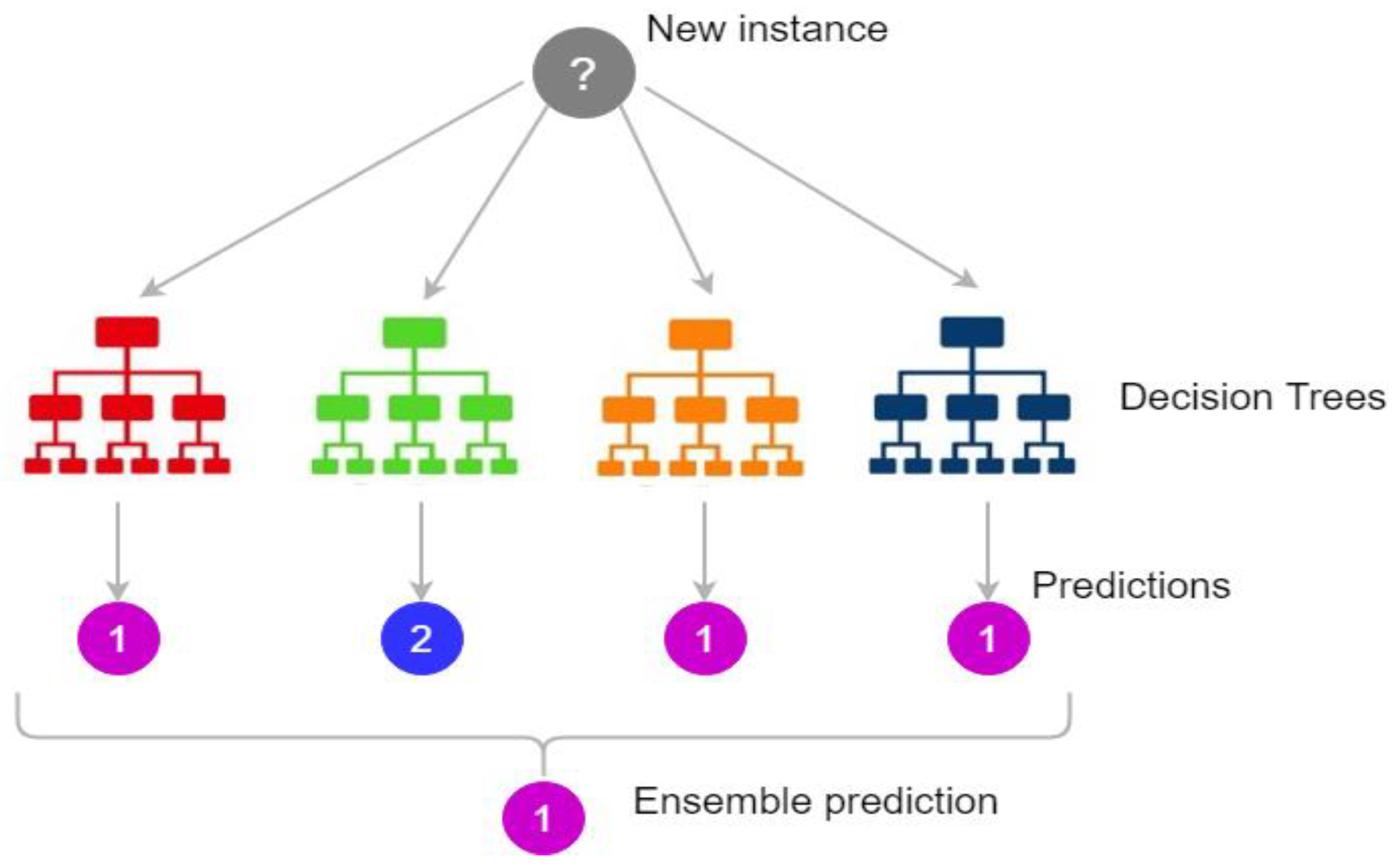
Random forest (RF) is a real-time ensemble classification algorithm. It is composed of a set of trees, with each tree depending on random variables. The vector X = (X₁, X₂…, X_n)^T represents the input value, the random variable Y represents the response or prediction values, and the used joint distribution is PXY (X, Y). The goal is predicting Y from a prediction function f(X) [28].

The class prediction is conducted by the majority of votes, which is defined as the most common class prediction between trees. Therefore, the voting occurs on the class probability level. The predictions select the class with the highest class probability as shown in Figure 2.

Figure 2 shows how the ensemble classification done. It gathers the results from different trees and votes the results then it chose the result with the highest voting.

The following parameters are used to enhance the classification accuracy:

• The n_estimators’ parameter represents the number of trees that we need to build prior to voting. Better accuracy results from the highest number of trees, but it results in high-performance time. We use 50 tree numbers for an efficient classification.
• The max_depth parameter represents the maximum length of the trees. If we do not assign a value for max_depth, it may lead to infinite nodes. We assign it as 20.

3.3. J48

The J48 is a tree-based algorithm, which is used to discover the way the attribute vector performs for a number of instances. Moreover, on the basis of the training instances, the classes for the newly produced data are found. This algorithm produced the rules for the outcome variable prediction. With the aid of tree classification algorithm, the correct distribution of the data is easily reasonable. J48 is an expansion of ID3. The additional features of J48 include calculating the missing values, decision trees pruning, continuous attribute value ranges, etc. The J48 is an open source Java implementation of the C4.5 algorithm. It presents a set of options related to tree pruning. In the case of potential over fitting, pruning can be used as a precision tool [30].

For other algorithms, the classification is achieved recursively until every single leaf is pure. In this case, the classification of the data should be as precise as possible. The J48 generates the rules from which a specific identity of the data is produced.

3.4. LM

The linear model (LM) expands the concept of the well-known linear regression model. It simplifies the linear regression by permitting the linear model to be associated to the response variable via a link function and by permitting the significance of the variance of every measurement to be a task of its predicted value. It offers an iteratively reweighted least squares method for maximum likelihood approximation of the parameters. Maximum likelihood approximation has become more common and is the standard way on most statistical computing packages [31]. Other approaches, incorporating Bayesian methodologies and least squares fits to variance responses, have been improved.

3.5. R

Logistic regression (R) is a statistical tool used in the medical field. Logistic regression adds a coefficient to each predictor. The Y variable takes the (1) value if the label is yes and takes the (0) value if the label is no. If the label has two values, the binary logistic regression is used. However, in the case of more than two values, the multinomial logistic regression is used [32].

The following parameters and attributes are used for accuracy enhancement:

• The max_iter parameter represents the maximum number of iterations until it converges. We assign it as 20.
• The random_state parameter represents the random values used in shuffling.
• The classes attribute represents the list of class labels for a clear classification.

3.6. GBT

The gradient boosted tree (GBT) is a very common supervised learning approach, which is used in medical areas. In addition to high accuracy, this approach quickly predicts new values and has a small memory foot print. GBT training for huge datasets is challenging even with extremely optimized packages, such as XGBoost. Moreover, it is not possible to continuously upgrade GBDT models with new data [33].

The following parameters are used for accuracy enhancement:

• The max_depth parameter represents the maximum length of the trees. If we do not assign a value for max_depth, it may lead to infinite nodes. We assign it as 20.
• The learning rate presented is assigned to 0.01.

3.7. NB

Naïve bayes (NB) is a classification algorithm that produces a likelihood of a specific set of explanations related to a specific class [34], which differ due to the values of the class label variable. The NB classifier has been accepted as a basic probabilistic classifier, which relies on clear independent principles of Bayesian theorem [35].

In machine learning and data mining, classification is a basic issue. In a classification, the concept of this algorithm is to construct a classifier with class labels. The NB approach is a supervised classification algorithm which uses the theorem of Bayes [36].

3.8. CFS

Correlation feature selection (CFS) is an essential step of the preprocessing phase in the process of classification and prediction. Attribute selection, variable selection, feature construction, and feature extraction are the different names assigned to feature selection algorithms. They are mainly used for data reduction by eliminating unrelated and redundant data. Feature selection enhances the characteristics of the data and raises the accuracy of classification algorithms by decreasing the data volume and processing time [30]. There are many feature selection algorithms, such as principal component analysis (PCA), singular value decomposition (SVD), CFS, etc. The most effective feature selection algorithm with our data is the CFS. It is suitable for our data parameters, which are numerical and textual data. In addition, CFS can improve the classification accuracy and efficiency by removing redundant features.

4. Comparison between Medical Data Classification Methods

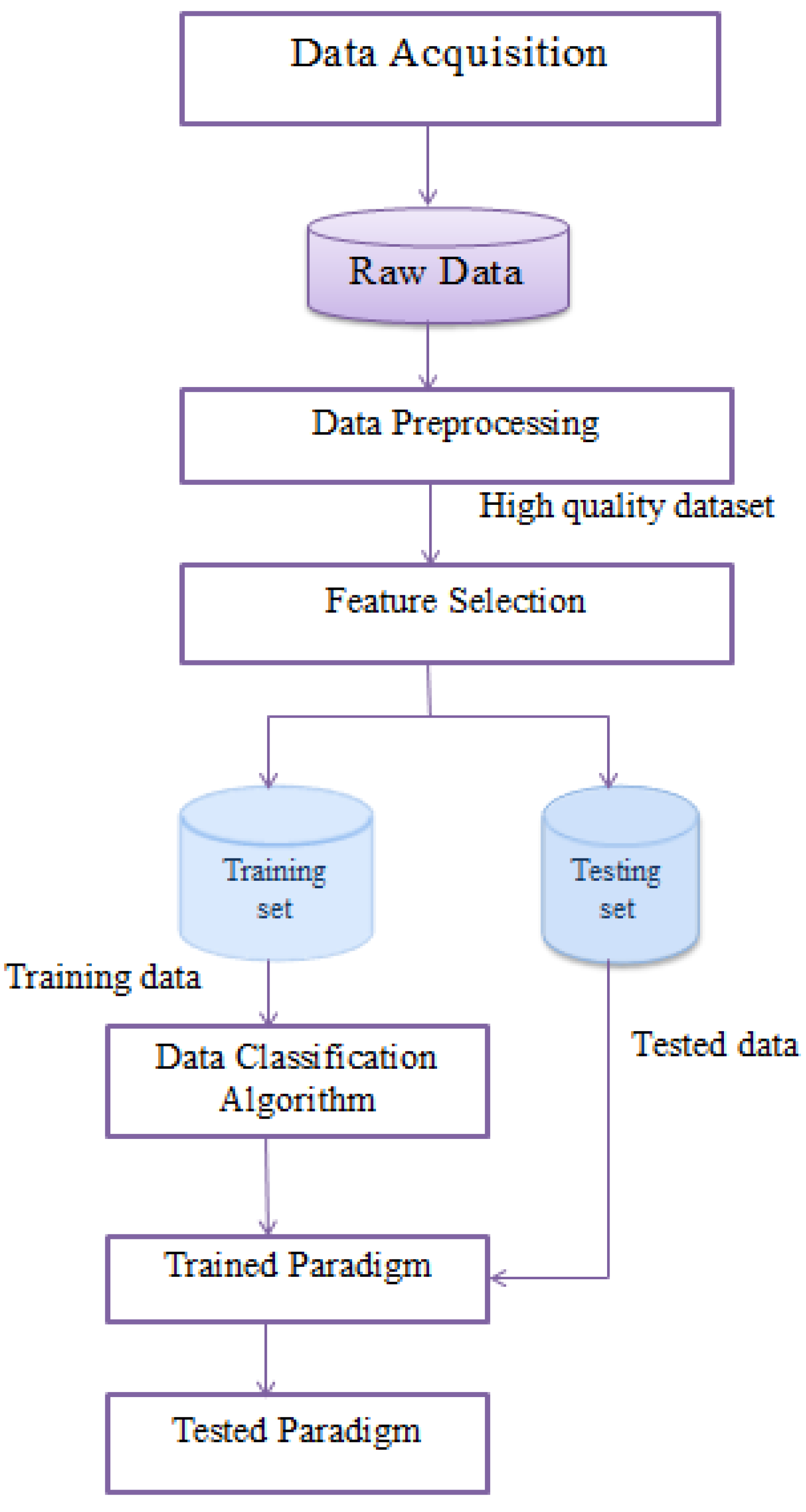
The prediction of new data from big medical data is not an easy challenge. There are many algorithms used for classification or prediction. In this paper, we implemented them on medical big data using seven different classification algorithms to identify the best algorithm with the highest accuracy and lowest processing time. The classification algorithms do not reach a good accuracy on their own; they require preprocessing steps to enhance the data quality. To enhance the accuracy, preprocessing steps and the feature selection method were used. The preprocessing steps clean the data from noise and replace the missing data. The feature selection method allows the reduction of the data structure, which affects the accuracy and running time of the prediction step. These steps are explained in Figure 3.

Data processing has major advantages. However, it also has many disadvantages, as follows:

• Machine learning needs to train on huge datasets, and these should be unbiased as well as of good quality. As a result, there can be periods where we should wait for new data to be produced.
• Sufficient time is required for the algorithms to learn how to achieve their purpose with accuracy. Machine learning also requires massive resources to function, which leads to additional computer power requirements [37].

From a data mining perspective, medical data classification is a process that requires the following main steps: (I) Data acquisition, (II) data preprocessing, (III) feature extraction, and (IV) data classification. Figure 3 shows the steps of preprocessing, feature selection, and classification. In the following sub-sections, we discuss these steps.

I.

Data Acquisition

Raw data are obtained from different sources since we use three different datasets. Then, to understand the data, we review the dataset attributes, values, and instances.

II.

Data Preprocessing

Raw data have many challenges due to the continuous collection of data from different medical sources. The analysis of this data results in a low accuracy value with inaccurate prediction results. The three datasets used have many redundant values and a set of missing data. Therefore, in this step, we clean the dataset by removing duplications and replacing the missing data with the “Unknown” value for categorical data and the mean value for the numerical data. The output of this step is a clean and high-quality dataset, which increases the accuracy of the used algorithms.

III.

Feature Selection

Data selection is conducted by finding standard features of data, which represent the original data. The featured dataset is the input of the classification step, rather than the full data. The feature selection step is one of the most important steps. It reduces data by focusing on the featured data. There are many feature selection algorithms, such as principal component analysis (PCA), singular value decomposition (SVD), CFS, etc. The most effective feature selection algorithm with our data is the CFS. It is suitable for our data parameters, which are numerical and textual data. CFS can improve the classification accuracy and efficiency by removing redundant features. Let X be the set of all the features of the dataset with a large number of features {f₁, f₂, f₃, …, f_n}, where n is the number of the attributes or features of the dataset. The feature selection process involves selecting the data, which generates × set of features with a small number of features [38].

IV.

Data Classification

Data classification has two stages, which are the training stage and the testing stage. In the training stage, part of the preprocessed data, which is 70%, is inputted into a defined classification algorithm that generates a training model. Then, in the testing stage, the other part of the preprocessed data, which is 30%, is inputted into the tested model to evaluate the defined classification algorithm. Seven classification algorithms, which are NB, LM, R, DT, RF, GBT, and J48 are implemented on our data.

5. Results and Discussion

In this work, various techniques were implemented on three datasets [39,40,41]: Radoop, Waikato (Weka 3.9), and MATLAB 2020a. The experiments were implemented on a computational server with the following specifications: Windows 10 64-bit operating system, with processor Intel(R) 16 GB of RAM Core (TM) i7-7500U CPU @ 2.70 GHZ 2.90 GHz. In all cases, the implementation has been conducted in parallel.

5.1. Dataset Description

Table 2. Description of the three experimented datasets.

Dataset	Attributes’ Number	Instances’ Number	Missing Data (Y/N)	Redundancy (Y/N)	Noise (Y/N)
M-Health [39]	24	161281	Y	Y	Y
Diabetes [40]	50	101797	Y	Y	N
Heart Disease [41]	19	59077	Y	N	Y

shows the properties of the three experimented datasets. It presents the number of attributes and instances as well as whether there are missing data, redundancy, and noise.

Table 3. Characteristics of the three datasets after preprocessing and feature selection.

Dataset	Encoding (Y/N)	Feature Selection (Y/N)	Attributes’ Number
M-Health	N	Y	12
Diabetes	Y	Y	29
Heart Disease	Y	Y	10

shows the characteristics of the different datasets after the preprocessing step. It presents whether the data are encoded, whether the set of attributes required an implementation of feature selection, as well as the number of attributes after the feature selection step.

5.2. Results

Table 4. Comparison between different algorithms applied on heart disease data without preprocessing.

Algorithm	Accuracy	Relative Error	Precision	Sensitivity	Time (s)
NB	66.2	33.8	75.2	89.56	1.39
LM	69.96	30.04	70.43	72.67	3.9
R	74.4	25.6	69.73	70.02	8.04
DT	75	25	78.43	78.9	4.7
RF	75.2	24.8	89.52	99.06	9.12
GBT	74.1	25.9	87.4	90.02	16.79
J48	72.9	27.1	70.42	84.1	86.83

,

Table 5. Comparison between different algorithms applied on preprocessed heart disease data.

Algorithm	Accuracy	Relative Error	Precision	Sensitivity	Time (s)
NB	77.5	22.5	86.7	65	0.078
LM	82.5	17.5	78.3	90	3
R	90	10	86.4	95	2.95
DT	80	20	73.1	95	2.99
RF	90	10	83.3	100	3
GBT	90	10	83.3	100	16
J48	84.56	15.44	84.6	84.6	85.5

and

Table 6. Comparison between different algorithms applied on M-health data without preprocessing.

Algorithm	Accuracy	Relative Error	Precision	Sensitivity	Time (s)
NB	70.82	29.18	68.75	74.15	9.07
LM	65.67	34.33	72.36	71.08	12.08
R	70.39	29.61	68.87	69.17	10
DT	70.04	29.96	79.6	76.75	12.613
RF	79.2	20.8	75.46	80.05	16.814
GBT	74.25	27.75	76.21	77.8	685.47
J48	60.4	39.6	65.8	60.7	91.65

show the comparison between different classification algorithms, such as NB, LM, R, DT, RF, GBT, and J48. The classification algorithms are tested with preprocessing data cleaning steps, such as duplication and missing data removal. The processing time for executing the tested algorithms on diabetes data is increased, compared to the other tested datasets. Whereas the data volume increased, the running time of algorithms increased, as shown in Table 6.

The experiments were evaluated using three datasets: Heart disease, M-health, and diabetes datasets. The classification algorithms were experimented by the Raddoop platform and MATLAB 2020a. In addition, the preprocessing and CFS reduction algorithms were implemented by the Waikato platform (Weka 3.9). Moreover, the classification algorithms were tested before and after applying the preprocessing step. From our studies, we conclude that the application of data reduction decreases the consuming time and preprocessing enhances the quality of the data, which lead to a better accuracy value.

Table 4 and Table 5 show the comparison between different classification algorithms on the heart disease dataset before and after applying preprocessing on the data. The tables present the accuracy, relative error, precision, sensitivity, and time of each algorithm. The mathematical analysis of error calculation is a critical portion of the measurement. This analysis detects the actual value and the error quantity. The relative error conducts how good or bad the classification is. In mathematical measurements, the errors are conducted by a round-off error or truncation error.

In Table 4 and Table 5, the results show that the accuracy after preprocessing is better than without preprocessing for all of the tested algorithms. Moreover, regarding time processing, the time processing of the algorithms without preprocessing is longer than the time processing of the preprocessed data.

In Table 5, the results show that in the heart disease dataset, the J48 algorithm takes a long time for processing with 85.5 s. In addition, the NB algorithm takes the lowest processing time with 0.078 s, but it has a minimum accuracy value of 77.5%. Moreover, the highest accuracy is the same for R, RF, and GBT with a 90% value.

Table 6 and

Table 7. Comparison between different algorithms applied on preprocessed M-health data.

Algorithm	Accuracy	Relative Error	Precision	Sensitivity	Time (s)
NB	82.25	17.75	88.2	70.04	7.683
LM	70.44	29.65	74.31	82.52	10.158
R	77.1	22.9	81.1	89	9.351
DT	79.04	20.96	66.23	90.2	9.926
RF	83.59	16.41	74.3	93.1	13.481
GBT	79.29	20.71	72.13	91.4	446.8
J48	66.39	33.61	61.2	54.2	72.42

show the comparison between different classification algorithms on the general health (M-health) dataset before and after preprocessing. The tables present the accuracy, relative error, precision, sensitivity, and time of each algorithm.

In Table 6 and Table 7, the results show that the accuracy after preprocessing is better than without preprocessing for all of the tested algorithms. Moreover, for time processing, the time processing of the algorithms without preprocessing is longer than the time processing of the preprocessed data.

In Table 7, the results show that in the M-health dataset, when the data increases, the accuracy of R and GBT decreases. The best accuracy is 83.59% for the RF algorithm, but the low accuracy value is 66.39% for the J48 algorithm. The lowest processing time is 7.683 s for the NB algorithm, but the highest processing time is 44.68 s for the GBT algorithm.

Table 8. Comparison between different algorithms applied on diabetes data without preprocessing.

Algorithm	Accuracy	Relative Error	Precision	Sensitivity	Time (s)
NB	93.62	6.38	87.9	90.18	27.026
LM	91.73	8.27	81.6	83.6	31.4231
R	80.09	19.91	68.06	74.5	31.753
DT	92.53	7.47	85.5	89.086	33.9
RF	93.96	6.04	90.26	91.47	58.205
GBT	91.07	8.93	89.69	87.05	123.45
J48	70.23	29.77	70.1	72.06	90.64

and

Table 9. Comparison between different algorithms applied on preprocessed diabetes data.

Algorithm	Accuracy	Relative Error	Precision	Sensitivity	Time (s)
NB	96.16	3.84	83.35	91.43	22.374
LM	94.4	5.6	81.03	76.98	26.564
R	85.31	14.96	79.01	95	29.064
DT	96.85	3.15	85.8	95.48	33.667
RF	97.58	2.42	86.39	97.14	56.508
GBT	96.55	3.45	85.08	95.08	117.845
J48	73.828	26.172	73.5	75.1	87.24

show the comparison between different classification algorithms on the diabetes dataset before and after preprocessing. The tables present the accuracy, relative error, precision, sensitivity, and time of each algorithm.

In Table 8 and Table 9, the results show that the accuracy after preprocessing is better than without preprocessing for all of the tested algorithms. Moreover, for time processing, the time processing of the algorithms without preprocessing is longer than the time processing of the preprocessed data.

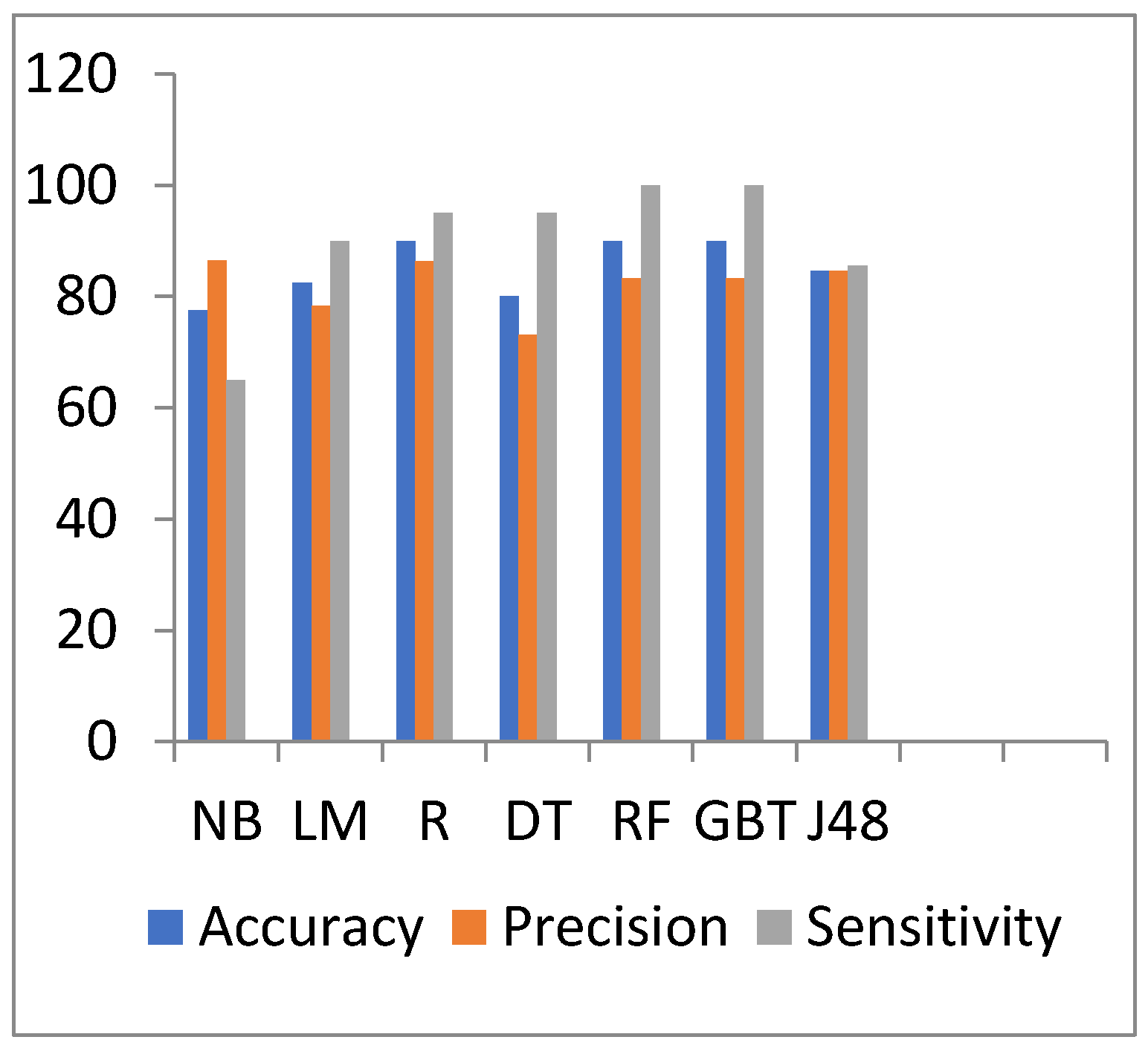
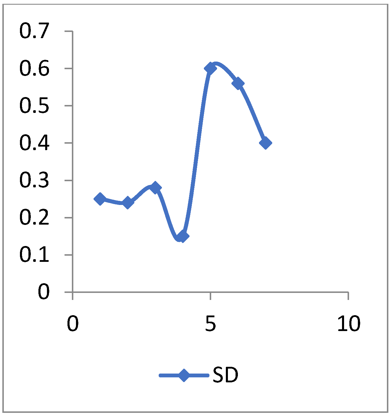
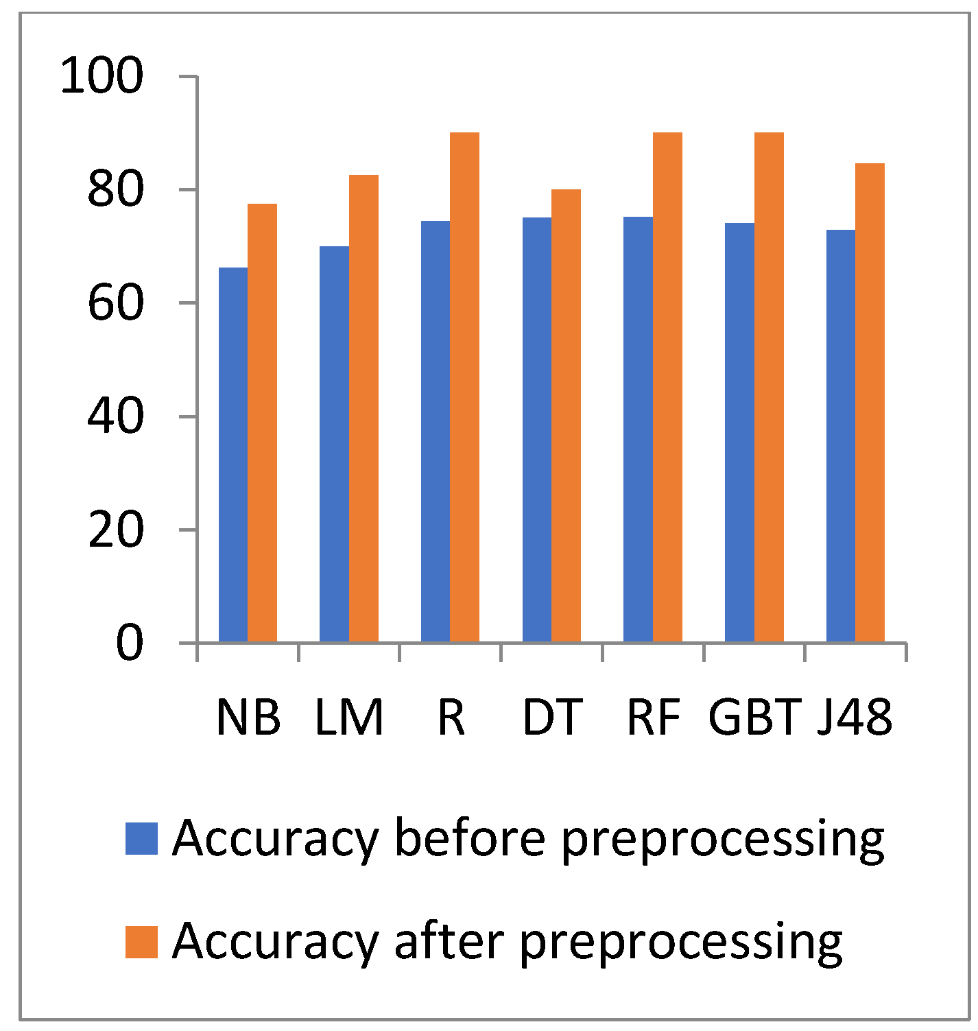
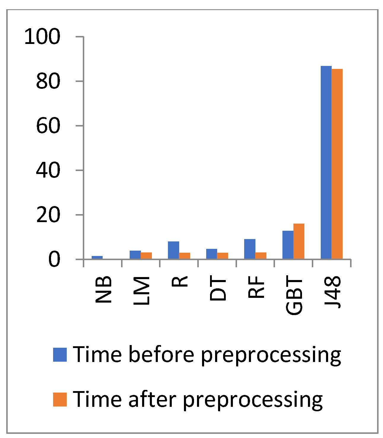
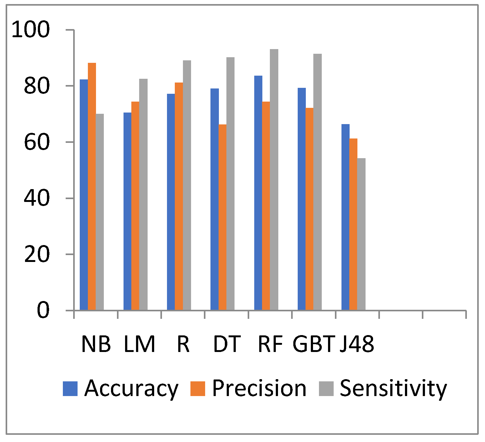
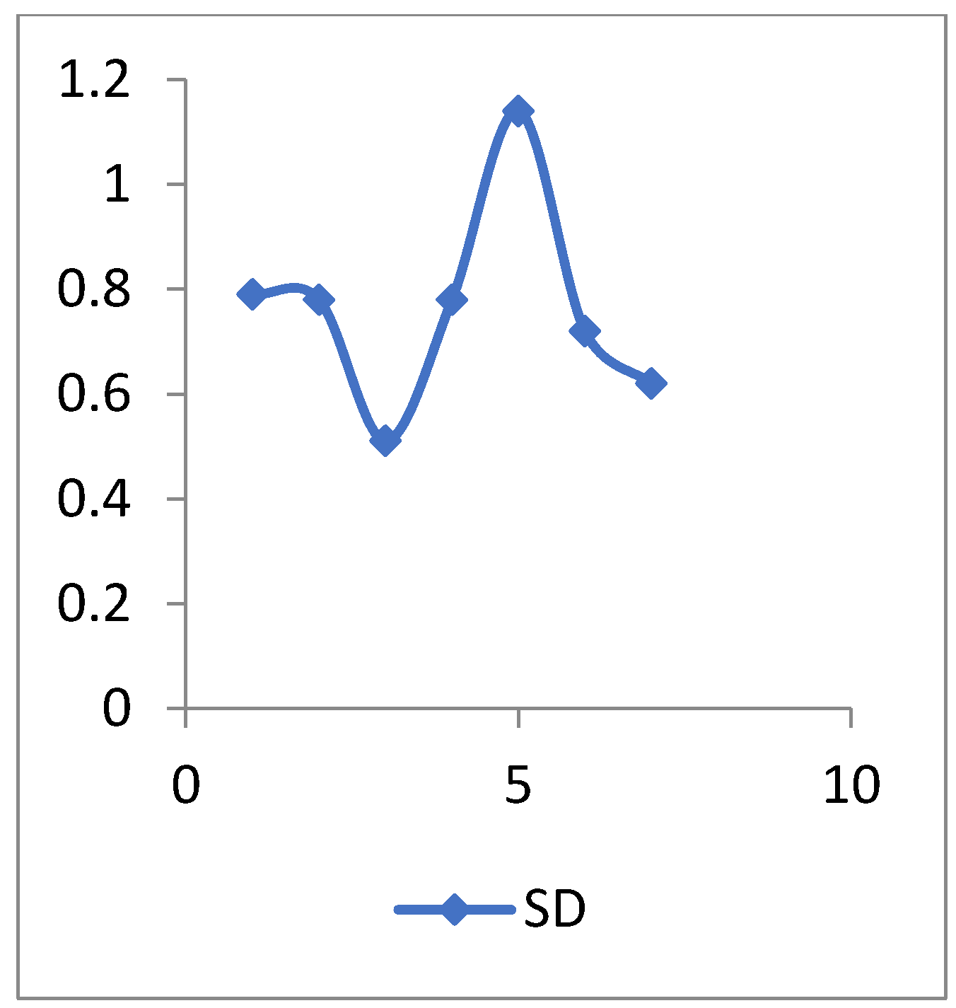
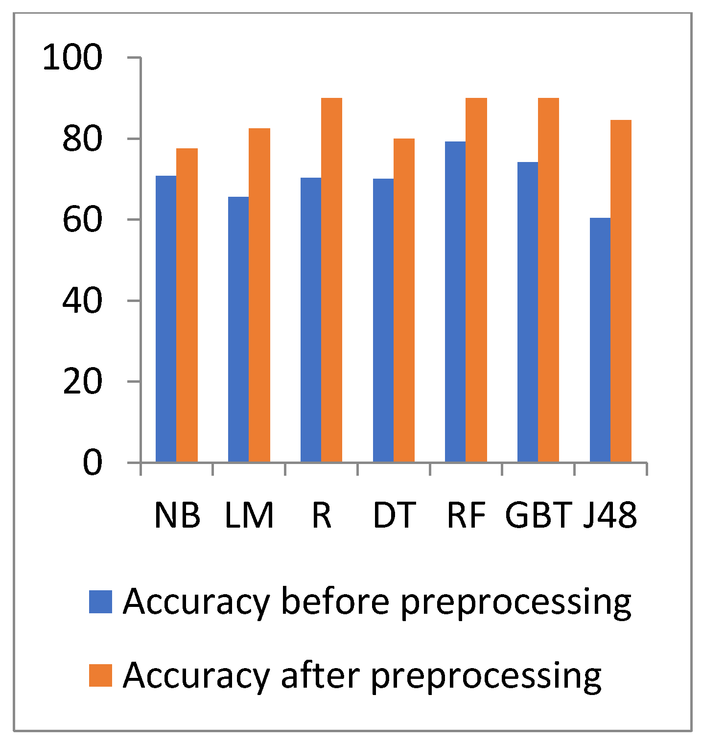
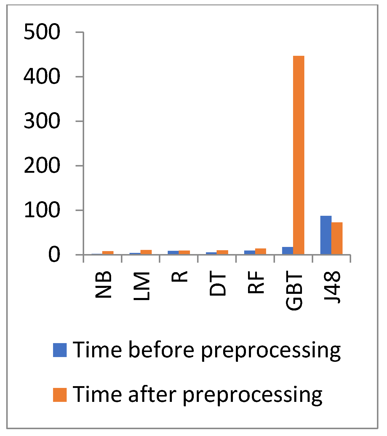
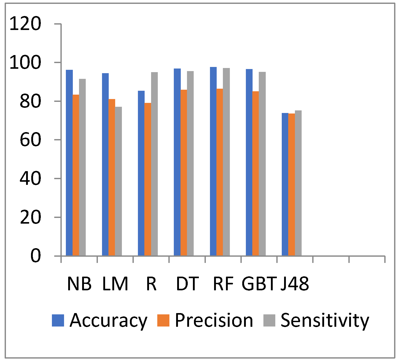
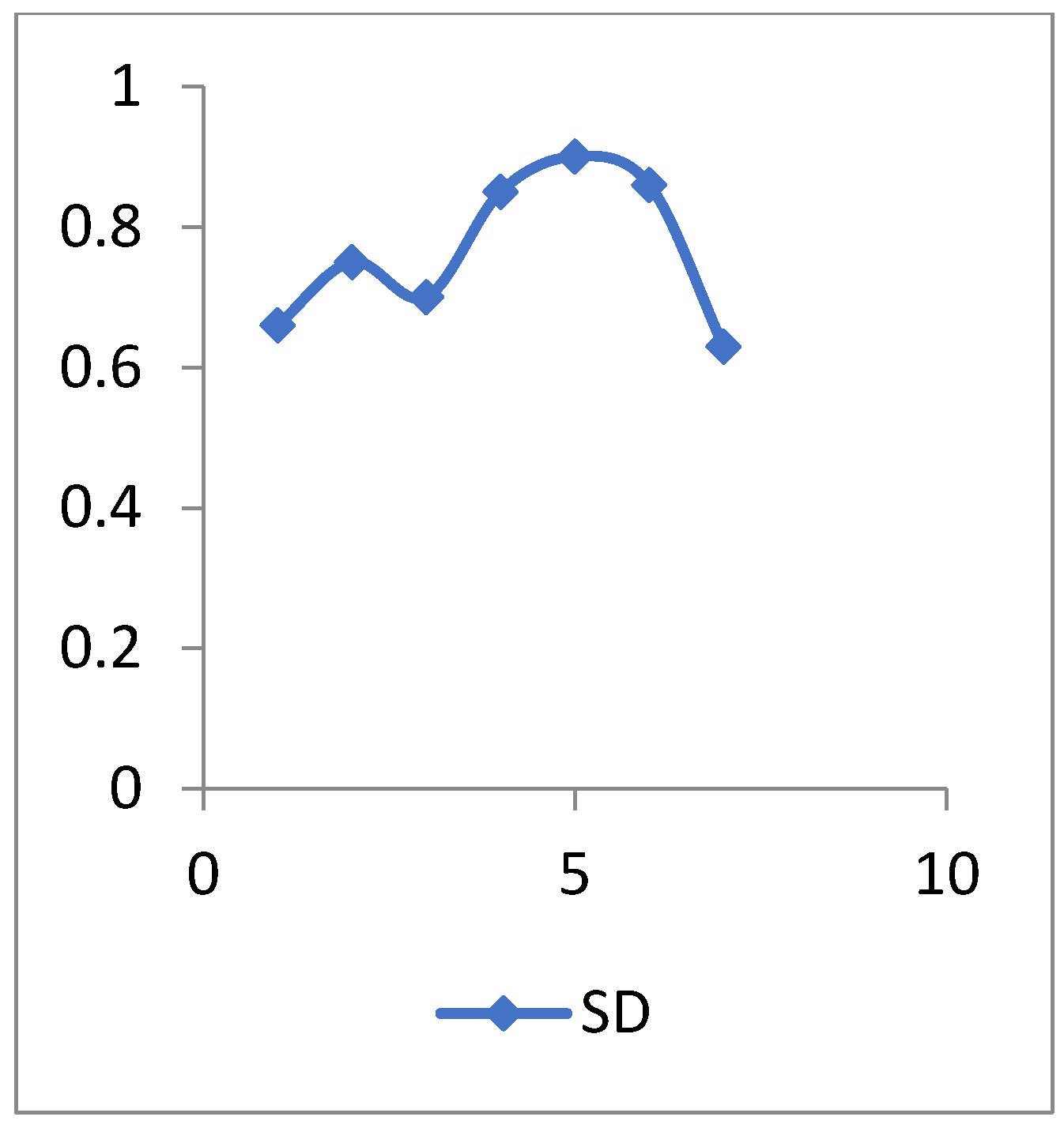
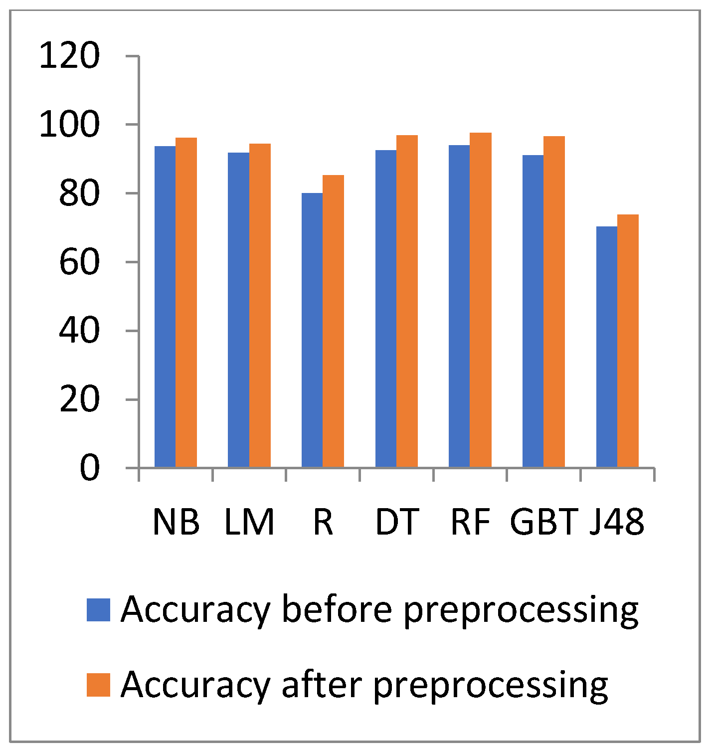
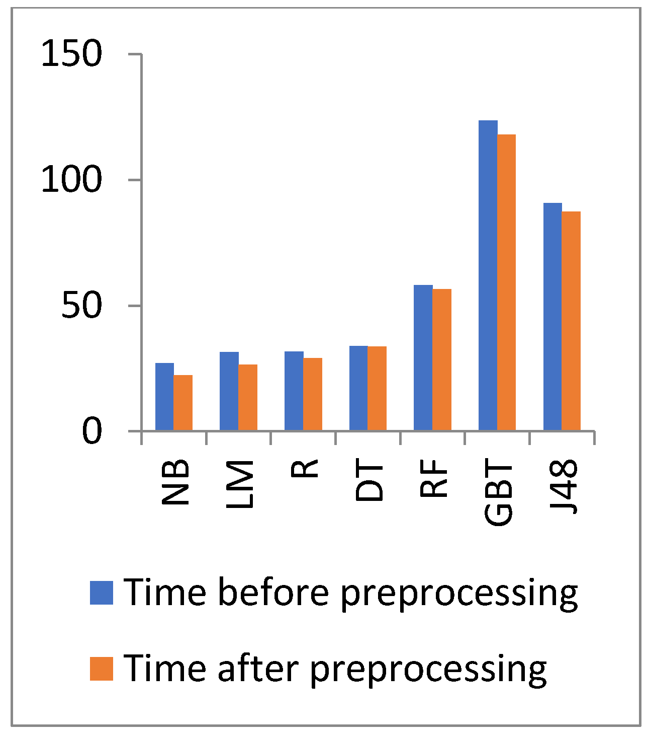
Figure 4 and Figure 5 show the representation of accuracy, precision, sensitivity, and standard deviation (SD) for the heart disease dataset. Figure 6 and Figure 7 show the comparison between the accuracy and time results of the data before and after preprocessing.

In Figure 6 and Figure 7, the results show that the accuracy after preprocessing is better than without preprocessing for all of the tested algorithms on the heart disease dataset. Moreover, for time processing, the time processing of the algorithms without a preprocessing is longer than the time processing of the preprocessed data.

Figure 8 and Figure 9 show the representation of accuracy, precision, sensitivity, and SD for the general health dataset. Figure 10 and Figure 11 show the comparison between the accuracy and time results of the data before and after preprocessing.

In Figure 10 and Figure 11, the results show that the accuracy after preprocessing is better than without preprocessing for all of the tested algorithms on the general health dataset. Moreover, for time processing, the time processing of the algorithms without preprocessing is longer than the time processing of the preprocessed data.

Figure 12 and Figure 13 show the representation of accuracy, precision, sensitivity, and SD for the diabetes dataset. Figure 14 and Figure 15 show the comparison between the accuracy and time results of the data before and after preprocessing.

The standard deviation (SD) is a descriptive statistic that measures the amount of variation or dispersion in a set of numbers. A low SD implies that the values are close to the mean of a set (also known as the expected value), whereas a high SD shows that the values are spread over a larger range.

In Figure 14 and Figure 15, the results show that the accuracy after preprocessing is better than without preprocessing for all of the tested algorithms on the diabetes dataset. Moreover, for time processing, the time processing of the algorithms without a preprocessing is longer than the time processing of preprocessed data.

The performance results are calculated using the following equations:

$$\mathbf{Precision}\mathbf{=}\frac{\mathbf{TP}}{\mathbf{TP}\mathbf{+}\mathbf{FP}}$$

(3)

$$\mathbf{Accuracy}\mathbf{=}\frac{\mathbf{TP}\mathbf{+}\mathbf{TN}}{\mathbf{TP}\mathbf{+}\mathbf{TN}\mathbf{+}\mathbf{FP}\mathbf{+}\mathbf{FN}}$$

(4)

$$\mathbf{Sensitivity}\mathbf{,}\mathbf{Recall}(\mathbf{TP}\mathbf{rate})\mathbf{=}\frac{\mathbf{TP}}{\mathbf{TP}\mathbf{+}\mathbf{FN}}$$

(5)

$$\mathbf{Relative}\mathbf{Error}\mathbf{=}\frac{\mathbf{Absolute} \mathbf{error} \mathbf{\ast } \mathbf{100}\mathbf{\%}}{\mathbf{“}\mathbf{True}\mathbf{”} \mathbf{value}}$$

(6)

where TP is the true positive value, TN is the true negative value, FP is the false positive value, and FN is the false negative value.

With regards to the diabetes dataset, the data have increased, and thus the processing time of the experimented algorithms increased. The highest accuracy is for the RF algorithm with a 97.58% value, but the lowest accuracy is 73.828% for the J48 algorithm. The J48 accuracy decreases when the data increase. The best time is 22.374 s for the NB algorithm, but the GBT has the highest processing time with 117.845 s.

From the results of the M-health and diabetes datasets, we conclude that the accuracy of J48 decreases as the data increase. Moreover, the GBT has the highest processing time when the data increase.

However, the NB processing time for the M-health and diabetes datasets is higher than the processing time of the heart disease dataset, but the NB remains as the algorithm with the least processing time.

5.3. Discussion

The experimental results show that the proposed model provides comparable results of different classification algorithms. We implemented these algorithms once without the use of the CFS reduction algorithm, and a second time after applying the CFS algorithm. The results show that the different classification algorithms with a combination of CFS provide significant values of accuracy. In contrast, the best accuracy value of the three datasets is provided by the RF with a combination of CFS. Here, we conclude that the accuracy of J48 decreases when the data increase. Moreover, the GBT has the highest processing time when the data increase.

The NB processing time for the three datasets is the highest, and thus the NB is the algorithm with the least processing time.

The main factors that lead to better accuracy results are as follows:

-

Preprocessing helps in increasing the data quality, since good data quality results in good accuracy values.

-

The application of data reduction algorithm reduces the consuming time.

-

The limitations or challenges of our model are as follows:

-

Time complexity: The execution requires a large amount of time, since the more the data increase, the more time it requires for the execution.

-

CPU processing issues, such as data with a high volume require a major part of the computer memory.

-

Adjusting the parameters’ values, such as the number of layers, max_depth, etc. requires significant effort and time since it is a trial-and-error experiment.

6. Conclusions

Medical big data are generated due to the vast increase of existing devices, sensors, actuators, and network communications. From a data mining perspective, the medical data classification steps include data acquisition, data preprocessing, feature extraction, and training-testing classification phases. In this paper, we first collected data from different resources, then cleaned them and filled in the missing data. Thereafter, we selected the features, which are useful for data reduction. Finally, we used seven different data classification algorithms, including NB, LM, R, DT, RF, GBT, and J48. After conducting our experiments, we conclude that the RF has the best classification accuracy with values of 97.58, 83.59, and 90% for heart disease, M-health, and diabetes datasets, respectively. However, the NB has the best running time with values of 0.078, 7.683, and 22.374 s for heart disease, M-health, and diabetes datasets, respectively. The results of applying RF with a combination of CFS on the heart disease dataset are as follows: Accuracy of 90%, precision of 83.3%, sensitivity of 100, and consuming time of 3 s. In addition, the results of applying this approach on the M-health dataset are as follows: Accuracy of 83.59%, precision of 74.3%, sensitivity of 93.1, and consuming time of 13.481 s. Moreover, the results on the diabetes dataset are as follows: Accuracy of 97.58%, precision of 86.39%, sensitivity of 97.14, and consuming time of 56.508 s. In the future, we will enhance the accuracy of the RF classification algorithm by implementing different reduction algorithms. Furthermore, we intend to implement a hybrid between RF and NB. Of note, although the RF gives the highest accuracy, it takes the longest processing time. In this case, the use of NB algorithm will solve this problem.

References

- Maleki, N.; Zeinali, Y.; Niaki, S. A k-NN method for lung cancer prognosis with the use of a genetic algorithm for feature selection. Expert Syst. Appl. 2021, 164, 113981. [Google Scholar] [CrossRef]
- Bichri, A.; Kamzon, M.; Abderafi, S. Artificial neural network to predict the performance of the phosphoric acid production. Procedia Comput. Sci. 2020, 177, 444–449. [Google Scholar] [CrossRef]
- Aurelia, J.; Rustam, Z.; Wirasati, I.; Hartini, S.; Saragih, G. Hepatitis classification using support vector machines and random forest. IAES Int. J. Artif. Intell. (IJ-AI) 2021, 10, 446–451. [Google Scholar] [CrossRef]
- Ehatisham-ul-Haq, M.; Malik, M.; Azam, M.; Naeem, U.; Khalid, A.; Ghazanfar, M. Identifying Users with Wearable Sensors based on Activity Patterns. Procedia Comput. Sci. 2020, 177, 8–15. [Google Scholar] [CrossRef]
- Ye, Y.; Shi, J.; Zhu, D.; Su, L.; Huang, J.; Huang, Y. Management of medical and health big data based on integrated learning-based health care system: A review and comparative analysis. Comput. Methods Programs Biomed. 2021, 209, 106293. [Google Scholar] [CrossRef] [PubMed]
- Nandhini, S.; JeenMarseline, K.S. Performance Evaluation of Machine Learning Algorithms for Email Spam Detection. In Proceedings of the International Conference on Emerging Trends in Information Technology and Engineering (ic-ETITE), Vellore, India, 24–25 February 2020; pp. 1–4. [Google Scholar]
- Nasiri, S.; Khosravani, M. Machine learning in predicting mechanical behavior of additively manufactured parts. J. Mater. Res. Technol. 2021, 14, 1137–1153. [Google Scholar] [CrossRef]
- Jalota, C.; Agrawal, R. Analysis of Educational Data Mining using Classification. In Proceedings of the International Conference on Machine Learning, Big Data, Cloud and Parallel Computing(Com-IT-Con), Faridabad, India, 14–16 February 2019; pp. 1–5. [Google Scholar]
- Rumsfeld, J.; Joynt, K.; Maddox, T. Big data analytics to improve cardiovascular care: Promise and challenges. Nat. Rev. Cardiol. 2016, 13, 350–359. [Google Scholar] [CrossRef]
- Lee, C.; Yoon, H. Medical big data: Promise and challenges. Kidney Res. Clin. Pract. 2017, 36, 3–11. [Google Scholar] [CrossRef] [PubMed] [Green Version]
- Costa, R.; Moreira, J.; Pintor, P.; dos Santos, V.; Lifschitz, S. A Survey on Data-driven Performance Tuning for Big Data Analytics Platforms. Big Data Res. 2021, 25, 100206. [Google Scholar] [CrossRef]
- Gavai, G.; Nabi, M.; Bobrow, D.; Shahraz, S. Heterogenous Knowledge Discovery from Medical Data Ontologies. In Proceedings of the IEEE International Conference on Healthcare Informatics, Park City, UT, USA, 23–26 August 2017; pp. 519–523. [Google Scholar]
- Ansari, M.F.; Alankar, B.; Email, H.K. A Prediction of Heart Disease Using Machine Learning Algorithms. In Proceedings of the International Conference on Image Processing and Capsule Networks, Bangkok, Thailand, 6–7 May 2020; pp. 497–504. [Google Scholar]
- Singh, J.; Bagga, S.; Kaur, R. Software-based Prediction of Liver Disease with Feature Selection and Classification Techniques. Procedia Comput. Sci. 2020, 167, 1970–1980. [Google Scholar] [CrossRef]
- Kondababu, A.; Siddhartha, V.; Kumar, B.; Penumutchi, B. A comparative study on machine learning based heart disease prediction. In Materials Today: Proceedings; Elsevier: Amsterdam, The Netherlands, 2021; Volume 10, pp. 1–5. [Google Scholar] [CrossRef]
- Ali, M.; Paul, B.; Ahmed, K.; Bui, F.; Quinn, J.; Moni, M. Heart disease prediction using supervised machine learning algorithms: Performance analysis and comparison. Comput. Biol. Med. 2021, 136, 104672. [Google Scholar] [CrossRef] [PubMed]
- Abdulhamit, S.; Mariam, R.; Rabea, K.; Kholoud, K. IOT Based Mobile Healthcare System for Human Activity Recognition. In Proceedings of the 15th Learning and Technology Conference (L&T), Jeddah, Saudi Arabia, 25–26 February 2018; pp. 29–34. [Google Scholar]
- Jan, M.; Awan, A.; Khalid, M.; Nisar, S. Ensemble approach for developing a smart heart disease prediction system using classification algorithms. Res. Rep. Clin. Cardiol. 2018, 9, 33–45. [Google Scholar] [CrossRef] [Green Version]
- Khan, N.; Husain, S.M.; Tripathi, M.M. Analytical Study of Big Data Classification. In Proceedings of the ACEIT Conference Proceeding, Garden City, Bengaluru, March 2016; pp. 143–146. [Google Scholar]
- Mercaldo, F.; Nardone, V.; Santone, A. Diabetes Mellitus Affected Patients Classification and Diagnosis through Machine Learning Techniques. Procedia Comput. Sci. 2017, 112, 2519–2528. [Google Scholar] [CrossRef]
- Arul Jothi, K.; Subburam, S.; Umadevi, V.; Hemavathy, K. Heart disease prediction system using machine learning. Mater. Today Proc. 2021, 12, 1–3. [Google Scholar] [CrossRef]
- Arumugam, K.; Naved, M.; Shinde, P.; Leiva-Chauca, O.; Huaman-Osorio, A.; Gonzales-Yanac, T. Multiple disease prediction using Machine learning algorithms. Mater. Today Proc. 2021, 7, 1–4. [Google Scholar] [CrossRef]
- Pinto, A.; Ferreira, D.; Neto, C.; Abelha, A.; Machado, J. Data Mining to Predict Early Stage Chronic Kidney Disease. Procedia Comput. Sci. 2020, 177, 562–567. [Google Scholar] [CrossRef]
- Mateo, J.; Rius-Peris, J.; Maraña-Pérez, A.; Valiente-Armero, A.; Torres, A. Extreme gradient boosting machine learning method for predicting medical treatment in patients with acute bronchiolitis. Biocybern. Biomed. Eng. 2021, 41, 792–801. [Google Scholar] [CrossRef]
- Sabeena, B.; Sivakumari, S.; Amudha, P. A technical survey on various machine learning approaches for Parkinson’s disease classification. Mater. Today Proc. 2020, 10, 1–5. [Google Scholar] [CrossRef]
- Analytics Vidhya. Available online: https://www.analyticsvidhya.com/blog/2021/05/25-questions-to-test-your-skills-on-decision-trees/ (accessed on 31 December 2021).
- Muhammad, L.J.; Islam, M.M.; Usman, S.S.; Ayon, S.I. Predictive Data Mining Models for Novel Coronavirus (COVID 19) Infected Patients’ Recovery. SN Comput. Sci. 2020, 1, 200–206. [Google Scholar] [CrossRef]
- Genuer, R.; Poggi, J.M. Random Forests. In Random Forest in R; H2O.ai Inc., Springer Nature: Cham, Switzerland, 2020; pp. 33–51. [Google Scholar] [CrossRef]
- Medium. Available online: https://medium.com/m/globalidentity?redirectUrl=https%3A%2F%2Ftowardsdatascience.com%2Frandom-forests-an-ensemble-of-decision-trees-37a003084c6c (accessed on 31 December 2021).
- Ihya, R.; Namir, A.; El Filali, S.; DAOUD, M.A.; Guerss, F. J48 algorithm of machine learning for predicting user’s the acceptance of an E-orientation systems. In Proceedings of the 4th International Conference, Casablanca, Morocco, 2 October 2019; pp. 1–9. [Google Scholar]
- Nykodym, T.; Tom Kraljevic, T.; Wang, A. Generalized Linear Modeling with H2O, 6th ed.; Bartz, A., Ed.; H2O.ai, Inc.: Mountain View, CA, USA, 2017; pp. 14–45. [Google Scholar]
- Boateng, E.Y.; Abaye, D.A.A. Review of the Logistic Regression Model with Emphasis on Medical Research. J. Data Anal. Inf. Processing 2019, 7, 190–207. [Google Scholar] [CrossRef] [Green Version]
- Saberian, M.; Delgado, P.; Raimond, Y. Gradient Boosted Decision Tree Neural Network. arXiv 2019, arXiv:1910.09340. [Google Scholar]
- Dai, Y.; Sun, H. The naive Bayes text classification algorithm based on rough set in the cloud platform. J. Chem. Pharm. Res. 2014, 6, 1636–1643. [Google Scholar]
- Zhang, Y.; Wang, S.; Yang, X.; Dong, Z.; Liu, G.; Phillips, P.; Yuan, T. Pathological brain detection in MRI scanning by wavelet packet Tsallis entropy and fuzzy support vector machine. SpringerPlus 2015, 4, 201–209. [Google Scholar] [CrossRef] [PubMed] [Green Version]
- Sudirman, I.D.; Nugraha, D.Y. Naive Bayes Classifier for Predicting the Factors that Influence Death Due to COVID-19 In China. J. Theor. Appl. Inf. Technol. 2020, 98, 1686–1696. [Google Scholar]
- CIS. Available online: https://www.cisin.com/coffee-break/enterprise/highlights-the-advantages-and-disadvantages-of-machine-learning.html (accessed on 31 December 2021).
- Qiu, P.; Niu, Z. TCIC_FS: Total correlation information coefficient-based feature selection method for high-dimensional data. Knowl.-Based Syst. 2021, 231, 107418. [Google Scholar] [CrossRef]
- Banos, O.; Garcia, R.; Terriza, A.H.J.; Damas, M.; Pomares, H.; Rojas, I.; Saez, A.; Villalonga, C. mHealthDroid: A novel framework for agile development of mobile health applications. In Proceedings of the 6th International Work-conference on Ambient Assisted Living an Active Ageing, Belfast, UK, 2–5 December 2014; pp. 91–98. [Google Scholar]
- Kaggle: Your Machine Learning and Data Science Community. Available online: https://www.kaggle.com/brandao/diabetes?select=diabetic_data.csv (accessed on 11 October 2021).
- Catalog.data.gov. Available online: https://catalog.data.gov/dataset/heart-disease-mortality-data-among-us-adults-35-by-state-territory-and-county-2016-2018 (accessed on 13 October 2021).
Figure 1.
Big data formats.
Figure 2.
Random forest prediction [29].
Figure 3.
The proposed medical data classification model.
Figure 4.
Accuracy, precision, and sensitivity comparison of different algorithms on heart disease preprocessed data.
Figure 5.
The SD values of heart disease data.
Figure 6.
Accuracy comparison of different algorithms on heart disease before and after preprocessing.
Figure 7.
Time comparison of different algorithms on heart disease before and after preprocessing.
Figure 8.
Accuracy, precision, and sensitivity comparison of different algorithms on general health preprocessed data.
Figure 9.
The SD values of general health data.
Figure 10.
Accuracy comparison of different algorithms on general heath before and after preprocessing.
Figure 11.
Time comparison of different algorithms on general health before and after preprocessing.
Figure 12.
Accuracy, precision, and sensitivity comparison of different algorithms on diabetes disease preprocessed data.
Figure 13.
The SD values of diabetes disease data.
Figure 14.
Accuracy comparison of different algorithms on diabetes disease before and after preprocessing.
Figure 15.