Article

A Novel Narrowband Active Noise Control System with Online Secondary Path Modeling Based on Factor Decomposition and Application in Open Space

Key Laboratory for Optoelectronic Technology and System of the Education Ministry of China, College of Optoelectronic Engineering, Chongqing University, Chongqing 400044, China
*
Author to whom correspondence should be addressed.
Submission received: 20 December 2021 / Revised: 14 January 2022 / Accepted: 14 January 2022 / Published: 17 January 2022
(This article belongs to the Special Issue Noise Pollution and Environmental Sustainability)

Abstract

:

Featured Application

According to the established theoretical model, this study deduces the convergence conditions of the system and obtains the step-size bound suitable for all stages of system operation. The simulation and experimental results show that the system has excellent stability and robustness under extreme conditions; it has a pronounced noise reduction effect for different noise signals and establishes a quiet space. These results have practical guiding significance for other follow-up work, such as variable step size and auxiliary noise power scheduling strategy, as well as the creation of quiet space.

Abstract

Due to the complexity of the coupling between the active noise control (ANC) controller and secondary path estimator, performance analysis of the system becomes particularly difficult. At present, the performance analysis of the system is often based on the fact that the secondary path tends to be stable, and the secondary path fitting error is minimal. However, in the early stage of system operation, or when the secondary path changes suddenly, the secondary path fitting error is significant, which easily causes divergence of the system control. It is still unable to guarantee the step-size bounds of convergence stability. Therefore, factor decomposition was used to analyze the mean weight behavior in this study. This strategy emphasizes the influence of secondary path modeling (SPM) error. The mean square behavior was evaluated using the energy conservation relationship. According to the established theoretical model, the convergence condition of the system was derived and the upper bound of step size suitable for all stages of system operation was obtained. The simulation and experimental results show that the ANC system is quite stable and robust under extreme conditions and has an obvious noise reduction effect in a specific range of open space, which can reach about 20 dB noise reduction.

1. Introduction

Noise control methods mainly include passive and active control strategies [1,2,3]. Passive noise control improves ambient acoustic performance by absorbing materials and changing the shape of the structure in conjunction with the environment [4]. These methods have an obvious effect on reducing the middle- and high-frequency noise in the environment. However, it has a poor effect at low frequencies. The active noise control (ANC) system uses an adaptive algorithm to control the secondary source to generate a reverse secondary sound wave, which is superimposed with the primary sound field to achieve the purpose of canceling noise [5]. Compared to passive noise control methods, active noise control has a more significant effect on low-frequency noise control and has been widely used in building environments [6]. In an ANC system, the system identification technology is typically used to estimate the secondary path [7,8]. To compensate for the influence of the secondary path model (SPM), as an improvement of the least mean square algorithm, the filtered-x least mean square (FxLMS) algorithm is the most popular adaptive algorithm [9,10]. In the FxLMS algorithm, the reference signal must be filtered using the secondary path response function, and then the control filter coefficients must be updated. Therefore, it is necessary to fit the secondary path. The fitting methods of the secondary path are divided into online and offline fittings. In practical use, the adjustment of the power amplifier gain, the change in environment, and the aging of devices will cause the change in secondary path response function. Therefore, it is necessary to perform online fitting on the secondary path, and the FxLMS algorithm can maintain stability when the relative error of the secondary path is ± 90 ° [11,12]. Eriksson et al. first proposed the use of auxiliary noise to perform online fitting on the secondary path [13]. This marked a new journey to pursue a more efficient ANC system. In recent years, different strategies have been used to improve the convergence speed and steady-state performance of secondary path online fitting [14,15,16,17,18,19,20].
In the process of secondary path modeling (SPM), due to the interaction between the fitting errors of SPM and ANC filters, the FxLMS algorithm is more complicated than the least mean square (LMS) system. More specifically, the accuracy of the ANC control filter fitting affects the accuracy of the error signal used to update the SPM filter. This situation is more complex for an ANC control filter. The accuracy of the SPM filter not only affects the accuracy of the error signal, but also affects the accuracy of the reference signal used to update the ANC filter.
Many researchers have conducted detailed analyses and discussions on important issues, such as convergence speed, steady-state mean square error, and system stability for ANC systems. Bjarnason analyzed the performance of FxLMS on the mean and mean square using a spherical invariant process. It was found that the delay in the coefficient update had only a minor effect on the stability bounds and steady-state behavior of a Gaussian white noise input [21]. Without using the independence assumption, Tobias et al. conducted a comprehensive analysis of the convergence performance of the FxLMS on the mean. Comprehensive research was conducted on the mean weight behavior of the FxLMS, and the impact of the error in SPM was studied [22]. Ardekani et al. analyzed the convergence of the ANC system with band-limited white noise and the moving average secondary path. In addition, the pure delay secondary path was discussed in detail. Through a linear model, the upper bound of the adaptive step length was derived [23].
Zhang et al. analyzed the influence of auxiliary noise power using the mean square criterion and determined the optimal step size of the ANC system [24]. Xiao et al. conducted a comprehensive theoretical analysis of the narrowband ANC system fitted online using the secondary path. For the narrowband ANC system, the difference equation determines the dynamic performance of the system and derives the closed expression of the system in the steady state [25]. Liu et al. proposed a strategy for scaling auxiliary noise based on the properties of the narrowband ANC system to improve its convergence and steady-state performance [26]. Chan et al. used Gaussian white noise as the input signal and found that the difference equation describes the convergence performance of the system in terms of the mean and mean square. In addition, the steady-state error was used to decouple the difference equations to obtain the stability conditions of the system, and an auxiliary noise adjustment method was proposed [9]. Miyoshi et al. used statistical mechanics methods to analyze the mean square error of the FxLMS in the steady and transient states. Under the actual primary path condition, the theoretical model above can analyze the input signal of non-Gaussian white noise [27,28]. Yang et al. used an enhanced weighted vector to analyze the performance of any input reference signal and derived its stability bound [10]. However, the calculation of the eigenvalues of the correlation matrix is complicated.
The above analysis of ANC filter convergence performance is based on the condition that the secondary path tends to be stable. In other words, the upper bound of the step size of the ANC filter can only be obtained if the relative error of the secondary path is small. To ensure the stability of the system, most online SPM methods have to use offline modeling for a period of time in advance so that the relative error of the secondary path is less than that of 5   dB [14,15,17,18]. This cannot guarantee the convergence of the system in the start-up stage, and sometimes the system does not have the conditions for offline modeling. Moreover, a sudden change in the secondary path can occur when the system is running. The change in the power amplification gain may cause a sizeable relative error in the secondary path and divergence of the entire system.
In this paper, to study the influence of secondary path error on the ANC system, especially in the start-up stage and the sudden change in the secondary path, we analyze the performance of the ANC system with online SPM in detail. First, the factor decomposition method was used to derive the mean convergence condition of the algorithm according to the properties of the secondary path error matrix. The error matrix combined with the characteristics of the secondary path determines the upper bound of the step size of the ANC filter, which changes with the operation of the SPM filter. Second, the energy conservation relation was used to analyze the mean square convergence. Finally, we derived the steady-state mean square error (MSE) of the ANC system. The simulation and experimental results show that the system is quite stable under extreme conditions and has a noticeable noise reduction effect in a specific range of open space, which provides a basis for the ANC system design.

2. The Whole Stage Stability of the ANC System with Online SPM

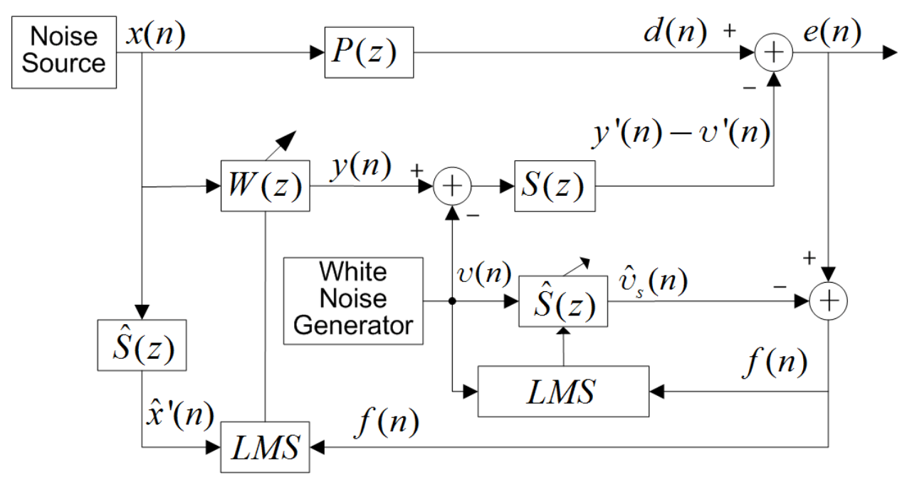
Figure 1 shows an online secondary modeling ANC system with auxiliary noise. From the results of previous studies [29], it can be observed that the update of the SPM filter is computed as:
s ^ ( n + 1 ) = s ^ ( n ) + μ s υ ( n ) f ( n ) ,
where s ^ ( n ) = [ s ^ 0 ( n ) s ^ 1 ( n ) s ^ M 1 ( n ) ] T is the coefficient vector of the SPM filter with length M and f ( n ) is the error signal used to update the SPM and ANC filters. υ ( n ) is a Gaussian white noise vector and μ s is the step-size factor of the SPM filter. Before using the reference signal x ( n ) to update the ANC filter, it must be filtered by the secondary path s ( n ) . If s ( n ) is unknown, s ( n ) is replaced by s ^ ( n ) . The ANC filter update equation is as follows:
w ( n + 1 ) = w ( n ) + μ w x ( n ) f ( n ) ,
where x ( n ) = [ x ( n ) x ( n 1 ) x ( n L + 1 ) ] T is the reference signal estimation vector with length L , w ( n ) is the coefficient vector of the ANC filter with length L , and μ w is the step-size factor of the ANC filter. Then, we will analyze the convergence performance of the ANC system, particularly the influence of the relative error of the secondary path on the system.
To simplify the analysis, we make the following assumptions:
  • The reference signal x ( n ) is white noise with a Gaussian distribution, the mean value is zero, and the variance is σ x 2 . Therefore, there is no correlation between the reference signal vectors x ( n ) , x ( n 1 ) , x ( n 2 ) , ;
  • The auxiliary noise υ ( n ) is Gaussian white noise with a zero mean and variance σ υ 2 . Moreover, υ ( n ) and x ( n ) are independent;
  • The coefficient vector w ( n ) and reference signal vector x ( n ) are independent, which is a widely used assumption.

2.1. Mean Weight Behavior

2.1.1. SPM Filter

The residual error f ( n ) contains three parts: error e x ( n ) caused by the ANC filter, error e υ ( n ) caused by the SPM filter, and background noise u ( n ) .
f ( n ) = e x ( n ) + e υ ( n ) + u ( n ) ,
where:
e x ( n ) = d ( n ) y ( n ) ,
e υ ( n ) = s T ( n ) υ L ( n ) s ^ T ( n ) υ M ( n ) .
Combining with assumptions 1–3, the variance of f ( n ) can be expressed as:
E ( f 2 ( n ) ) = E ( e x 2 ( n ) ) + E ( e υ 2 ( n ) ) + E ( u 2 ( n ) ) ,
where E [ ] denotes the expectation operator. The Wiener solution s of the secondary path can be obtained by substituting (5) into (6):
s = ( E ( υ M ( n ) υ M T ( n ) ) ) 1 E ( υ M ( n ) υ L T ( n ) ) s ( n ) .
It can be seen M L , s = s ( n ) . If M < L , a modeling error exists. In practical applications, s ( n ) is an FIR filter. Therefore, reducing or eliminating the modeling error is always possible by making M a larger value. In order to simplify the analysis and not lose generality, we set M = L in this paper. For the auxiliary noise vector υ T ( n ) , the subscript is no longer used to indicate the length.
Let the error coefficient vector of the SPM filter be Δ s ( n ) = s ^ ( n ) s ( n ) = [ Δ s L 1 ( n ) , Δ s L 2 ( n ) , , Δ s 0 ( n ) ] . Subtract s ( n ) from both sides of Equation (1) and take expectation:
E ( Δ s ( n + 1 ) ) = E ( Δ s ( n ) ) μ s E ( υ ( n ) ( e x ( n ) + e υ ( n ) + u ( n ) ) ) = ( I μ s E ( υ ( n ) υ T ( n ) ) ) E ( Δ s ( n ) ) ,
where I denotes an identity matrix with compatible dimensions. It can be seen from (8) that, to ensure convergence to the optimal solution, the condition μ s 2 / λ g , max must be met. λ g , max is the largest eigenvalue of the covariance matrix E ( υ ( n ) υ T ( n ) ) . Because υ ( n ) is Gaussian white noise, all eigenvalues of the correlation matrix are σ υ 2 . Therefore μ s must be less than 2 / σ υ 2 . σ υ 2 is also the power of the auxiliary noise. In addition, it can be observed that a larger auxiliary noise power can increase the convergence speed of the SPM filter, but it will reduce the steady-state performance of the ANC system. To balance the two conflicting requirements of fast convergence and low residual noise under steady-state conditions, several auxiliary noise power scheduling strategies have been proposed [15,18]. A larger auxiliary noise was used in the early stage of the system, and a smaller auxiliary noise was used when the system tended to converge.

2.1.2. ANC Filter

First, we show the Wiener solution of the ANC filter. The signal from the output y ( n ) of the ANC filter to the noise control point is:
y ( n ) = i = 0 L 1 s L 1 i y ( n i ) = i = 0 L 1 w T ( n i ) x ( n i ) s L 1 i = X s T ( n ) W ( n ) .
Combining (9) with (6):
E ( f 2 ( n ) ) = E ( e υ 2 ( n ) ) + E ( u 2 ( n ) ) + 2 i = 0 L 1 s L 1 i E ( d ( n ) x T ( n i ) ) w + w T j = 0 L 1 i = 0 L 1 s L 1 j s L 1 i E ( x ( n i ) x T ( n j ) ) w .
In (10), by taking the derivative of the vector w and setting the derivative to zero, the Wiener solution w of the ANC filter can be presented as:
w = R s s 1 P s ,
where:
R s s = j = 0 L 1 i = 0 L 1 s L 1 j s L 1 i E ( x ( n i ) x T ( n j ) ) = j = 0 L 1 i = 0 L 1 s L 1 j s L 1 i R j i ,
P s = i = 0 L 1 s L 1 i E ( d ( n ) x T ( n i ) ) .
The correlation matrix of the reference signal is defined as:
R i = E ( x ( n ) x T ( n i ) ) .
It is evident that R i = R i T .
Next, the steady-state solution of the ANC filter is derived. Combining Equations (2), (3) and (9), and taking the expectations on both sides of (2), we obtain:
E ( w ( n + 1 ) ) = E ( w ( n ) ) + μ w E ( X ( n ) s ^ ( n ) ( d ( n ) X s T ( n ) W ( n ) ) + e υ ( n ) + u ( n ) ) ) ,
where X ( n ) = [ x ( n ) , x ( n 1 ) , , x ( n + 1 L ) ] is the reference matrix. As n , E ( w ( n + 1 ) ) = E ( w ( n ) ) , we obtain:
E ( X ( n ) s ^ ( n ) X s T ( n ) ) W ( ) = E ( d ( n ) X ( n ) s ^ ( n ) ) ,
where W T ( ) = [ w T ( ) , w T ( ) , , w T ( ) ] T is the steady-state augmented weight vector. Using (16), the steady state can be derived as follows:
w ( ) = R s s ˜ 1 P s ˜ ,
where:
R s s ^ = j = 0 L 1 i = 0 L 1 s ^ L 1 j ( ) s L 1 i E ( x ( n i ) x T ( n j ) ) = j = 0 L 1 i = 0 L 1 s ^ L 1 j ( ) s L 1 i R j i ,
P s ^ = i = 0 L 1 s ^ L 1 i ( ) E ( d ( n ) x T ( n i ) ) .
As shown in (17), the accuracy of modeling the secondary path influences the steady state of the ANC filter. As in n , if the SPM filter converges to the actual secondary path, the ANC filter will converge to its Wiener solution.
We begin by analyzing the stability conditions of the ANC filter. The coefficient vector of the ANC filter is defined as Δ w ( n ) = w ( n ) w ( ) . The augmented coefficient vector of the ANC filter is:
Δ W ( n ) = W ( n ) W ( ) = Δ w ( n ) Δ w ( n 1 ) Δ w ( n + 1 L ) .
By using expressions (9) and (2), subtracting w ( ) from both sides of expression (2), Δ w ( n + 1 ) can be computed as:
Δ w ( n + 1 ) = Δ w ( n ) μ w G ( n ) Δ W ( n ) + μ w b ( n ) ,
where:
G ( n ) = [ G 0 ( n ) , G 1 ( n ) , , G L 1 ( n ) ] ,
G j ( n ) = ( i = 0 L 1 s L 1 i s L 1 j x ( n i ) ) x T ( n j ) + ( i = 0 L 1 Δ s L 1 i ( n ) s L 1 j x ( n i ) ) x T ( n j ) ,
b ( n ) = X ( n ) ( s ( n ) + Δ s ( n ) ) × ( d ( n ) s T X ( n ) w ( ) + u ( n ) + e υ ( n ) ) = X ( n ) ( s ( n ) + Δ s ( n ) ) ( η ( n ) + u ( n ) + e υ ( n ) ) ,
η ( n ) = d ( n ) s T X ( n ) w ( ) ,
where η ( n ) denotes the optimal error of the ANC filter. We assume that the update Δ w ( n ) is very slow and the value of μ w is so small that Δ w ( n ) Δ w ( n 1 ) Δ w ( n + 1 L ) , and we can obtain:
Δ w ( n + 1 ) = Δ w ( n ) μ w j = 0 L 1 G j ( n ) Δ w ( n ) + μ w b ( n ) = Δ w ( n ) μ w ( A ( n ) + B ( n ) ) Δ w ( n ) + μ w b ( n ) ,
where:
A ( n ) = j = 0 L 1 i = 0 L 1 ( s L 1 i s L 1 j x ( n i ) x T ( n j ) ) ,
Β ( n ) = j = 0 L 1 i = 0 L 1 ( Δ s L 1 i ( n ) s L 1 j x ( n i ) x T ( n j ) ) .
Taking expectations on both sides of (26) and using assumptions 1–3:
E ( Δ w ( n + 1 ) ) = E ( Δ w ( n ) ) + μ w E ( b ( n ) ) μ w E ( A ( n ) + B ( n ) ) E ( Δ w ( n ) ) .
Combining (16) and (24), and assumptions 1–3, one obtains:
E ( b ( n ) ) = 0 .
Substituting (30) into (29) yields:
E ( Δ w ( n + 1 ) ) = ( I μ w ( E ( A ( n ) ) + E ( B ( n ) ) ) ) E ( Δ w ( n ) ) .
Equation (31) suggests that the convergence of E ( Δ w ( n ) ) is determined by the eigenvalues of E ( A ( n ) ) + E ( B ( n ) ) . However, in the start-up stage of ANC system operation or a sudden change occuring in the secondary path, the value of Δ s ( n ) is large and unknown. Therefore, the eigenvalue of E ( A ( n ) ) + E ( B ( n ) ) is challenging to estimate. The relation is:
ρ ( E ( A ( n ) ) + E ( B ( n ) ) ) ρ ( E ( A ( n ) ) + ρ ( E ( B ( n ) ) ,
where ρ ( · ) represents the spectral radius of matrix. The upper bound of ρ ( E ( A ( n ) ) + E ( B ( n ) ) ) can be estimated using ρ ( E ( A ( n ) ) and ρ ( E ( B ( n ) ) . For convenience, the rows and columns of the matrices E ( A ( n ) ) and E ( B ( n ) ) start at zero. Because x ( n ) is white noise with Gaussian distribution, the ( k , m ) -element ( 0 m k N 1 ) of the matrices E ( A ( n ) ) and E ( B ( n ) ) can be simplified to:
a k m = σ x 2 j i = m k L 1 s L 1 i s L 1 j ,
b k m = σ x 2 j i = m k L 1 Δ s L 1 i s L 1 j .
Applying mean inequality, for any ( k , m ) , one can obtain:
a k m σ x 2 i j = k m L 1 s L 1 i 2 + s L 1 j 2 2 σ x 2 i = 0 L 1 s L 1 i 2 ,
b k m σ x 2 i j = k m L 1 Δ s L 1 i 2 + s L 1 j 2 2 σ x 2 i = 0 L 1 ( Δ s L 1 i 2 2 + s L 1 i 2 2 ) .
Using the relationship between the spectral radius and norm of the matrix, the upper bound of ρ ( E ( A ( n ) ) and ρ ( E ( B ( n ) ) can be estimated as:
ρ ( E ( A ( n ) ) E ( A ( n ) ) N σ x 2 i = 0 L 1 s L 1 i 2 ,
ρ ( E ( B ( n ) ) E ( B ( n ) ) N σ x 2 ( i = 0 L 1 ( Δ s L 1 i 2 2 + s L 1 i 2 2 ) .
Q represents the -norm of matrix Q . The -norm represents the maximum value of the sum of the absolute values of the rows. Combining (32), (37), and (38), we can obtain the upper bound of the μ w :
μ w 2 N ( i = 0 L 1 ( Δ s L 1 i 2 + 3 s L 1 i 2 ) σ x 2 .
The sum i = 0 L 1 Δ s L 1 i 2 can be estimated by (5) and (6).
E ( e υ 2 ( n ) ) = σ υ 2 i = 0 L 1 Δ s L 1 i 2 E ( f 2 ( n ) ) = E ( e υ 2 ( n ) + e x 2 ( n ) + u 2 ( n ) ) .
Let P f ( n ) = E ( f 2 ( n ) ) and P x ( n ) = E ( x 2 ( n ) ) represent the power of the error signal f ( n ) and reference signal x ( n ) , respectively. P f ( n ) and P x ( n ) are estimated using an exponentially smoothed estimator.
P f ( n + 1 ) = λ P f ( n ) + ( 1 λ ) f 2 ( n ) ,
P x ( n + 1 ) = λ P x ( n ) + ( 1 λ ) x 2 ( n ) ,
where λ is a forgetting factor close to one. Because the specific value of each s i is not known, it seems difficult to estimate i = 0 L 1 s L 1 i 2 . However, the sum shows the power amplification ability of the system to a certain extent. Here, it is assumed that the upper bound R of the signal power amplification gain is known. Even if the value of R is unknown, the measurement of K is relatively easy.
i = 0 L 1 s L 1 i 2 R .
Using (39)–(43), the upper bound of μ w can be expressed as:
μ w 2 N P x ( n ) ( P f ( n ) / σ υ 2 + 3 R ) .
This suggests that the stability condition changed with the relative error of the SPM filter. As the ANC and SPM filters converge, P f ( n ) / σ υ 2 3 R , the stability condition can be replaced by:
μ w 2 3 N R P x ( n ) ,
which is the stability condition for the mean square behavior in [9]. This is only acceptable when the relative error of the secondary path is small. The stability condition in Equation (44) is more robust. The upper bound given above is applicable to all periods of ANC system operation.

2.2. Mean Square Behavior

2.2.1. SPM Filter

The covariance matrix of υ ( n ) is defined as R υ υ ( n ) = E ( υ ( n ) υ T ( n ) ) . Multiplying Δ s ( n + 1 ) by its transpose and taking the expectation on both sides of its updating equation, the covariance matrix of Δ s ( n + 1 ) can be expressed as:
c s ( n + 1 ) = E ( Δ s ( n + 1 ) Δ s T ( n + 1 ) ) = c s ( n ) μ s c s ( n ) R υ υ ( n ) μ s R υ υ ( n ) c s ( n ) + μ s 2 E ( υ ( n ) υ T ( n ) c s ( n ) υ ( n ) υ T ( n ) ) + μ s 2 E ( υ ( n ) υ T ( n ) ( e x 2 ( n ) + u 2 ( n ) ) ,
For the fourth term, by applying the method introduced in [30], it can be simplified as:
E ( υ ( n ) υ T ( n ) c s ( n ) υ ( n ) υ T ( n ) ) = 2 R υ υ ( n ) c s ( n ) R υ υ ( n ) + R υ υ ( n ) t r ( R υ υ ( n ) c s ( n ) ) ,
where t r ( · ) is the trace of the matrix. Because υ ( n ) is Gaussian white noise, substituting (54) into (53) yields:
c s ( n + 1 ) = c s ( n ) 2 μ s σ υ 2 c s ( n ) + μ s 2 σ υ 4 ( 2 c s ( n ) + t r ( c s ( n ) I ) + μ s 2 σ υ 2 ( E ( e x 2 ( n ) ) + σ u 2 ) I ,
where I denotes an identity matrix with compatible dimension. It can be observed from the fourth term in (55) that the error of the ANC filter generates a driving term for the differential equation of the secondary path. However, we assumed that the excitation caused by the fifth term is finite. It can be treated as an LMS algorithm for stability analysis from the literature [9], and the stability condition can be obtained as:
μ s 2 3 t r ( R υ υ ( n ) ) = 2 3 L σ υ 2 .

2.2.2. ANC Filter

Multiplying Δ w ( n + 1 ) by its transpose and taking the expectation on both sides of its updating equation, the covariance matrix of Δ w ( n + 1 ) can be expressed as:
c w ( n + 1 ) = E ( Δ w ( n + 1 ) Δ w T ( n + 1 ) ) = c w ( n ) μ w E ( A ( n ) + B ( n ) ) ) c w ( n ) μ w c w ( n ) E ( A ( n ) + B ( n ) ) + μ w 2 E ( ( A ( n ) + B ( n ) ) c w ( n ) ( A ( n ) + B T ( n ) ) ) + μ w 2 E ( b ( n ) b T ( n ) ) .
However, the analysis of c w ( n ) is mathematically difficult because of the influence of the secondary path error. It can be seen from the properties of the elements that the convergence performance of c w ( n ) is dominated by t r ( cov ( Δ w ( n ) ) ) = q w ( n ) . Therefore, it can be transformed into studying the properties of q w ( n ) , which is also a method used in the literature [24]. q w ( n ) can be computed as:
q w ( n ) = E ( Δ w T ( n ) Δ w ( n ) ) .
Using (26) and (30) yields:
q w ( n + 1 ) = q w ( n ) 2 μ w E ( Δ w T ( n ) ( A ( n ) + B ( n ) ) T Δ w ( n ) ) + μ w 2 E ( Δ w T ( n ) ( A ( n ) + B ( n ) ) T × ( A ( n ) + B ( n ) ) Δ w ( n ) ) + μ w 2 E ( b T ( n ) b ( n ) ) .
As shown in the Appendix A, the second and the third term meet the inequalities:
E ( Δ w T ( n ) ( A ( n ) + B ( n ) ) T Δ w ( n ) ) N ( P f ( n ) / σ υ 2 + 3 R ) σ x 2 q w ( n ) ,
E ( Δ w T ( n ) ( A ( n ) + B ( n ) ) T ( A ( n ) + B ( n ) ) Δ w ( n ) ) 6 N 4 σ x 4 R ( R + P f ( n ) / σ υ 2 ) q w ( n ) .
From (53) and (54), the system is stable in the mean-square sense when the driving term is finite and the step size μ w satisfies:
μ w ( P f ( n ) / σ υ 2 + 3 R ) 3 N 3 σ x 2 R ( R + P f ( n ) / σ υ 2 ) 1 N 3 P x ( n ) ( 3 R + P f ( n ) / σ υ 2 ) .
In the derivation process, the convergence condition is significantly strengthened. Therefore, to improve the convergence speed in practical applications, the upper bound given in (55) can be increased appropriately.

2.2.3. Steady-State MSE

From (4) and e ( n ) = d ( n ) y ( n ) + υ ( n ) + u ( n ) , the steady-state MSE is given by:
E ( e 2 ( ) ) = E ( e x 2 ( ) ) + σ υ 2 s T s + σ u 2 ,
where:
E ( e x 2 ( ) ) = σ η 2 + t r ( E ( A ( ) c w ( ) ) ) ,
σ η 2 is the variance of η ( n ) . The second term on the right side of (57) is the steady-state excess MSE (EMSE) of the ANC filter. Using (50) the steady-state EMSE of the ANC filter can be expressed as:
t r ( E ( A ( ) c w ( ) ) ) = μ w 2 t r ( E ( A ( ) c w ( ) A ( ) ) + E ( B ( ) c w ( ) B T ( ) ) + μ w 2 t r ( E ( b T ( ) b ( ) ) ) .
Similar to n , Δ s ( n ) tends to a zero vector, which results in E ( B ( ) c w ( ) B T ( ) ) being small compared to E ( A ( ) c w ( ) A ( ) . Hence, E ( B ( ) c w ( ) B T ( ) can be neglected. Substituting (24) into (58) yields:
E ( b T ( ) b ( ) ) = ( σ η 2 + σ u 2 + σ e υ 2 ( ) ) ( E ( A ( ) ) + E ( C ( ) ) ) ,
where:
σ e υ 2 ( ) = t r ( E ( ( R υ υ c s ( ) ) ) ,
is the steady-state EMSE of SPM filter. The definition of C ( n ) is:
C ( n ) = j = 0 L 1 i = 0 L 1 ( Δ s L 1 i ( n ) Δ s L 1 j ( n ) x ( n i ) x T ( n j ) ) .
Using assumption 1, it can be derived that:
E ( C ( ) ) ) = σ x 2 E ( i = 0 L 1 Δ s L 1 i 2 ( ) ) = σ x 2 σ e υ 2 ( ) σ υ 2 I .
From (58), (59), and (62), the steady-state EMSE of ANC can be expressed as:
t r ( E ( A ( ) c w ( ) ) ) = μ w 2 t r ( E ( A ( ) c w ( ) A ( ) ) + μ w 2 ( σ η 2 + σ u 2 + σ e υ 2 ( ) ) σ x 2 σ e υ 2 ( ) σ υ 2 × t r ( E ( A ( ) ) + I ) .
Using (46), the steady-state EMSE of the SPM filter can be computed as:
σ e υ 2 ( ) = μ s L σ υ 2 ( σ e x 2 ( ) + σ u 2 ) ( 2 μ s σ υ 2 ( L + 2 ) ) .
As shown above, we cannot find the closed form of the steady-state EMSE of the ANC filter for the existence of E ( A ( ) c w ( ) A ( ) . Moreover, the SPM and the ANC filters’ steady-state EMSE are coupled with each other. Both steady-state EMSEs can be controlled by step size μ w and μ s . Therefore, when both filters tend to be stable, a smaller step-size factor can be used to reduce the excess mean square error of the system.

3. Simulation Results

In this section, the proposed algorithm for improving the stability of an ANC system is discussed. In most studies, offline SPM was performed before running the ANC filter. In this study, we ran the SPM and ANC filters simultaneously. This implies that the secondary path has a large relative error in the initial stage of the operation. The performance of the ANC system is evaluated based on the relative error of the secondary path, which is defined as follows:
Δ s ( n ) ( d B ) = 10 log 10 ( s ( n ) s ˜ ( n ) 2 s ( n ) 2 ) ,
Δ w ( n ) ( d B ) = 10 log 10 ( w o ( n ) w ( n ) 2 w ( n ) 2 ) ,
where w o ( n ) is the coefficient vector of the ANC filter obtained from the standard FxLMS algorithm and the coefficient vector of the secondary path filter is the real secondary path.
The structure of the ANC system was the same as that shown in Figure 1. The primary path was set as an FIR filter with a memory length of 48. The data for the primary path are from [31]. The order of the ANC filter is set to 64. Two types of reference signal were used. The first was white Gaussian noise with a zero mean and a variance of 1. The second factor is color noise. The colored noise is generated by a first-order AR process x ( n + 1 ) = 0.9 x ( n ) + β ( n ) , where β ( n ) is a Gaussian white noise with a mean value of 0. The variance of the color noise was normalized as 1. The variance of background noise was σ u 2 = 0.04 . The auxiliary noise was Gaussian white noise with a mean value of 0 and variance of σ υ 2 = 0.2 . The results were averaged over 100 independent trials.

3.1. Case I

In this experiment, the stability of the system will be studied in the presence of a strong variation in the primary and secondary paths. At stage I, in the first 50,000 simulation samples, the impulse response of the primary path and the secondary path is p 1 ( n ) , s 1 ( n ) , respectively. At stage II, from n = 50,000 to n = 100,000, the impulse response of the primary path and the secondary path is p 2 ( n ) , s 2 ( n ) , respectively. The impulse response of the primary path and secondary path is shown in Figure 2. p 1 ( n ) and s 1 ( n ) are set as:
p 1 ( n ) = [ p 1 ( 0 ) , p 1 ( 1 ) , , p 1 ( L p ) ] T ,
s 1 ( n ) = [ s 1 ( 0 ) , s 1 ( 1 ) , , s 1 ( L ) ] T ,
where L p = 48 is the order of primary path impulse response. p 2 ( n ) and s 2 ( n ) are set as:
p 2 ( n ) = [ p 1 ( 0 ) , 1 3 p 1 ( 0 ) p 1 ( 1 ) , , 1 3 p 1 ( L p 1 ) p 1 ( L p ) ] T ,
s 2 ( n ) = [ s 1 ( 0 ) , 1 3 s 1 ( 0 ) s 1 ( 1 ) , , 1 3 s 1 ( L s 1 ) s 1 ( L ) ] T .
According to the definition of μ w max in (44), μ w is set to μ w max / K , where K = 3 , 6 , 10 and μ s = 0.002 . P x ( 0 ) and P f ( 0 ) are initialized as 1, λ = 0.99 . The upper bound of R is set to 1. The simulation results are shown in Figure 3.
The system can remain stable with two different input signals. As can be seen from Figure 3a,c,d,f, the larger the μ w , the faster the ANC filter converges, but the steady-state relative error is also larger. Second, the system can remain stable when there is a sudden change in the secondary and the primary paths. The smaller the value of μ w , the smaller the fluctuation of the ANC filter. It seems surprising that the smaller step size has a faster convergence speed in stage II. When the relative error of the ANC filter reaches a minimum, there is a rising stage. This can be explained by Figure 3c,f. As the system converges, the value of μ w max gradually increases, which causes the steady-state relative error of the ANC filter to increase.
It can be seen from Figure 3b,e that the convergence speed and steady-state error of the SPM filter are almost the same in the three cases because of the same value of μ s . Figure 3b,c shows that μ w is controlled by the modeling accuracy of the secondary path. The value of μ w max was smaller at the initial stage of the system and when the secondary path underwent a sudden change. As the SPM filter converges, the value of μ w max gradually increases and tends to be stable. Figure 3d suggests that K = 3 results in a more significant steady-state relative error of ANC filter, which leads to a larger steady-state relative error for the SPM filter.

3.2. Case II

In this experiment, the stability of the system was studied using an auxiliary noise power scheduling strategy. Except for the variable power of the auxiliary noise, the other conditions were the same as those in Case I. The auxiliary noise is υ ( n ) = G ( n ) υ ( n ) , where:
G ( n ) = 2 P f ( n ) P e ( n ) ,
P e ( n ) , P f ( n ) is the power of e ( n ) , f ( n ) , respectively. The calculation of P e ( n ) can use the type of expression (41) and P e ( 0 ) is initialized to 1. The simulation results are presented in Figure 4.
For variable power auxiliary noise, the system remains stable. Figure 4a,b shows that the convergence speeds of the ANC and SPM filters were faster than those of Case I in stages I and II. It can be seen from Figure 4b,e that the time required for the SPM filter to reach a steady state is the same as in Case I, whereas the relative error of the SPM filter decreases to −10dB faster. Figure 4c,f suggests that the upper bound of the step size is larger than the upper bound in Case I at the beginning of stages I and II.

3.3. Case III

This experiment studied the stability of the system when the order of the SPM filter was insufficient. The order of the actual secondary path was set to 64 and the order of the SPM filter was set to 32. The other conditions were the same as those in Case 1. The simulation results are shown in Figure 5.
It can be seen from Figure 5a,c that, when the secondary path order is insufficient, the ANC filter converges, but the relative error in the steady state is larger. The convergence speed is the same as that in Case I. Figure 5b shows that, compared with the normal order, the secondary path undergoes a sudden change when the order is insufficient, and the upper bound is more diminutive. This is because the error caused by the secondary path fitting is more significant. However, the ANC system can still converge in a stable manner.

4. Experimental Results

To verify the noise reduction performance of the control system, noise control was performed on two different types of noise signals: a narrowband noise signal and a noise signal whose energy is concentrated in a specific band. In this study, TMS320C6748 of TI Company was used as the DSP control platform. The signal sampling rate was 8 kHz and the data width is 16 bit. In addition, this study detects the sound field distribution characteristics before and after noise reduction to verify the noise reduction performance of the system in an open space.

4.1. Noise Reduction Performance

Narrowband noise is noise whose energy is mainly concentrated at a specific frequency or at several specific frequencies. This noise is common in periodic noise sources, such as engine noise. We selected single-frequency, multi-harmonic-frequency, and fixed-frequency band noise for the experiments. The mean value of the white noise signal used in the experiment was 0 and the variance was 1000. The order of the secondary path filter is 128. The value of K is 6.
As shown in Figure 6, with an increase in ANC filter order, the noise reduction effect of the system was better. The increase in filter order will obviously challenge the computing resources of the system. When the bandwidth of the reference noise signal is small, the computational pressure on the control system can be reduced by reducing the order of the ANC filter. Due to the influence of the electric heating noise of the ANC system and irrelevant background noise in the environment, residual noise remained at the noise control point when the system was stable. The higher the orders of the ANC filter, the faster the convergence speed of the system. From Figure 6d, we can see that, if the order continues to increase, the improvement in the convergence speed of the system is not obvious. When the order of the ANC filter was 20, the ANC system also achieved a good noise reduction effect under the guarantee of convergence speed. Therefore, a relatively small ANC filter order can obtain a significant noise reduction effect when dealing with noise with a relatively single-frequency component.
As shown in Figure 7, noise control was performed on noise with multi-harmonic-frequency components. The multi-harmonic noise components were 200 Hz, 400 Hz, 600 Hz, and 800 Hz. Different orders were used to deal with the multi-harmonic noise. As the noise signal became complex, higher requirements were proposed for the order of the ANC filter. In the noise reduction in single-frequency noise, when the order of the ANC filter was 10, a noise reduction of more than 10 dB was achieved. However, for noise with multi-harmonic frequency, when the order of the ANC filter increased to 30, the residual error signal at the error microphone was greatly reduced, the overall noise reduction in the system reached 30 dB, and the convergence speed was obviously accelerated. Increasing the order of the ANC filter cannot further improve the convergence speed and the steady-state error of the system. Therefore, considering the hardware resources and selecting the appropriate order, the system can achieve a significant noise reduction effect. The noise reduction effect at 200 Hz was better than that at 800 Hz. This also showed that the noise reduction effect of the system decreased with the increase in noise frequency.
In practical applications, noise energy is concentrated in a specific frequency band. Therefore, it is necessary to verify the noise reduction effect of the system on narrowband noise. The noise band selected was 200–600 Hz, and the order of the ANC filter was 10, 25, and 40. As shown in Figure 8, it can be seen that narrowband noise presents a different noise reduction effect from that of multi-harmonic noise. First, for narrowband noise, the overall noise reduction effect of the system was less than that of multi-harmonic noise, and the maximum noise reduction was approximately 15 dB. This is because the frequency component of the narrowband noise is more complex. Second, the increase in the order of the ANC filter can still reduce the steady-state error of the system. However, the increase in order was different from that in the case of multi-harmonic noise and did not improve the convergence speed. With the increase in order, there were large fluctuations for different frequencies in the noise frequency band. It can be seen from the figure that the power spectral density after noise reduction was relatively uniform and the noise reduction effect on the low-frequency part was much better.

4.2. Noise Reduction Sound Field Distribution

We further analyzed the sound field distribution characteristics before and after noise reduction in the current ANC control system. To accurately and finely describe the sound pressure distribution in space (the granularity of the sound pressure measurement interval was very small), we selected a specific local space to measure the sound pressure, and the measurement granularity of the sound pressure was 2 cm. The sound pressure distribution was measured within a certain spatial range. We used a plate with a length scale label to determine the relative position of the microphone in space. The scale on the plate was in centimeters. The plate was removed when its position was fixed. The noise source adopted a noise signal of 200–600 Hz, and the space size of the sound field was 30 cm × 15 cm. The sound pressure distribution before and after noise reduction was measured 768 times. The positions of the experimental layout position are shown in Figure 9.
As shown in Figure 10, the sound field distribution of the selected spatial range before and after noise reduction and the noise reduction amount of the corresponding points were shown. As shown in Figure 10a, there was a maximum sound pressure near the noise source of approximately 91 dB. The sound pressure gradually attenuated with increasing distance from the noise source. The sound pressure was relatively evenly distributed within the range of 0 cm to 10 cm length, 0 cm to 15 cm width, and 0 cm to 5 cm altitude. The sound pressure changed more slowly with an increase in the distance between the measuring point and the noise source. As can be seen from the distribution of the sound pressure after noise reduction in Figure 10b,c, the noise pressure was enhanced near the secondary sound source, and the sound pressure in the space near the noise control point had an obvious noise reduction effect, with a maximum noise reduction amount of about 20 dB. The noise reduction of approximately 15 dB was achieved at 0–4 cm length, 10–15 cm width, and 0–5 cm altitude. A noise reduction of approximately 20 dB was achieved near the error microphone. In the spatial range of 0–4cm length, 10–15 cm width, and 0–5cm altitude, noise reduction up to 15 dB was realized. Figure 10d shows the distribution of the mean value of the noise reduction at different altitudes in the length–width plane in Figure 10c. The overall mean distribution of the noise reduction in the length–width plane is displayed more intuitively. It can be seen from the figure that the ANC system adopted in this study had an obvious noise reduction effect in the space where the control point was located, except near the noise source and secondary sound source.

5. Conclusions

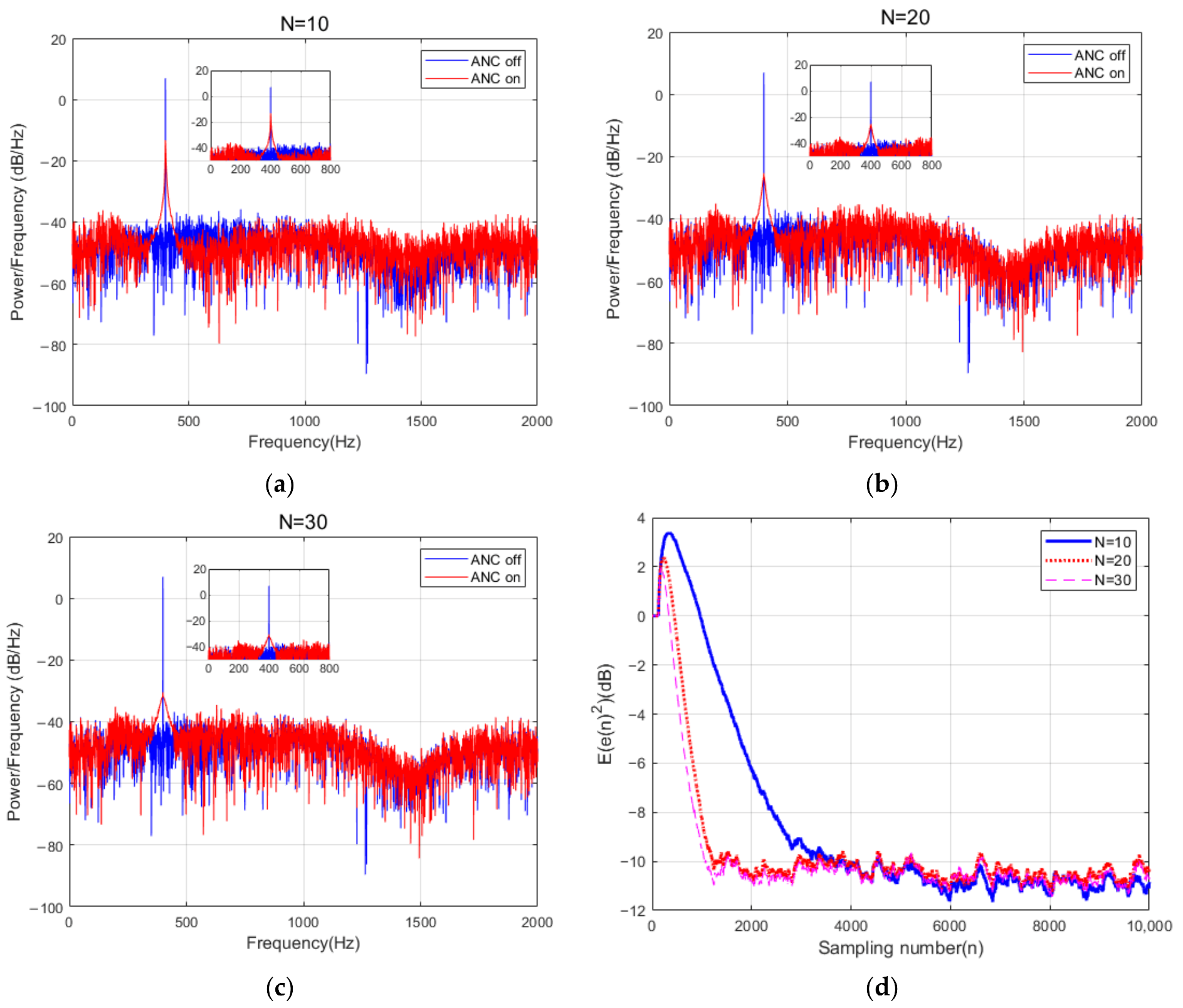
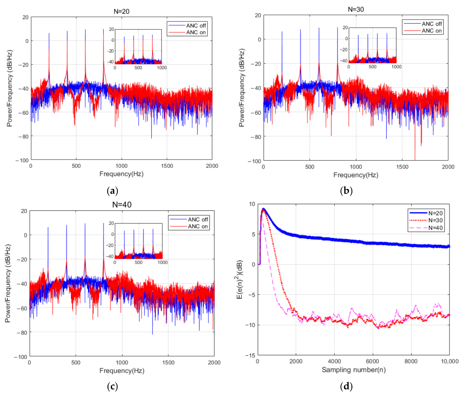
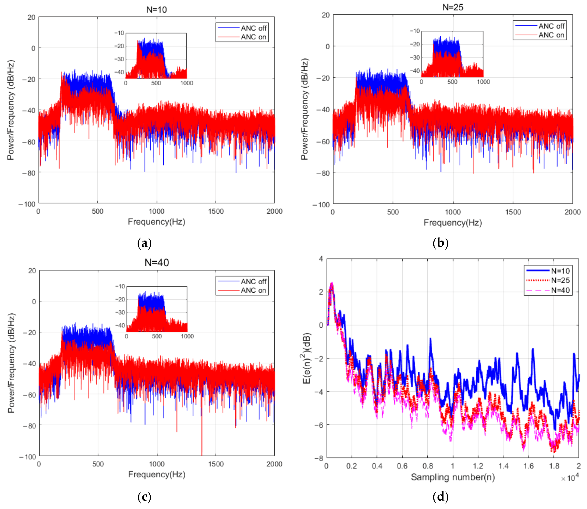
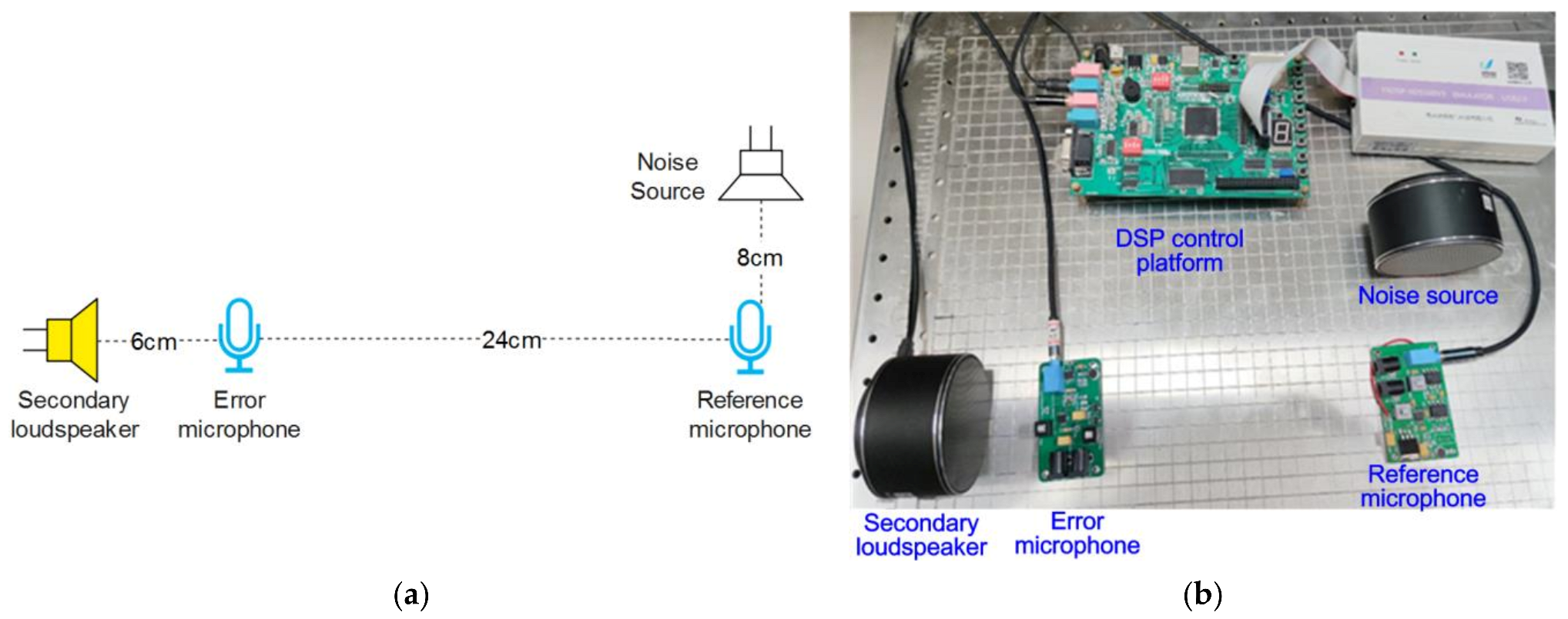
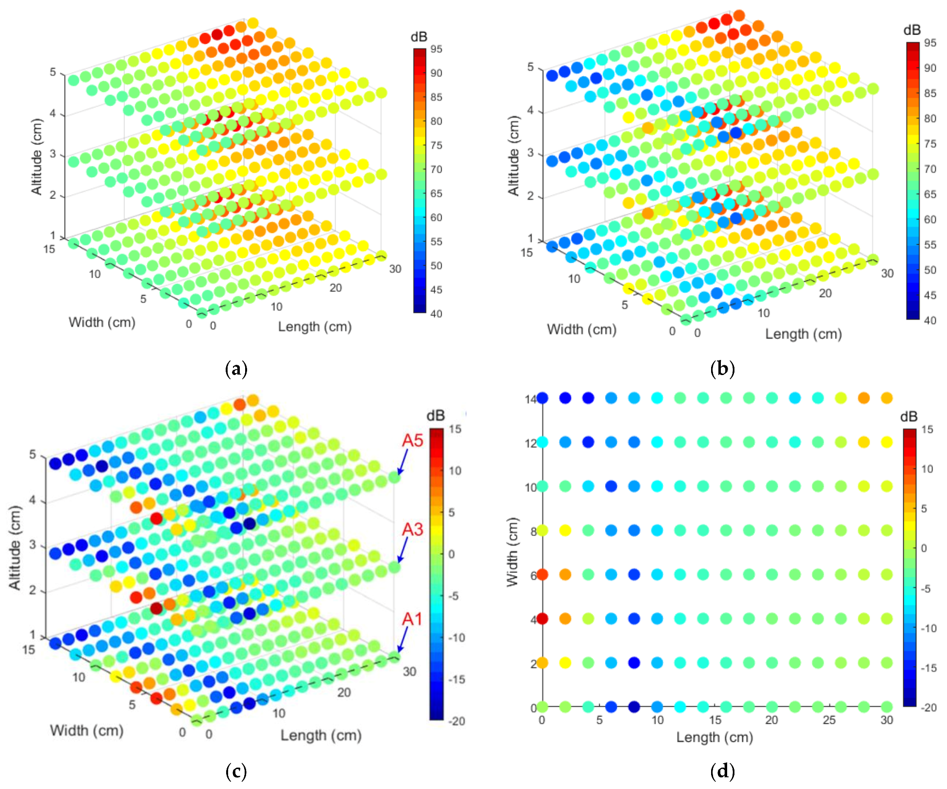
In this study, the stability of the online SPM system was analyzed in detail and the convergence conditions were derived when the relative error of the secondary path was large. The system can still converge stably at the start-up stage of the system operation or when the secondary path changes suddenly. The step-size upper bound of the ANC filter changes with the relative error of the auxiliary path, which can avoid the instability of the system caused by secondary path errors to a great extent. In addition, based on the model, a suitable step size for the ANC filter can be applied for various types of input signals. Finally, the steady-state MSE not having a closed-form expression is explained. Compared with the existing literature methods, the controller of the system is fitted online in all operating stages, without the need for offline fitting for a period of time, and when the mutation of the secondary path causes the relative error of the fitting filter to be large, the system can still have good stability. The simulation results verify the effectiveness of the model, ensure the stability of the system under different conditions, and have stronger robustness. The experimental results show that the ANC system had a noticeable noise reduction effect for different types of noise signals, and the noise reduction amount for more complex narrowband noise signals can reach 15 dB. The system can establish an effective quiet space in the local space, with an average noise reduction of approximately 15 dB and a maximum of 20 dB. These results have practical significance for other complex online secondary path modeling and local space noise reduction.

Author Contributions

Conceptualization, methodology, Y.L., Z.L., and W.Z.; software, validation, investigation, Y.L., Z.L., and Q.X.; writing—original draft preparation, Y.L.; resources, writing—review and editing, W.Z. All authors have read and agreed to the published version of the manuscript.

Funding

This research was funded by the national natural science foundation of China, grant number 61573073.

Institutional Review Board Statement

Not applicable.

Informed Consent Statement

Not applicable.

Data Availability Statement

The datasets used and/or analyzed during the current study are available from the corresponding author on reasonable request.

Acknowledgments

The authors would like to thank A. Carini for his valuable advice and the relevant data on this research.

Conflicts of Interest

The authors declare no conflict of interest.

Appendix A

We here investigate the evaluation of q w ( n + 1 ) .
q w ( n + 1 ) = q w ( n ) 2 μ w E ( Δ w T ( n ) ( A ( n ) + B ( n ) ) T Δ w ( n ) ) + μ w 2 E ( Δ w T ( n ) ( A ( n ) + B ( n ) ) T × ( A ( n ) + B ( n ) ) Δ w ( n ) ) + μ w 2 E ( b T ( n ) b ( n ) ) .
For the third term:
Δ w T ( n ) ( A ( n ) + B ( n ) ) T ( A ( n ) + B ( n ) ) Δ w ( n ) = | | Δ w T ( n ) ( A ( n ) + B ( n ) ) T ( A ( n ) + B ( n ) ) Δ w ( n ) | | | | Δ w T ( n ) | | | | ( A ( n ) + B ( n ) ) T ( A ( n ) + B ( n ) ) | | | | Δ w ( n ) | | = | | ( A ( n ) + B ( n ) ) T ( A ( n ) + B ( n ) ) | | | | Δ w T ( n ) | | | | Δ w ( n ) | | .
Using the definition of · :
Δ w ( n ) Δ w T ( n ) = max ( | Δ w i ( n ) | , 0 i N 1 ) × ( i = 0 N 1 | Δ w i ( n ) | ) N ( i = 0 N 1 Δ w i 2 ( n ) ) = N q w ( n ) .
Note, A ( n ) is a symmetric matrix:
| | ( A ( n ) + B ( n ) ) T ( A ( n ) + B ( n ) ) | |   | | ( A 2 ( n ) | | + | | B T ( n ) B ( n ) | | + | | A ( n ) B ( n ) | | + | | B T ( n ) A ( n ) | | .
The ( k . m ) -th ( 0 k , m N 1 ) entry of A ( n ) , B ( n ) is:
a k m ( n ) = j = 0 L 1 i = 0 L 1 ( s L 1 i s L 1 j x ( n i k ) x ( n j m ) ) ,
b k m ( n ) = j = 0 L 1 i = 0 L 1 ( Δ s L 1 i ( n ) s L 1 j x ( n i k ) x ( n j m ) ) .
The ( k 1 , m 1 ) -th ( 0 k 1 , m 1 N 1 ) entry of A 2 ( n ) is:
a k 1 m 1 ( n ) = q = 0 N 1 p = 0 N 1 a k 1 q a p m 1 = q = 0 N 1 p = 0 N 1 j = 0 L 1 i = 0 L 1 j 1 = 0 L 1 i 1 = 0 L 1 ( s L 1 i s L 1 j s L 1 i 1 s L 1 j 1 × x ( n i k 1 ) x ( n j q ) x ( n i 1 p ) x ( n j 1 m 1 ) ) N 2 σ x 4 ( j = 0 L 1 i = 0 L 1 s L 1 j 2 s L 1 i 2 + 2 i = 0 L 1 s L 1 i 4 ) 3 R 2 N 2 σ x 4 .
By (A7), it can derive that:
E ( a k 1 m 1 ( n ) ) N 2 σ x 4 ( j = 0 L 1 i = 0 L 1 s L 1 j 2 s L 1 i 2 + 2 i = 0 L 1 s L 1 i 4 ) 3 K 2 N 2 σ x 4 ,
E ( A 2 ) 3 R 2 N 3 σ x 4 .
The ( k 1 , m 1 ) -th ( 0 k 1 , m 1 N 1 ) entry of A ( n ) B ( n ) is:
c k 1 m 1 ( n ) = q = 0 N 1 p = 0 N 1 a k 1 q b p m 1 = q = 0 N 1 p = 0 N 1 j = 0 L 1 i = 0 L 1 j 1 = 0 L 1 i 1 = 0 L 1 ( s L 1 i s L 1 j Δ s L 1 i 1 s L 1 j 1 × x ( n i k 1 ) x ( n j q ) x ( n i 1 p ) x ( n j 1 m 1 ) ) ) .
By (10), it can be derived that:
E ( c k 1 m 1 ( n ) ) 3 N 2 σ x 4 ( j = 0 L 1 s L 1 j 2 i = 0 L 1 s L 1 i 2 + i = 0 L 1 Δ s L 1 i 2 i = 0 L 1 s L 1 i 2 ) 3 R N 2 σ x 4 ( R + ( P f ( n ) / σ υ 2 ) ) ,
E ( A ( n ) B ( n ) ) 3 R N 3 σ x 4 ( R + ( P f ( n ) / σ υ 2 ) ) ,
E ( | | B T ( n ) A ( n ) | | ) 3 R N 3 σ x 4 ( R + ( P f ( n ) / σ υ 2 ) ) .
The ( k 1 , m 1 ) -th ( 0 k 1 , m 1 N 1 ) entry of B 2 ( n ) is:
b k 1 m 1 ( n ) = q = 0 N 1 p = 0 N 1 b k 1 q b p m 1 = q = 0 N 1 p = 0 N 1 j = 0 L 1 i = 0 L 1 j 1 = 0 L 1 i 1 = 0 L 1 ( Δ s L 1 i s L 1 j Δ s L 1 i 1 s L 1 j 1 × x ( n i k 1 ) x ( n j q ) x ( n i 1 p ) x ( n j 1 m 1 ) ) ) .
By (A14), it can be derived that:
E ( b k 1 m 1 ( n ) ) N 2 σ x 4 ( j = 0 L 1 i = 0 L 1 s L 1 j 2 Δ s L 1 i 2 + 2 i = 0 L 1 Δ s L 1 i 2 s L 1 i 2 ) 3 N 2 σ x 4 ( j = 0 L 1 s L 1 j 2 ) ( i = 0 L 1 Δ s L 1 i 2 ) ,
E ( B 2 ) 3 R N 3 σ x 4 ( P f ( n ) / σ υ 2 ) .
For the second term, we can use the same idea and expression (37), (38) in the main body to obtain:
E ( Δ w T ( n ) ( A ( n ) + B ( n ) ) T Δ w ( n ) ) N ( P f ( n ) / σ υ 2 + 3 R ) σ x 2 q w ( n ) .

References

  1. Marburg, S. Developments in structural-acoustic optimization for passive noise control. Arch. Comput. Method Eng. 2002, 9, 291–370. [Google Scholar] [CrossRef]
  2. Kuo, S.M.; Morgan, D.R. Active noise control: A tutorial review. Proc. IEEE 1999, 87, 943–973. [Google Scholar] [CrossRef] [Green Version]
  3. Torresin, S.; Albatici, R.; Aletta, F.; Babich, F.; Oberman, T.; Kang, J. Acoustic Design Criteria in Naturally Ventilated Residential Buildings: New Research Perspectives by Applying the Indoor Soundscape Approach. Appl. Sci. 2019, 9, 24. [Google Scholar] [CrossRef] [Green Version]
  4. Giannella, V.; Branda, F.; Passaro, J.; Petrone, G.; Barbarino, M.; Citarella, R. Acoustic Improvements of Aircraft Headrests Based on Electrospun Mats Evaluated Through Boundary Element Method. Appl. Sci. 2020, 10, 5712. [Google Scholar] [CrossRef]
  5. Chu, Y.J.; Mak, C.M.; Zhao, Y.; Chan, S.C.; Wu, M. Performance analysis of a diffusion control method for ANC systems and the network design. J. Sound Vib. 2020, 475, 17. [Google Scholar] [CrossRef]
  6. Sohrabi, S.; Gomez, T.P.; Garbi, J.R. Suitability of Active Noise Barriers for Construction Sites. Appl. Sci. 2020, 10, 17. [Google Scholar] [CrossRef]
  7. Kuo, S.M.; Vijayan, D. A secondary path modeling technique for active noise control systems. IEEE Trans. Speech Audio Process. 1997, 5, 374–377. [Google Scholar] [CrossRef]
  8. Ahmed, S.; Akhtar, M.T. Gain Scheduling of Auxiliary Noise and Variable Step-Size for Online Acoustic Feedback Cancellation in Narrow-Band Active Noise Control Systems. IEEE ACM Trans. Audio Speech Lang. 2017, 25, 333–343. [Google Scholar] [CrossRef]
  9. Chan, S.C.; Chu, Y.J. Performance Analysis and Design of FxLMS Algorithm in Broadband ANC System With Online Secondary-Path Modeling. IEEE Trans. Audio Speech Lang. Process. 2012, 20, 982–993. [Google Scholar] [CrossRef] [Green Version]
  10. Yang, F.R.; Guo, J.F.; Yang, J. Stochastic analysis of the filtered-x LMS algorithm for active noise control. IEEE-ACM Trans. Audio Speech Lang. 2020, 28, 2252–2266. [Google Scholar] [CrossRef]
  11. Snyder, S.D.; Hansen, C.H. The effect of transfer-function estimation errors on the filtered-x LMS algorithm. IEEE Trans. Signal Process. 1994, 42, 950–953. [Google Scholar] [CrossRef]
  12. Morgan, D.R. AN ANALYSIS OF MULTIPLE CORRELATION CANCELLATION LOOPS WITH A FILTER IN THE AUXILIARY PATH. IEEE Trans. Acoust. Speech Signal Process. 1980, 28, 454–467. [Google Scholar] [CrossRef]
  13. Eriksson, L.J.; Allie, M.C. Use of random noise for online transducer modeling in an adaptive active attenuation system. J. Acoust. Soc. Am. 1989, 85, 797–802. [Google Scholar] [CrossRef] [Green Version]
  14. Carini, A.; Malatini, S. Optimal variable step-size NLMS algorithms with auxiliary noise power scheduling for feedforward active noise control. IEEE Trans. Audio Speech Lang. Process. 2008, 16, 1383–1395. [Google Scholar] [CrossRef]
  15. Ahmed, S.; Akhtar, M.T.; Zhang, X. Robust auxiliary-noise-power scheduling in active noise control systems with online secondary path modeling. IEEE Trans. Audio Speech Lang. Process. 2013, 21, 13. [Google Scholar] [CrossRef]
  16. Aslam, M.S.; Raja, M.A.Z. A new adaptive strategy to improve online secondary path modeling in active noise control systems using fractional signal processing approach. Signal Process. 2015, 107, 433–443. [Google Scholar] [CrossRef]
  17. Davari, P.; Hassanpour, H. Designing a new robust on-line secondary path modeling technique for feedforward active noise control systems. Signal Process. 2009, 89, 1195–1204. [Google Scholar] [CrossRef]
  18. Akhtar, M.T.; Abe, M.; Kawamata, M. Noise power scheduling in active noise control systems with online secondary path modeling. IEICE Electron. Express 2007, 4, 66–71. [Google Scholar] [CrossRef] [Green Version]
  19. Zhang, M.; Lan, H.; Ser, W. Cross-updated active noise control system with online secondary path modeling. IEEE Trans. Speech Audio Process. 2001, 9, 598–602. [Google Scholar] [CrossRef]
  20. Akhtar, M.T.; Abe, M.; Kawamata, M. A new variable step size LMS algorithm-based method for improved online secondary path modeling in active noise control systems. IEEE Trans. Audio Speech Lang. Process. 2006, 14, 720–726. [Google Scholar] [CrossRef] [Green Version]
  21. Bjarnason, E. Analysis of the filtered-X LMS algorithm. IEEE Trans. Speech Audio Process. 1995, 3, 504–514. [Google Scholar] [CrossRef]
  22. Tobias, O.J.; Bermudez, J.C.M.; Bershad, N.J. Mean weight behavior of the filtered-X LMS algorithm. IEEE Trans. Signal Process. 2000, 48, 1061–1075. [Google Scholar] [CrossRef]
  23. Ardekani, I.T.; Abdulla, W.H. On the convergence of real-time active noise control systems. Signal Process. 2011, 91, 1262–1274. [Google Scholar] [CrossRef]
  24. Zhang, M.; Lan, H.; Ser, W. On comparison of online secondary path modeling methods with auxiliary noise. IEEE Trans. Speech Audio Process. 2005, 13, 618–628. [Google Scholar] [CrossRef]
  25. Xiao, Y.G.; Ma, L.Y.; Hasegawa, K. Properties of FXLMS-Based Narrowband Active Noise Control With Online Secondary-Path Modeling. IEEE Trans. Signal Process. 2009, 57, 2931–2949. [Google Scholar] [CrossRef]
  26. Liu, J.A.; Xiao, Y.G.; Sun, J.W.; Xu, L. Analysis of Online Secondary-Path Modeling With Auxiliary Noise Scaled by Residual Noise Signal. IEEE Trans. Audio Speech Lang. Process. 2010, 18, 1978–1993. [Google Scholar] [CrossRef]
  27. Miyoshi, S.; Kajikawa, Y. Statistical-mechanical analysis of the fxlms algorithm with actual primary path. In 2015 IEEE International Conference on Acoustics, Speech, and Signal Processing; IEEE: New York, NY, USA, 2015; pp. 3502–3506. [Google Scholar]
  28. Miyoshi, S.; Kajikawa, Y. Statistical-Mechanics Approach to Theoretical Analysis of the FXLMS Algorithm. IEICE Trans. Fundam. Electron. Commun. Comput. Sci. 2018, E101A, 2419–2433. [Google Scholar] [CrossRef]
  29. Akhtar, M.T.; Abe, M.; Kawamata, M.; Nishihara, A. Online secondary path modeling in multichannel active noise control systems using variable step size. Signal Process. 2008, 88, 2019–2029. [Google Scholar] [CrossRef]
  30. Mazo, J.E. Independence theory of equalizer convergence. Bell Syst. Tech. J. 1979, 58, 963–993. [Google Scholar] [CrossRef]
  31. Kuo, S.M.; Morgan, D. Active Noise Control Systems: Algorithms and DSP Implementations; John Wiley & Sons, Inc.: New York, NY, USA, 1996. [Google Scholar]
Figure 1. ANC system with online SPM.
Applsci 12 00926 g001
Figure 2. The impulse responses of primary path and secondary path. (a) The impulse response of the primary path p 1 ( n ) ; (b) the impulse response of the primary path p 2 ( n ) ; (c) the impulse response of the secondary path s 1 ( n ) ; (d) the impulse response of the secondary path s 2 ( n ) .
Applsci 12 00926 g002
Figure 3. The white Gaussian input: (a) the relative modeling error Δ w ( n ) ( d B ) ; (b) the relative modeling error Δ s ( n ) ( dB ) ; (c) the time-varying step-size upper bound parameter μ w max ( n ) . The first-order AR process input: (d) the relative modeling error Δ w ( n ) ( d B ) ; (e) the relative modeling error Δ s ( n ) ( dB ) ; (f) the time-varying step-size upper bound parameter μ w max ( n ) .
Applsci 12 00926 g003
Figure 4. The white Gaussian input: (a) the relative modeling error Δ w ( n ) ( d B ) ; (b) the relative modeling error Δ s ( n ) ( dB ) ; (c) the time-varying step-size upper bound parameter μ w max ( n ) . The first-order AR process input: (d) the relative modeling error Δ w ( n ) ( d B ) ; (e) the relative modeling error Δ s ( n ) ( dB ) ; (f) the time-varying step-size upper bound parameter μ w max ( n ) .
Applsci 12 00926 g004aApplsci 12 00926 g004b
Figure 5. The white Gaussian input: (a) the relative modeling error Δ w ( n ) ( d B ) ; (b) the time-varying step-size upper bound parameter μ w max ( n ) . The first-order AR process input: (c) the relative modeling error Δ w ( n ) ( d B ) ; (d) the time-varying step-size upper bound parameter μ w max ( n ) .
Applsci 12 00926 g005
Figure 6. Comparison of noise reduction performance when the reference signal is 400 Hz. (a) The order of the ANC filter is 10; (b) the order of the ANC filter is 20; (c) the order of the ANC filter is 30; (d) power changes in error microphone signal e(n) at different ANC filter orders.
Applsci 12 00926 g006
Figure 7. Comparison of noise reduction performance when the reference signal is multi-harmonic. (a) ANC filter order is 20; (b) ANC filter order is 30; (c) ANC filter order is 40; (d) the power change in error microphone signal e(n) when ANC filter order is different.
Applsci 12 00926 g007
Figure 8. Comparison of noise reduction performance when the reference signal is 200–600 Hz narrowband signal. (a) The order of the ANC filter is 10; (b) the order of the ANC filter is 25; (c) the order of the ANC filter is 40; (d) the power change in error microphone signal e(n) when the order of ANC filter is different.
Applsci 12 00926 g008
Figure 9. Experimental scene. (a) Schematic diagram; (b) experimental scene diagram.
Applsci 12 00926 g009
Figure 10. Spatial sound pressure distribution before and after noise reduction. (a) ANC off; (b) ANC on; (c) noise reduction amount; (d) mean value distribution of sound pressure on the same horizontal plane.
Applsci 12 00926 g010
Publisher’s Note: MDPI stays neutral with regard to jurisdictional claims in published maps and institutional affiliations.

