
A Filtering Method for Suppressing the Lift-Off Interference in Magnetic Flux Leakage Detection of Rail Head Surface Defect


Abstract
:1. Introduction
2. Related Works
3. Filtering Method
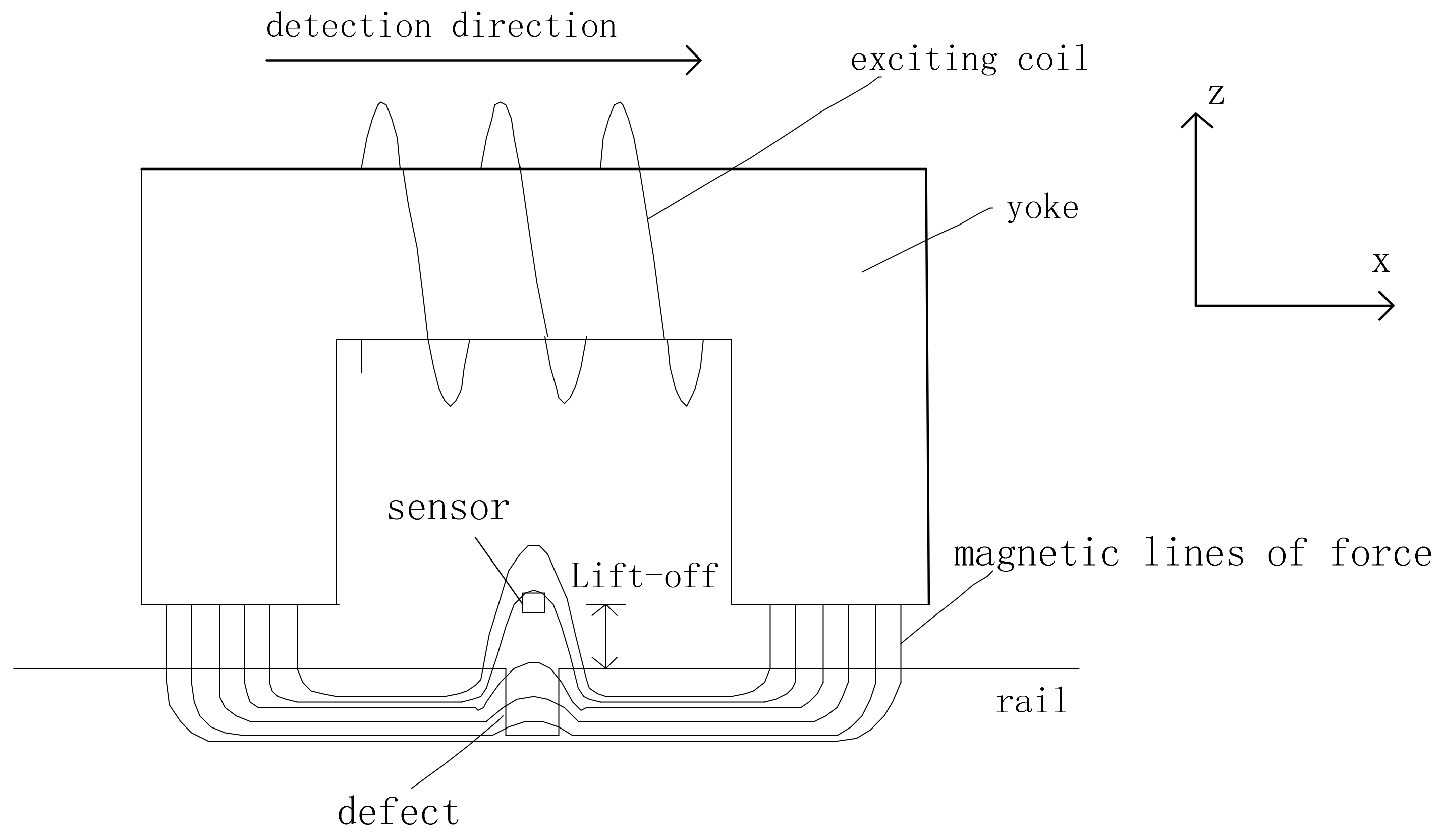
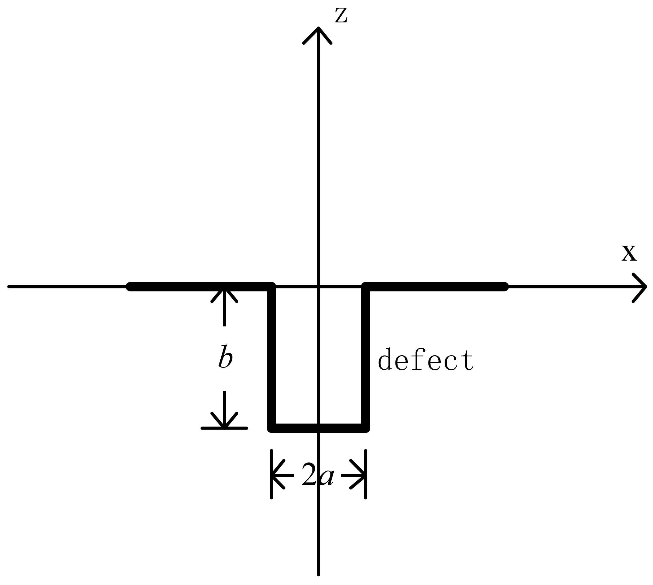
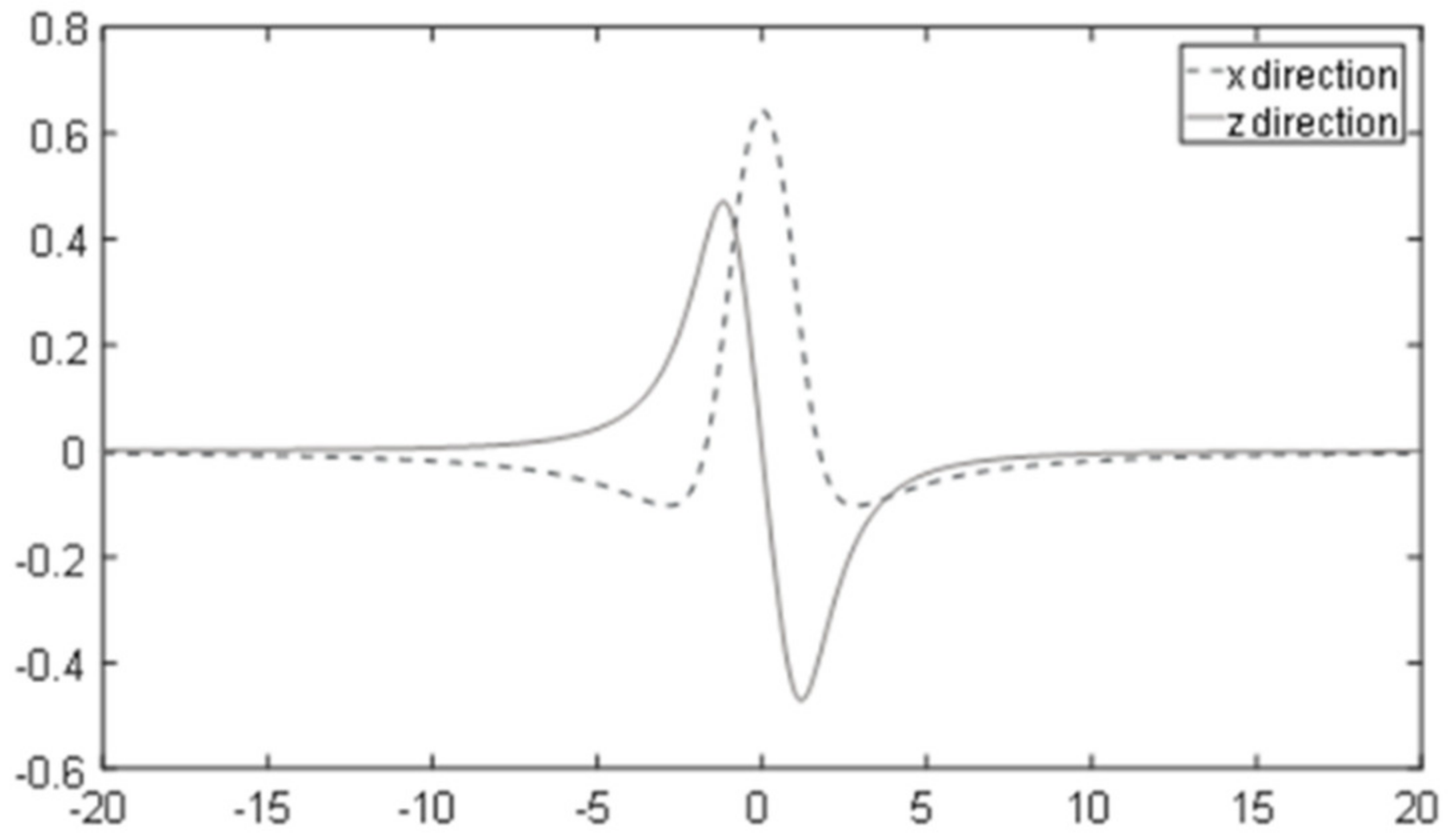
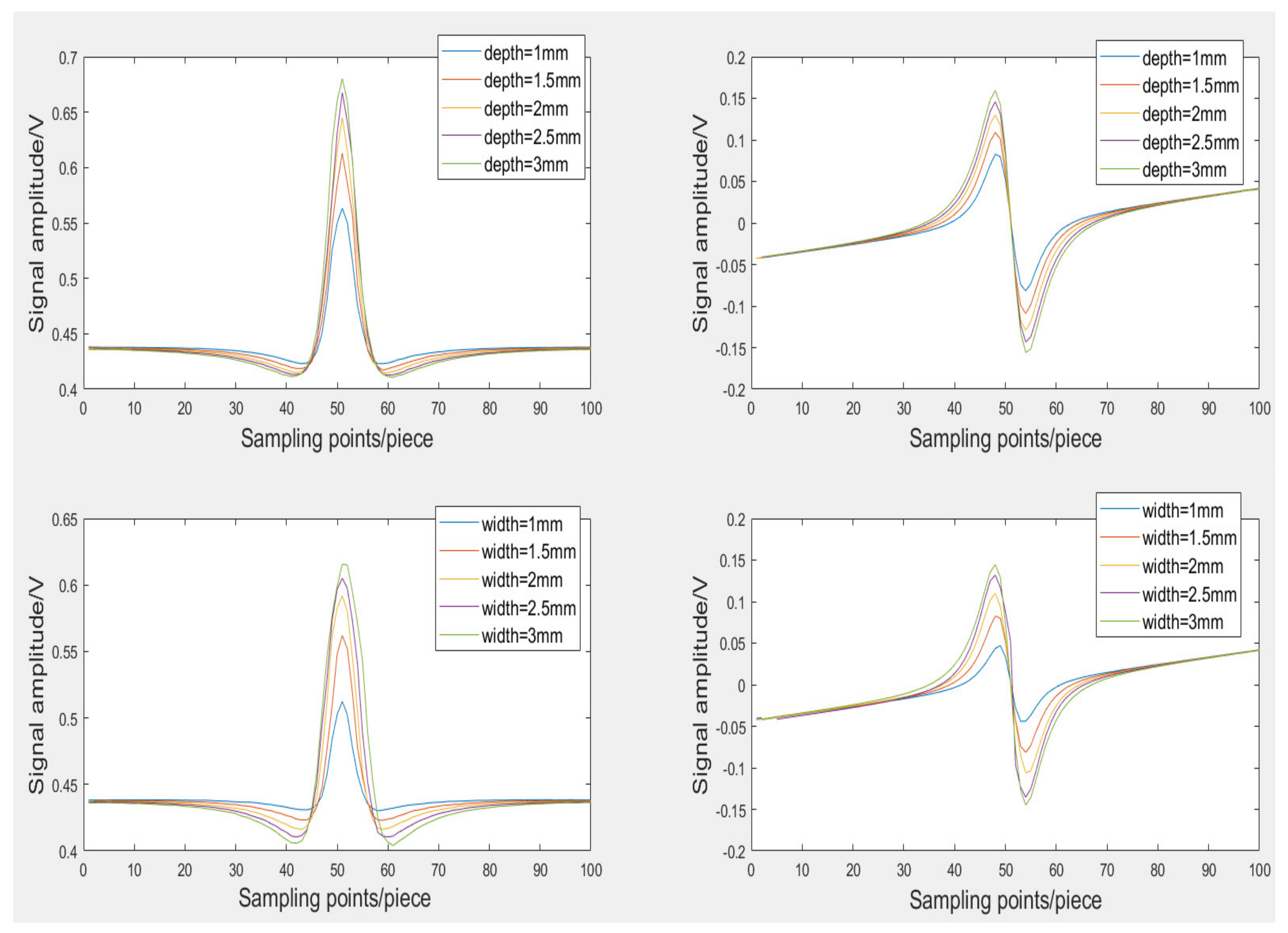
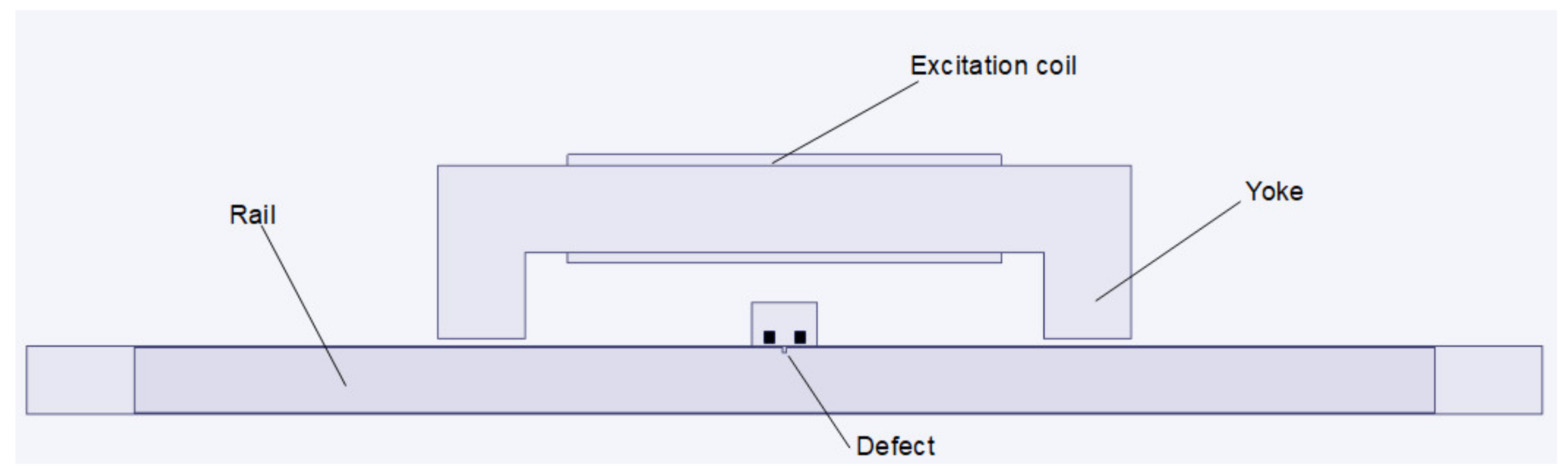
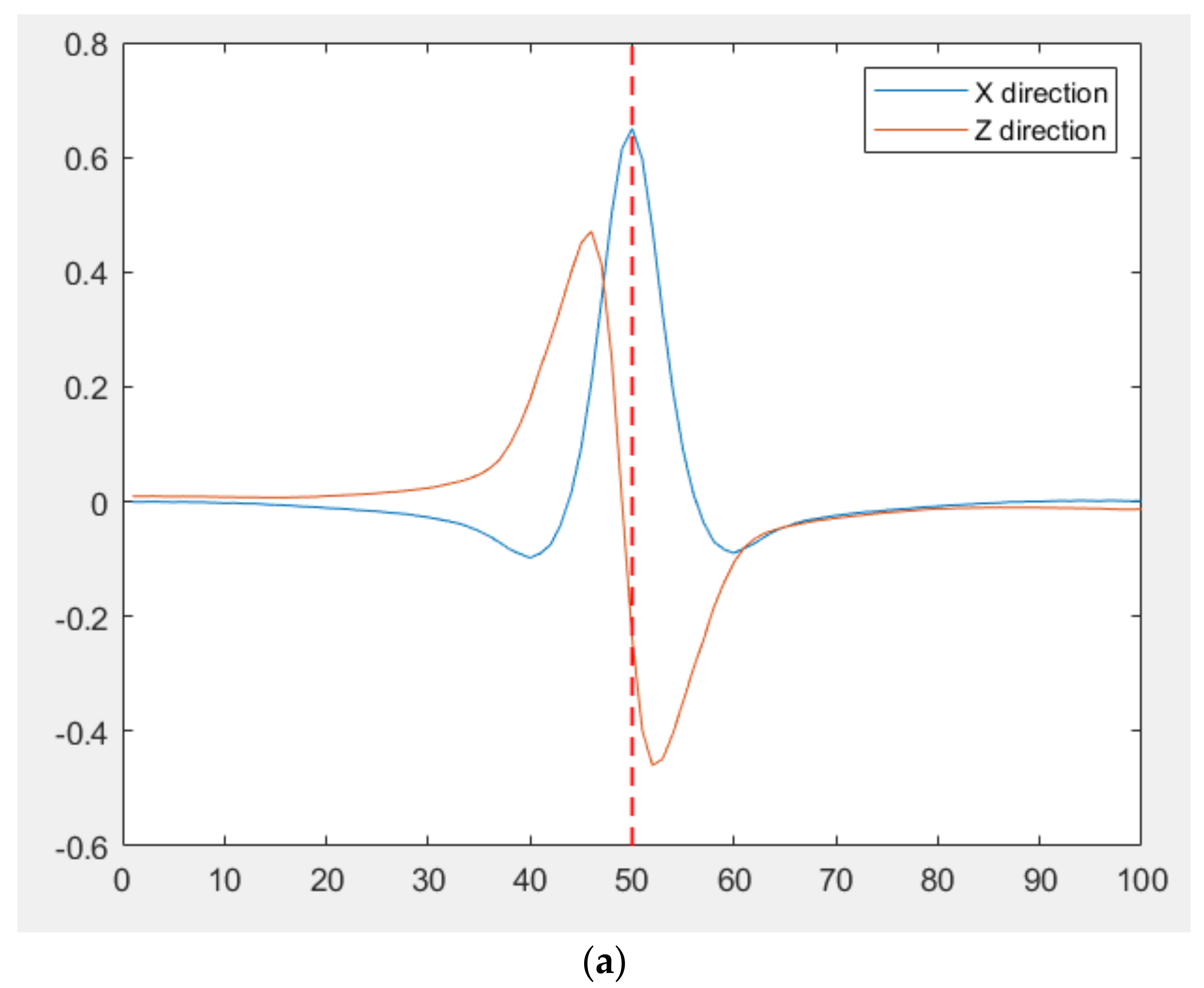
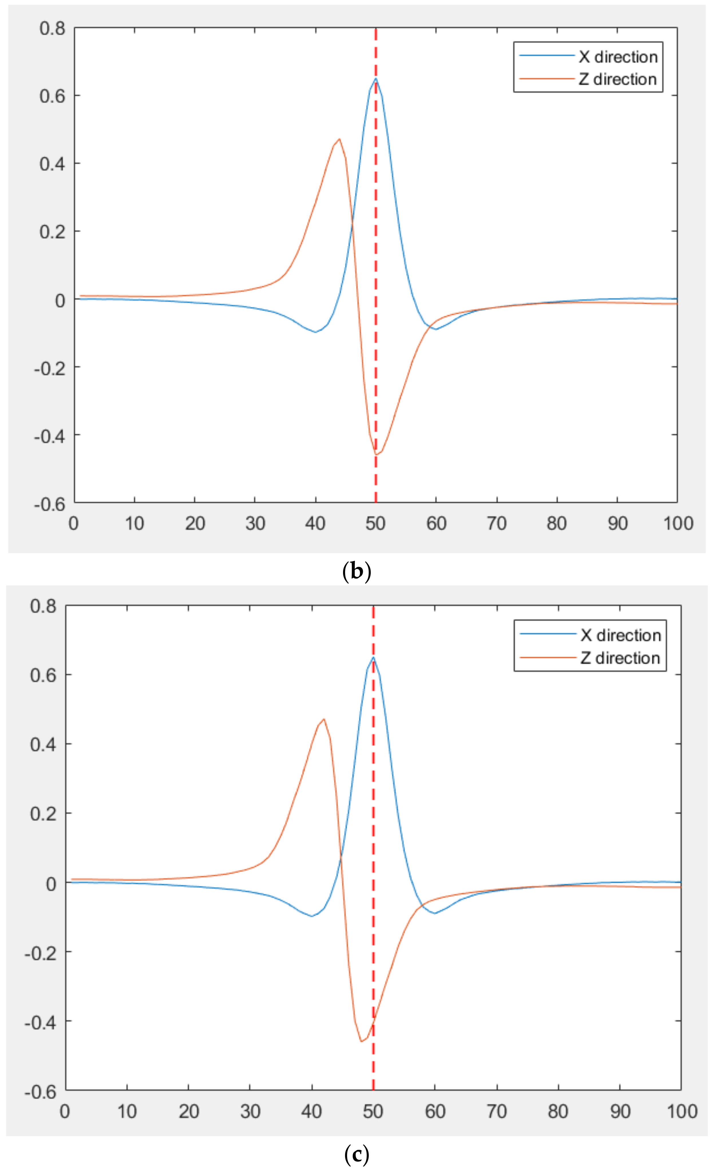
3.1. MFL Analysis
3.2. Principle of Filtering Method
3.3. Filtering Algorithm
- 1.
- Each sensor output is sampled, and the number of sampling points is denoted by M. The sampling results of Sx[i] and Sz[i] are array Sx[i,j] and Sz[i,j] (j = 1, 2, …, M).
- 2.
- The array and is calculated:q is a loop variable with an initial value of B + 1.
- 3.
- .
- 4.
- The minimum in (i = 1, 2, …, N) is found. The number of the pair that has the minimum is denoted by i0. The sampling point of the pair sensors are taken as the reference signal. , (i = 1, 2,…, N): The differences are taken as the filtering results of each sensor at this sampling point.
- 5.
- q = q + 1. If q ≤ M + B, the process returns to step 3, otherwise the filtering ends.
4. Experimental Results and Analysis
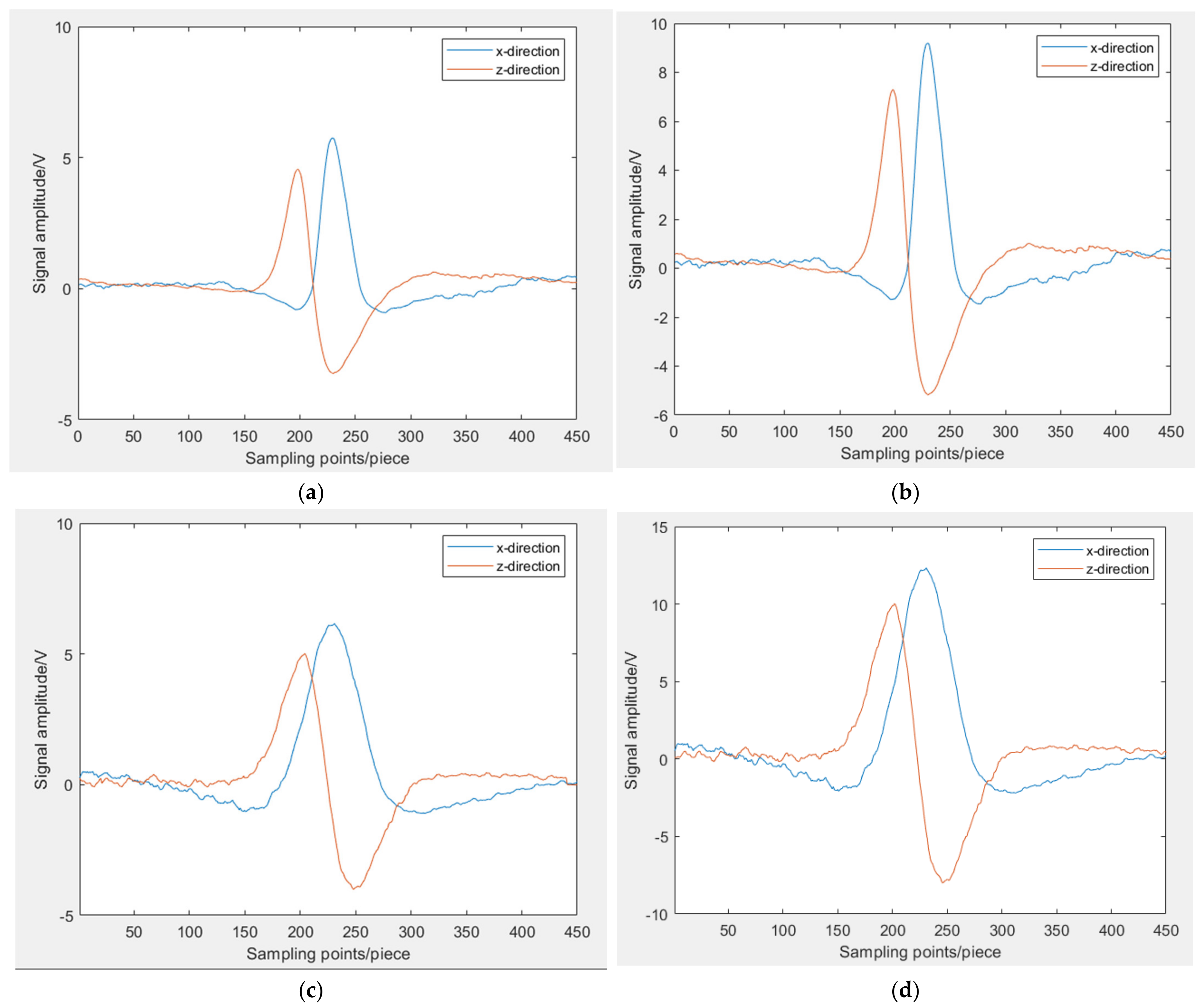
4.1. Finite Element Simulation Results and Analysis
4.2. Physical Experiment Results and Analysis
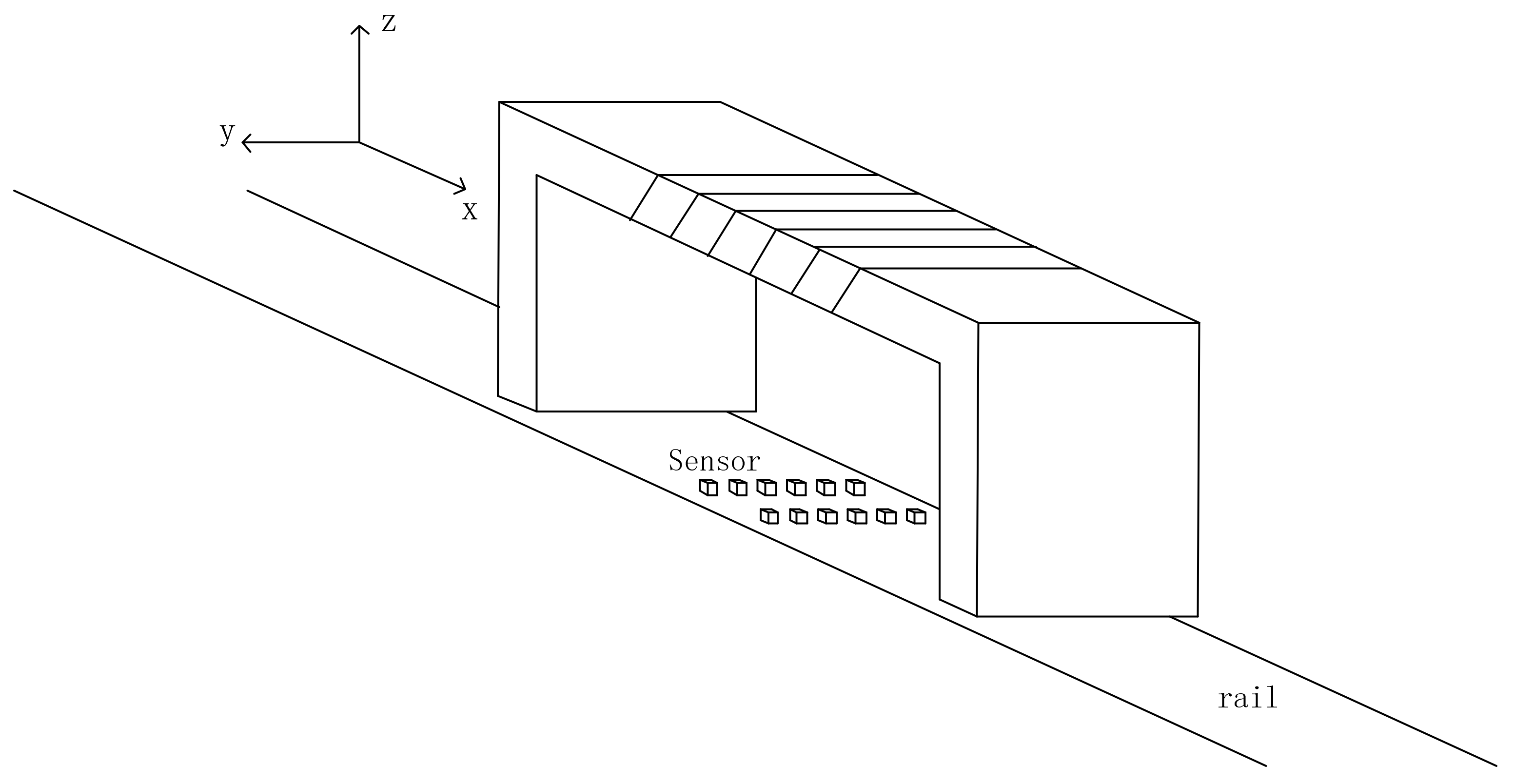
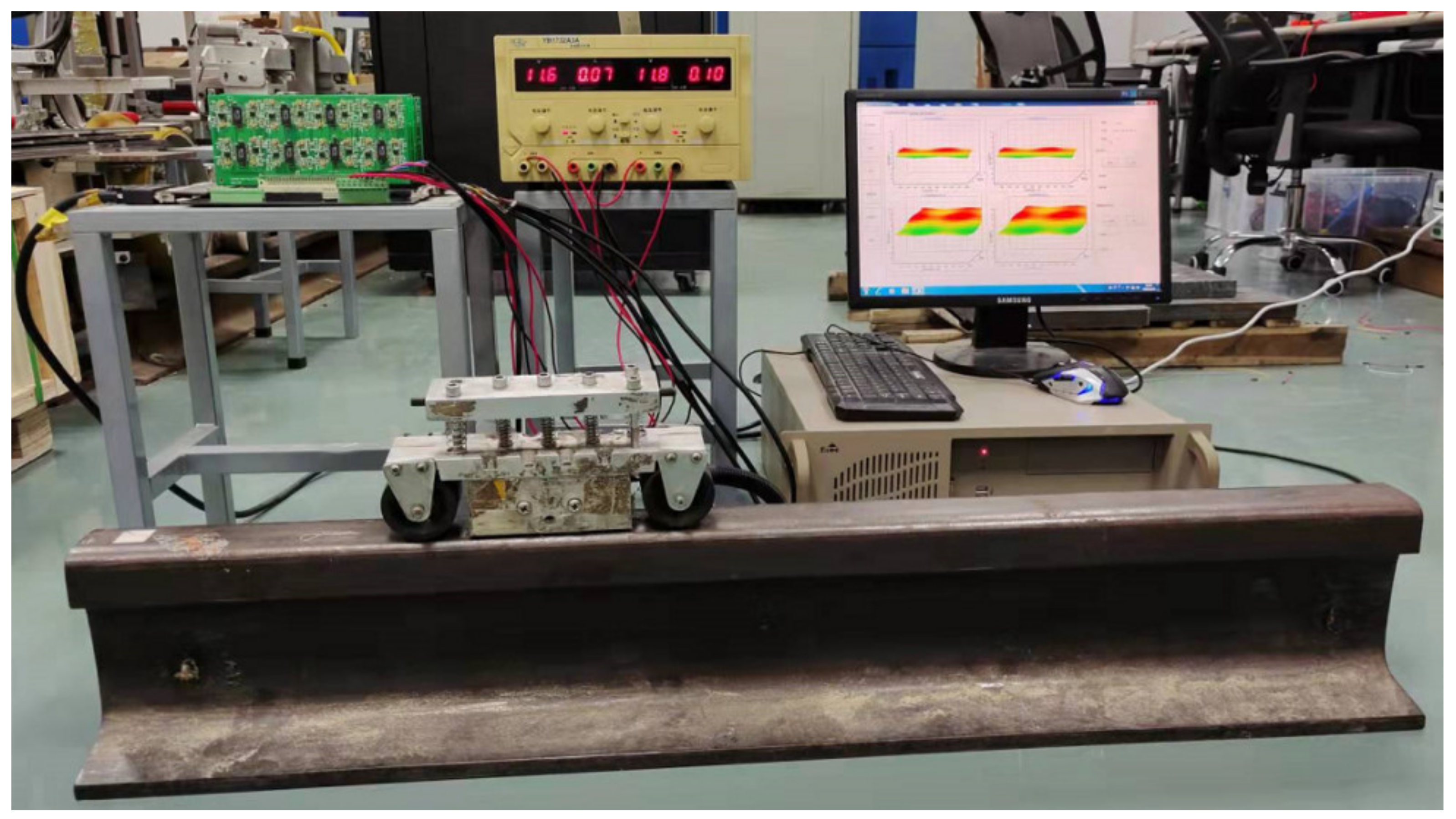
4.2.1. Experiment System
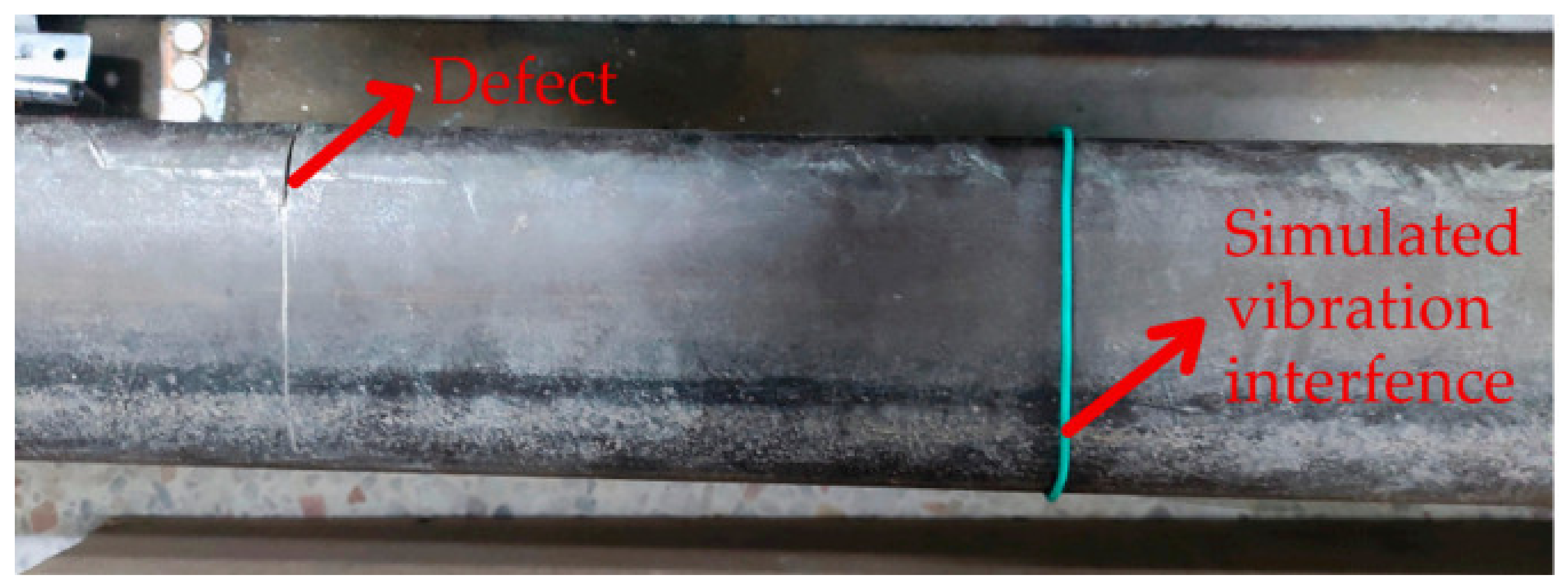
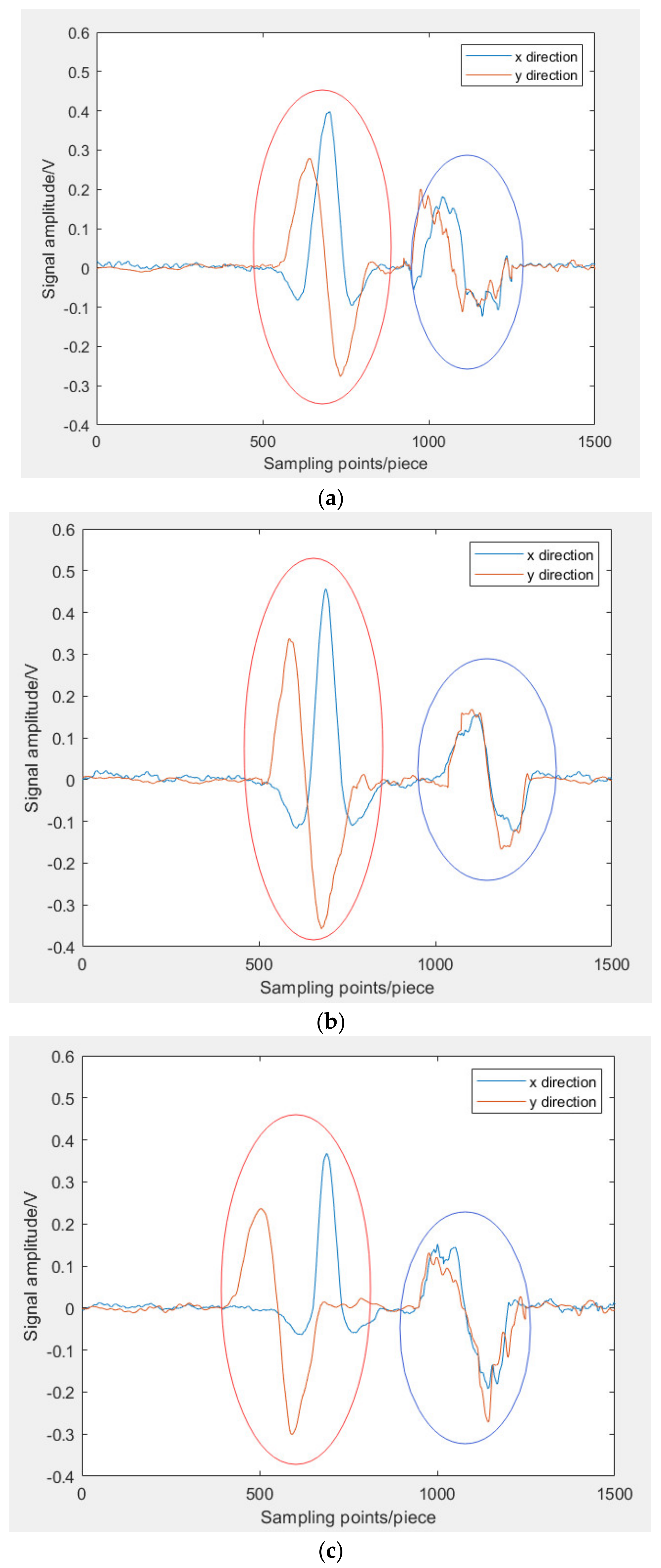
4.2.2. Single Defect Experiment
4.2.3. Multiple Defects Experiment
5. Conclusions
Author Contributions
Funding
Institutional Review Board Statement
Informed Consent Statement
Conflicts of Interest
References
- Zhang, H.; Song, Y.N.; Wang, Y.N. Review of rail defect non-destructive testing and evaluation. Chin. J. Sci. Instrum. 2019, 40, 11–25. [Google Scholar]
- Alahakoon, S.; Sun, Y.Q.; Spiryagin, M.; Cole, C. Rail Flaw Detection Technologies for Safer, Reliable Transportation: A Review. J. Dyn. Syst. Meas. Control 2018, 140, 020801. [Google Scholar] [CrossRef]
- Fu, L.Z.; Wu, J.J.; Lang, X.W. Experiment research on switch rail defect monitoring using ultrasonic guided waves. Railway Engineering 2018, 31, 129–133. [Google Scholar]
- Miki, M.; Ogata, M. Phased array ultrasonic testing methods for welds in bogie frames of railway vehicles. Insight 2015, 57, 382–388. [Google Scholar] [CrossRef]
- Hu, Q.W.; Wang, X.B.; Wu, W. Eddy current testing and evaluation method for fine cracks on rail surface. Equip. Manag. Maint. 2021, 42, 34–35. [Google Scholar]
- Wilson, J.W.; Tian, G.Y. 3D magnetic field sensing for magnetic flux leakage defect characterisation. Insight 2006, 48, 357–359. [Google Scholar] [CrossRef]
- Gao, L. Research on Image Detection and Recognition Method of Steel Plate Surface Defect Based on Magnetic Flux Leakage Signal. Master’s Thesis, Northeastern University, Shen Yang, China, 2017. [Google Scholar]
- Azari, H.; Al Ghorbanpoor; Shams, S. Development of Robotic Nondestructive Testing of Steel Corrosion of Prestressed Concrete Bridge Girders using Magnetic Flux Leakage System. Transp. Res. Record. 2020, 2674, 466–476. [Google Scholar] [CrossRef]
- Peng, X.; Anyaoha, U.; Tsukada, K. Analysis of Magnetic-Flux Leakage(MFL) Data for Pipeline Corrosion Assessment. IEEE Trans. Magn. 2020, 57, 6200410. [Google Scholar] [CrossRef]
- Piao, G.Y.; Guo, J.B.; Hu, T.H.; Leung, H.; Deng, Y.M. Fast reconstruction of 3-D defect profile from MFL signals using key physics-based parameters and SVM. NDT E Int. 2019, 103, 26–38. [Google Scholar] [CrossRef]
- Wu, D.H.; Su, L.X.; Wang, X.H. A Novel Non-destructive Testing Method by Measuring the Change Rate of Magnetic Flux Leakage. J. Nondestruct. Eval. 2017, 36, 24. [Google Scholar]
- Usarek, Z.; Chmielewski, M.; Piotrowski, L. Reduction of the Velocity Impact on the Magnetic Flux Leakage Signal. J. Nondestruct. Eval. 2019, 38, 28. [Google Scholar] [CrossRef] [Green Version]
- Feng, B.; Kang, Y.H.; Sun, Y.H. Magnetization Time Lag Caused by Eddy Currents and Its Influence on High-Speed Magnetic Flux Leakage Testing. Res. Nondestruct. Eval. 2019, 30, 189–204. [Google Scholar] [CrossRef]
- Karuppasamy, P.; Abudhahir, A.; Jayakumar, T. Model-Based Optimization of MFL Testing of Ferromagnetic Steam Generator Tubes. J. Nondestruct. Eval. 2016, 35, 5. [Google Scholar] [CrossRef]
- Watson, J.M.; Liang, C.W.; Sexton, J.; Missous, M. Magnetic field frequency optimisation for MFL imaging using QWHE sensors. Insight 2020, 62, 396–401. [Google Scholar] [CrossRef]
- Zhang, O.; Wei, X.Y. De-noising of Magnetic Flux Leakage Signals Based on Wavelet Filtering Method. Res. Nondestruct. Eval. 2019, 30, 269–286. [Google Scholar] [CrossRef]
- Liu, S.W.; Sun, Y.H.; Deng, Z.Y.; He, L.S. A novel method of omnidirectional defects detection by MFL testing under single axial magnetization at the production stage of lathy ferromagnetic materials. Sens. Actuator A-Phys. 2017, 262, 35–45. [Google Scholar] [CrossRef]
- Liu, X.C.; Wang, Y.J.; Wu, B.; He, C.F. Design of Tunnel Magnetoresistive-Based Circular MFL Sensor Array for the Detection of Flaws in Steel Wire Rope. J. Sens. 2016, 6, 198065. [Google Scholar]
- Wu, D.H.; Liu, Z.T.; Su, L.X. New MFL detection method based on differential peak extraction using dual sensors. Chin. J. Sci. Instrum. 2016, 37, 1218–1225. [Google Scholar]
- Ding, S.Y. Research on De-Noising and Recognition of Rail Magnetic Flux Leakage Signal Based on Adaptive Filtering and Random Forest. Master’s Thesis, Nanjing University of Aeronautics and Astronautics, Nan Jing, China, 2020. [Google Scholar]
- Ji, K.L.; Wang, P.; Jia, Y.L.; Ye, Y.F.; Ding, S.Y. Adaptive Filtering Method of MFL Signal on Rail Top Surface Defect Detection. IEEE Access 2021, 9, 87351–87359. [Google Scholar] [CrossRef]
- Jia, Y.L.; Zhang, S.C.; Wang, P.; Ji, K.L. A Method for Detecting Surface Defects in Railhead by Magnetic Flux Leakage. Appl. Sci. 2021, 11, 9489. [Google Scholar] [CrossRef]


| Defect 1 | Defect 2 | Defect 3 | Defect 4 | Defect 5 | Defect 6 | Defect 7 | Defect 8 | |
|---|---|---|---|---|---|---|---|---|
| Width | 2.0 mm | 2.2 mm | 2.2 mm | 2.5 mm | 2.5 mm | 2.5 mm | 2.5 mm | 2.5 mm |
| Depth | 1.0 mm | 1.2 mm | 1.2 mm | 2.0 mm | 2.5 mm | 2.5 mm | 2.8 mm | 3.0 mm |
Publisher’s Note: MDPI stays neutral with regard to jurisdictional claims in published maps and institutional affiliations. |
© 2022 by the authors. Licensee MDPI, Basel, Switzerland. This article is an open access article distributed under the terms and conditions of the Creative Commons Attribution (CC BY) license (https://creativecommons.org/licenses/by/4.0/).
Share and Cite
Jia, Y.; Lu, Y.; Xiong, L.; Zhang, Y.; Wang, P.; Zhou, H. A Filtering Method for Suppressing the Lift-Off Interference in Magnetic Flux Leakage Detection of Rail Head Surface Defect. Appl. Sci. 2022, 12, 1740. https://0-doi-org.brum.beds.ac.uk/10.3390/app12031740
Jia Y, Lu Y, Xiong L, Zhang Y, Wang P, Zhou H. A Filtering Method for Suppressing the Lift-Off Interference in Magnetic Flux Leakage Detection of Rail Head Surface Defect. Applied Sciences. 2022; 12(3):1740. https://0-doi-org.brum.beds.ac.uk/10.3390/app12031740
Chicago/Turabian StyleJia, Yinliang, Yichen Lu, Longhui Xiong, Yuhua Zhang, Ping Wang, and Huangjian Zhou. 2022. "A Filtering Method for Suppressing the Lift-Off Interference in Magnetic Flux Leakage Detection of Rail Head Surface Defect" Applied Sciences 12, no. 3: 1740. https://0-doi-org.brum.beds.ac.uk/10.3390/app12031740