
Efficient Fake News Detection Mechanism Using Enhanced Deep Learning Model
by
 , , and
Tahir Ahmad
1, 
Muhammad Shahzad Faisal
1,*,
Atif Rizwan
2 ,
,
Reem Alkanhel
3,*,
Prince Waqas Khan
2 and
and
Ammar Muthanna
4,5
1
Department of Computer Science, Attock Campus, COMSATS University Islamabad, Attock 43600, Pakistan
2
Department of Computer Engineering, Jeju National University, Jejusi 63243, Korea
3
Department of Information Technology, College of Computer and Information Sciences, Princess Nourah bint Abdulrahman University, P.O. Box 84428, Riyadh 11671, Saudi Arabia
4
Department of Telecommunication Networks and Data Transmission, The Bonch-Bruevich Saint-Petersburg State University of Telecommunications, 193232 Saint Petersburg, Russia
5
Department of Applied Probability and Informatics, Peoples’ Friendship University of Russia (RUDN University), 117198 Moscow, Russia
*
Authors to whom correspondence should be addressed.
Appl. Sci. 2022, 12(3), 1743; https://0-doi-org.brum.beds.ac.uk/10.3390/app12031743
Submission received: 17 December 2021
/
Revised: 29 January 2022
/
Accepted: 30 January 2022
/
Published: 8 February 2022
(This article belongs to the Special Issue Natural Language Processing: Recent Development and Applications)
Abstract
:The spreading of accidental or malicious misinformation on social media, specifically in critical situations, such as real-world emergencies, can have negative consequences for society. This facilitates the spread of rumors on social media. On social media, users share and exchange the latest information with many readers, including a large volume of new information every second. However, updated news sharing on social media is not always true.In this study, we focus on the challenges of numerous breaking-news rumors propagating on social media networks rather than long-lasting rumors. We propose new social-based and content-based features to detect rumors on social media networks. Furthermore, our findings show that our proposed features are more helpful in classifying rumors compared with state-of-the-art baseline features. Moreover, we apply bidirectional LSTM-RNN on text for rumor prediction. This model is simple but effective for rumor detection. The majority of early rumor detection research focuses on long-running rumors and assumes that rumors are always false. In contrast, our experiments on rumor detection are conducted on real-world scenario data set. The results of the experiments demonstrate that our proposed features and different machine learning models perform best when compared to the state-of-the-art baseline features and classifier in terms of precision, recall, and F1 measures.
1. Introduction
The social media platform is rapidly growing day by day. The pew research center [1] stated that in august 2017, 67% of Americans received new information from social media platforms and 74% of twitter users obtained their news from the website. Social media networks, especially twitter, is the primary source of posting and sharing the latest updates that come from the fact that anyone can share. Twitter has a monthly active social media presence of 330 million and a daily active number of users of approximately 145 million. Twitter demographic background age shows that 63% of twitter users are between the ages of 35 and 65, while the twitter demographic gender shows that 34% of twitter users are female and 66% are male [2]. In social media platforms, users share and exchange the latest information with many readers, including a large volume of new information every second. However, updated news sharing on social media is not always true. One most popular example reported by a single rumor tweet was “Two explosions in the white house and Barack Obama is injured” in 2013. However, that rumor was the most popular in only six minutes [3]. This and many more examples illustrate how rumors posted on social media can have a harmful impact on individuals and society. The example of societal issues [3] is finding latest breaking news on social media. Today, it is possible to spread information or news in real time with other people by using internet-connected devices. Hence, it is a powerful tool for journalists is social media as well as for other ordinary citizens [4]. However, social media provide access to spreading misinformation which then requires lots of significant effort to maintain the presence and veracity [5]. The updated news related to breaking news is posted by an initiator that is not confirmed at posting. Later, it can be proven that the breaking news is true or false [6]. The term for news that is not confirmed when posting is called “rumor”. Some recent work defined rumors as follows: “rumor is collection of information that is deemed false” [7]. Most works in the literature explain that “unverified and instrumentally relevant information statement is circulation” [8]. There are different types of factors available that describe the type of rumor, including the veracity value (true, false, unresolved) [9]. Another classification type of rumors describes the three types of rumors: (i) pipe-dream rumor, which depends on wishful thinking; (ii) “boggy” rumors, which increase the anxiety of the rumor; and (iii) “wedge dowry” rumor, which is a rumor that generates hatred.
In this research article, we deeply study the problems of automatically finding rumors in social media. This research uses a new set of content-based and social-based features for rumor detection. We also apply a deep learning model on text data using a bidirectional LSTM-RNN classifier. In this paper, our main contribution is as follows. We compute different types of new features using twitter as a social media network for rumor detection. In this research work, we also apply a deep learning model that is Bi LSTM-RNN on text data of different events of data sets for rumor prediction. Finally, we compare the results of our proposed features and classifier with the baseline features set and model. Our proposed features perform best in terms of precision, recall, and F1.
For all of the data provided, this study examines the spreading patterns of both rumors and non-rumors by first extracting temporal aspects. The data for this research were taken from the PHEME data set, which is a publicly available. Figure 1 show the annual twitter users from 2010 to 2018. from figure The X-axis represents the time interval. Because this study endeavors to consider tweets made within an hour of the originating tweet, it is in the second format. The Y-axis represents the number of interactions per second. As can be observed, the number of interactions for rumors is lower than the number of interactions for non-rumors for the vast majority of events. It is difficult to tell the difference between rumors and facts by using Ottawa shooting and the Germanwings crash.
2. Related Work
The goal of this study is to find out how to detect real-life rumors that spread on twitter. Related work includes real-world emergencies, fake news detection, and some NLP are used. Our work is on the dissemination and propagation of information in social networks, on twitter, and other domains from the discipline of network science.
2.1. Rumor Detection
Rumor detection has been a hot issue of embedding in recent years, and there are two approaches used to propose solutions: model based or feature based. In some papers, multiple features are proposed, i.e., content features and social context features or network features, while in some papers, the best algorithms are discussed to find out rumors. In article [10], they addressed two basic problems. The first issue is retrieving rumor-related micro blogs on the internet. The second difficulty is to find tweets that supported the rumor. They evaluated the effectiveness of three extracted features: content-based features, network-based features, and micro blog features. They used specific memory for the correct classification of rumors. They performed manually 10,000 experiments on the tweet and represented how their related model achieves more than 0.95 on the map. This shows that this data set is one of the largest data sets on rumors detection. In [11], the authors proposed a new model for the detection of rumors on twitter in 2012. In that literature work, they described how rumors spread after an earthquake disaster and discussed how we can deal with those types of rumors. They first investigated the actual instance of a rumor that was generated after a disaster, and they attempted to disclose the rumor characteristics. They designed a model system that can detect candidates of rumors from twitter based on the investigation. They extracted tweets that contain the keyword “server room” or geek “how and “come oil” for r1 and r2 data sets, and they manually checked in order to remove irrelevant tweets to obtain 1135 tweets from r1 and 242 tweets from r2. In this research, the author used the (SPADE) [12] social spam analysis and detection framework across more than one social network to show the flexibility and efficiency of the cross down classification. They produced the results on large-scale study web pages, email spam, for an extended period. They used these basic models: first is the profile-based model, the second is the message-based model, and the last one is the web page model in SPADE. All the models represent the most critical object on the social network. The data of all models are stored in XML because of the extensibility and scalability of the models. They use the F measure and accuracy evaluation for the result. The proposed classifier improves the accuracy by 7% and FP rate above 20%.
A model for automatically detecting rumors on social media networks was proposed [13]. The authors used implicit content-based and user-based features, such as popularity orientation, external and internal consistency, sentimental polarity, and the degree of match of the message. Features selection was the most critical work in this paper. Their work contained three-part data cleansing, feature extraction, and model training. In the data cleaning process, they filtered out spam messages, such as other old features. After features selection, they applied the classifier with SVM and random forest classifier. Finally, they showed their improvement in precision and recall.
Correctly rumor identification and belief investigation on social media networks, such as twitter, were proposed [14] in 2016. In this literature, they attempted to solve the problem of rumor detection on the twitter platform. They extracted two new features in their proposed model: first is addressing the missing word and latency issues (TLV), and the second is user belief about each rumor. The SVM tree kernel model 5 was applied to it for the detection of rumors. To check the proof of another classifier of other classifier, including j48, NB, the proposed performance is better. In this research, the detection of rumors using the supervised machine learning technique on twitter data was proposed [15]. They used a two-fold supervised machine learning approach for the detection of rumors. They applied multiple models, such as Naïve Bayes, Support Vector Machine (SVM), etc., to achieve an accuracy of 81%. Finally, using textual data characteristics, rumors were detected using cleaning data.
In the article [16], the author proposed a method of rumor detection based on SDSMOTE and feature selection in 2019. In this paper, they detected rumors in the specific topic using Sina micro blogs, and six new features were added; with guide less words (suspicious, topic, recognition of information, degree of attention to the user, and credit ranking), they used the SMODE algorithm to reduce the impact of unbalanced data. They detected 90% of rumors with an acceptable level of precision. Ref. [17] presented a novel approach for rumor detection that contains new features, including bias potential and measuring the characteristics of the network. They tested their model on a real data set that contains all posts related to health collected from the twitter network. Experimental result showed that using new features correctly detects 90% of rumors with acceptable precision. They also used different classifiers for the selection of different features for rumor detection, which is beneficial for the future selection for best classifier and effective features.
Authors in [18] used long short-term memory (LSTM) for the detection of online rumors. They captured the long short-term memory (LSTM) with a neural network for rumor detection based on content that is of a forwarding, spreader, and diffusion structure. For forwarding content, they used a word embedding model for the representation of words. For spreader content, they captured the popularity of content that is forward [19]. For diffusion, they proposed to change the structure of the diffusion layer and change the model between different layers of diffusion [20]. The final data set contains 1623 rumors and 1756 non-rumor. They evaluated the experimental results with the baseline paper by using accuracy and F1 measure as the parameters. This analysis [21] introduced and discussed two types of rumors that spread on social media. One is a long-standing rumor that circulates for a long period of time, and the second is newly emerging rumors spawned during fast-paced events, such as breaking news, where reports are shared without any verification. They provided an overview of a rumor classification system that consists of four components: first is rumor detection, second is rumor tracking, third is rumor stance classification, and the last one is rumor veracity classification.
2.2. Real-World Emergencies
We introduce a technique for distinguishing specific events and more informative tweets that are beneficial for emergency response. This approach is actually applied to a twitter data set that was collected during a storm passing through a certain area. Three emergency professionals manually tagged the sample data set in order to obtain a full factual identification of that incident related to tweets. The common pattern is extracted from the selected number of occurrences, and event-related term classes are defined based on term frequency. The result is compared with the ground truth data set that is manually annotated. The result indicates that the proposed method is able to detect event-related tweets with about 87% accuracy [22].
2.3. Rumor Identification and Evaluation
The understanding of rumors, which has been listed as the subject of study in psychology for some time [23], has begun to examine how rumors are expressed and spread using different online methods. Micro blogging services, such as twitter, allow a small amount of information, to a maximum of 140 characters, to spread information quickly among audiences, allowing rumors to be created and spread in new ways [24]. There are different methods used in related research for spreading false or unverified information on different social media networks, including proposed political abuse detection and tracking on social media. They described a machine learning model that combines different features, such as topological features, content-based features, and crowd-sourcing features of information by using twitter for the detection of unverified information that spreads in social media. They obtained a better result in terms of accuracy [25].
3. Problem Statement
Due to the large number of social media users, there is an issue with incorrect information circulating on social media. Rumor is the term for unsubstantiated information. Manually detecting this type of rumor takes time and may be impossible. As a result, some additional capabilities for detecting rumors must be proposed. This problem can be described as a binary classification, which looks as follows. Let A = (, , , … ) be a word arrangement in the micro blog function A of length L, and let represent the first word and represent the second word in that sentence, and so on. A is the input, L is the total length of these words and our goal is to determine if it is a rumor or not. Equation (1) shows the simple representation of a rumor and non-rumor. L is the total length of the input sentence. ‘R’ represents rumor and ‘’ represents not a rumor: it is a binary classification problem, and thus, it only outputs either rumor or not rumor.
4. Proposed Methodology for Rumor Detection
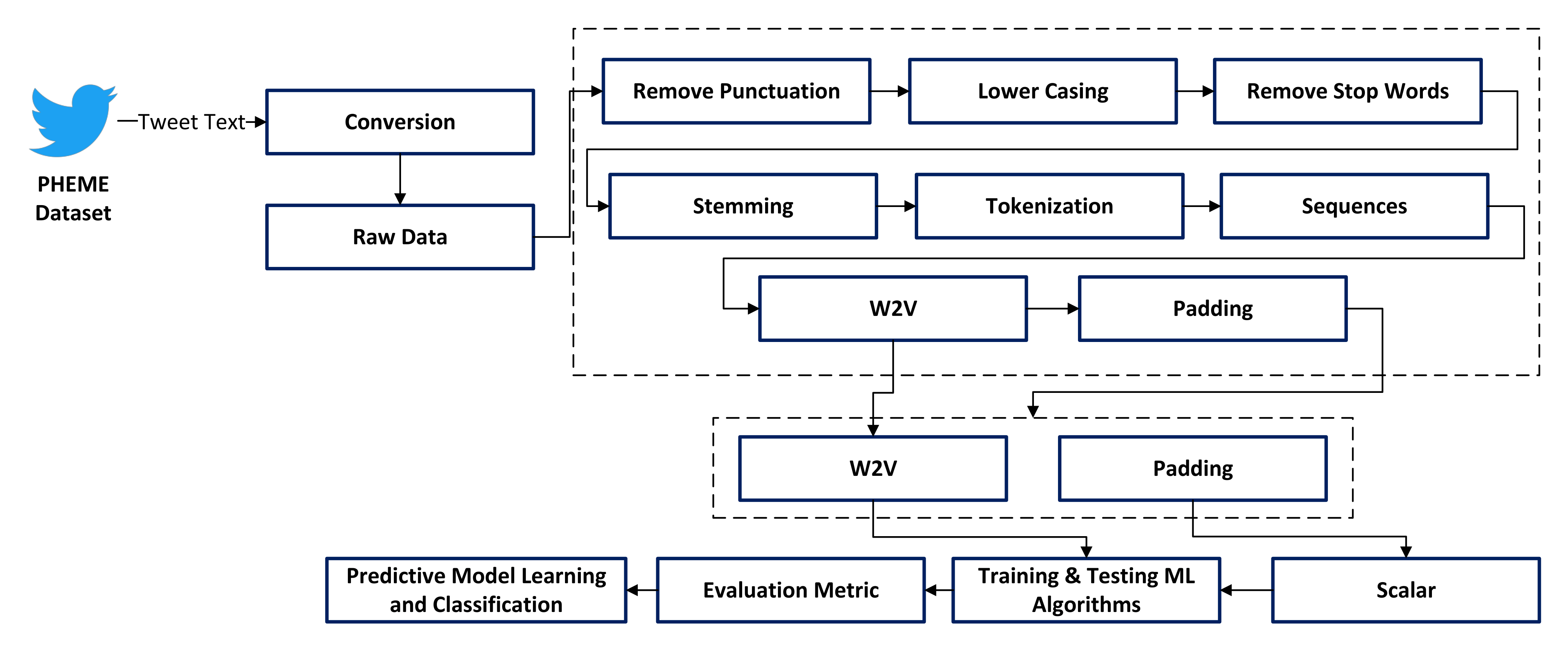
The text of tweets was obtained from the PHEME data set in our suggested model. The PHEME data set is open to the public. The PHEME data set is in JSON format, which needs to be converted to a csv file before preprocessing. We discuss each function in the section during preprocessing. After preprocessing, we feed the data to the word2vec model as shown in Figure 2. The word2vec model converts text data into vector form and applies padding to the output of word2vec. After that, we apply a standard scalar to the padding output and divide the data into train–test halves. As evaluation metrics, we use precision, recall, and F1, and then transfer that information to a machine learning model for rumor prediction.
4.1. Data Set
Data sets may differ depending on the platforms from which the data were obtained, the types of content contained, and whether or not propagation information was recorded, among other factors. The data sets for rumor detection are listed in Table 1. Five sets of real-life PHEME tweets were used in this study [26]. The PHEME dataset is the public dataset. The PHEME dataset was used in [10]. The dataset was collected from twitter by crawling different tweets using the twitter API. This dataset consists of rumors and non-rumors collected from twitter during breaking news. The detailed description of the five datasets is as follows. All events related to the PHEME dataset and the total number of rumors and non-rumors are shown in the Table 1.
The structure of the dataset is as follows. Each event has a directory with two subfolders, i.e., rumor and non-rumor. These two folders have the folder name with the tweet Id. The original tweet can be found on the folder that is named “source tweet,” and the reaction directory contains all reaction tweets. This dataset is a labeled dataset. One represents rumor, and zero represents non-rumor. The cleaning process of data is applied in two different steps. The first step is to remove the null value, and the second is to remove the deactivated ID.
4.2. Pre Processing
The pre-processing step is the foundation of every project’s whole execution phase. Cleaning, pre-processing, and outlier elimination are all part of this step. The data were extracted from the tar extension using Winrar programmed after it was downloaded. RStudio4 was used to understand and pre-process the data after they were extracted. For further processing, the data were transformed from JSON to a data frame. The data were made up of numerous JSON files, including all of the information from a single tweet. The username, location, text of the tweet, date, and time were all included in the data. For each event, this phase was performed for both rumors and non-rumors. We erased data from deactivated Ids during data preparation. Additionally, empty cells should be removed from the dataset. Sentiment analysis was used to preprocess tweet text data. It is the process of recognizing and categorizing opinions from a piece of text, whether the reaction tweet is good, negative, or neutral to the original tweet. It evaluates each word in a sentence to determine the sentence’s overall polarity. In the preprocessing step, remove the special character, remove punctuation, remove stop words, and remove word stemming. Many machine learning models perform well on data with features that are similar in scale or closely linked to the normal distribution. We utilized standard scalar features for data normalization. We subtracted the mean and then scaled the unit difference in standard scalar, then divided the total value by the standard deviation to get the unit difference.
4.2.1. Feature Extraction
Word2Vec Embedding
Word embedding is one of the most prominent ways of representing document vocabulary. Word2vec detects a words in the context of the document, as well as lexical and synthetic matching and the relationship between other words. Word2vec is a commonly used neural network model for acquiring word embedding using text as an input of word2vec and obtains a vector with low dimensionality of the words that appear in the text corpus. In our approach, word2vec transforms text data into vectors, which are then placed into a deep learning network for rumor prediction. The representation of a vector is called word embedding. Here, we consider as a sentence in the text and the surrounding of is the set of words within a window size that is specified. Skip-gram trains the representation of words of each word and its context words in order to build the vector space model. The objective is to discover meaningful representations of these phrases in the input matrix so that the model can predict the surrounding context words with strong possibility and another one with low probability, given any other word . The main objective of the skip-gram model is to maximize the log probability of the model, given a series of words ,, … and the surrounding window of size z:
Base Line Features
The baseline features used in existing studies are shown in Table 2.
Proposed Features
In this section, social-based and content-based proposed features are described, using a significant way of feature selection known as the correlation-based feature selection method. All the proposed features are described below. The following subsections briefly define all sort of characteristics to be used in this research.
Readability of Tweet
The readability of a tweet is a number that tells us how easy it will be for someone to read a particular piece of text. The grammatical readability score is based on the average length of the sentences and words.
Cosine Similarity between Source and Reaction
Cosine similarity is a metric used to determine the similarity of document, irrespective of their size. In this research, we measure the cosine similarity between the source tweet and reaction tweet: how the tweets are similar to each other.
Negative Sentiment in Reaction Tweet
The word sentimentality mostly refers to the appropriate polarity of a text or document, denoting the emotional outcome that the text or document has on the reader. It also specifies the attitude of the user about the topic. Negative sentiment refers to the inclusion of chances of reporting, hiding, blocking a post, etc.
Positive Sentiment in Reaction Tweet
Positive sentiment includes all consumption, such as likes, comments, shares, etc.
Neutral Sentiment in Reaction Tweet
Neutral sentiment includes a click or a scroll but has no follow through for consumption, i.e., someone just checked out the image.
Ratio of Positive Tweet
On Twitter, the ratio of positive tweets means that the total number of replies of a tweet significantly outperforms the total number of likes of that tweet.
Ratio of Negative Tweet
On twitter, a ratio occurs when the amount of responses to a tweet considerably outperforms the number of likes of a retweet. This demonstrates that individuals will dislike a tweet but not engage in its content.
User Verified
As to whether the current user account is verified or non-verified, 1 represents a verified account and 0 represents a non-verified account.
Total Number of Verified Followers
How many verified followers of users.
Overall Tweet Polarity
The popularity of a tweet is defined as the total sum of retweets, and the number of replies is divided by the total number of user followers, which is then multiplied by 100 by the proven fan interest percentage that is interacting with the tweets. We propose Tweet popularity as the following equation:
Specific Term
“Are you sure”, “Is it true”,” Fake?” etc. These terms are used in particular tweets: 1 represents the availability of these terms used in a tweet, and 0 represents that these terms are not used in a tweet.
Frequency of Specific Term
It represents the total number of these terms used in a reaction tweet.
Rank of User Attention
When the user catches a lot of consideration, it can be determined that the user is more responsible or responsible. The ratio of competitors to followers of a user replicates the gratitude of the user’s message. It is defined as
where i is the total number of the i-th tweet; comment means the total number of comments on the i-th tweet; retweet means the total number of forwarding messages of the i-th tweet; and follower means the total number of user followers.
4.3. Machine Learning for Rumor Detection
4.3.1. Data Mining Classifier
Support Vector Machine
The Support Vector Machine (SVM), which is available in numerous kernel functions, is another architecture for binary classification issues. The main objective of SVM in this research is generating a hyper plane based on features set for data points classification [27,28]. In this research, our main objective is to find the best hyper plan that classifies the data point with the greatest margin. Ref. [29] explains the mathematical concept of the cost function for the SVM model.
such that
A very well-known supervised machine learning model for classification is SVM. It has a reputation for being extremely accurate while consuming very little computing power. It is based on the hyper plane principle. This approach separates the data into distinct classes by inserting hyper planes in N-dimensional space. The results are stated in Section 5.1.1.
Random Forest
Random forest is an enhanced version of decision tree that is used for supervised learning. Random forest is characterized by a significant number of decision trees that are used to predict the target class. This prediction criterion is based on the highest number of votes. When we compare the random forest with other classifiers, its error rate is low due to the lack of proper connection between trees [30]. In this research, we train our random forest model by using different parameters, i.e., different number of predictions that are used in the search algorithm to obtain the optimal solution or model that can predict the outcome values accurately. We use the Gini index as a cost function to estimate a split in the dataset for the classification task. The Gini index is determined by subtracting one from the total squared probability of each class.
Random forest can be thought of as a collection of trees that work together as an ensemble model. This classifier creates a number of decisions trees and then uses a majority vote to determine the final prediction. This is more effective than decision trees since the decision trees work together as a group and correct each other’s mistakes. Each tree in a random forest is trained using different bits of data and features bagging. As a result, the trees are unrelated to one another.
Logistic Regression
A logistic regression algorithm is used to classify the text into a binary class that deals with large number of features because it provides a straightforward equation for classifying problems into a binary class [31]. To obtain the best outcome for all datasets, we use these equations and perform a hyper parameter adjustment. The logistic regression hypothesis function is a mathematical function that calculates the probability of a certain event occurring. By using a sigmoid function, the output value of logistic regression is transformed into a probability value. The cost function is computed as follows:
Gaussian Naive Bayes
Gaussian naive Bayes is a more advanced version of naive Bayes. All variables in naive Bayes must be categorical. However, the data used in this study include numeric data. As a result, Gaussian naive Bayes is used, which assumes that the data are Gaussian. This classifier is also chosen since naive Bayes is often regarded as one of the most effective classifier models. This classifier employs the partial t technique, which is advantageous in large datasets because it takes chunks of data into account when training the classifier.
4.3.2. Neural Network for Rumor Detection
Neural networks are used in deep learning algorithms to learn about data and classify them. In a typical neural network, each weight has a connection that transforms it and creates a neuron’s input. The sigmoid activation function is used in this project, which has two layers. No other research effort has ever taken this method. This is used to determine if neural networks or supervised learning models perform better.
Recurrent Neural Network
A recurrent neural network consists of a network that uses recurrent connections to access memory. In a feed forward recurrent neural network, inputs are independent of one another; however, in an RNN, all inputs are reliant on or related to one another. The structure of RNN is shown in Figure 3.
Before discussing the RNN, we discuss the feed forward neural network. In a feed forward neural network, there is no memory space for storing the previous state results, which is why a feed forward neural network cannot manage the time series problem. In recurrent neural network, RNN, there is a memory unit that stores the result of previous states as well as that of the current state. The method of RNN is shown in Figure 3. From Equation (10), is the current state, is the previous state, and is the current input state. In RNN, we consider the current input state as well as the previous state at the above given equation. This function returns the current state RNN performance function on each input state. In Equation (11), a tanh activation function is used. In Equation (11), is the current input, is the weight of the previous hidden state, and is the weight of the current input state. Equation (12) show the output results of RNN: in the output state, the weight of the output state is shown.
In Equation (10), is the current state, is the previous state of RNN, and represents the current state. In RNN, we use the current input with the previous output state, and f represents some function.
In Equation (11), tanh is the activation function, is the weight of the previous hidden state, and is the weight of the current hidden state.
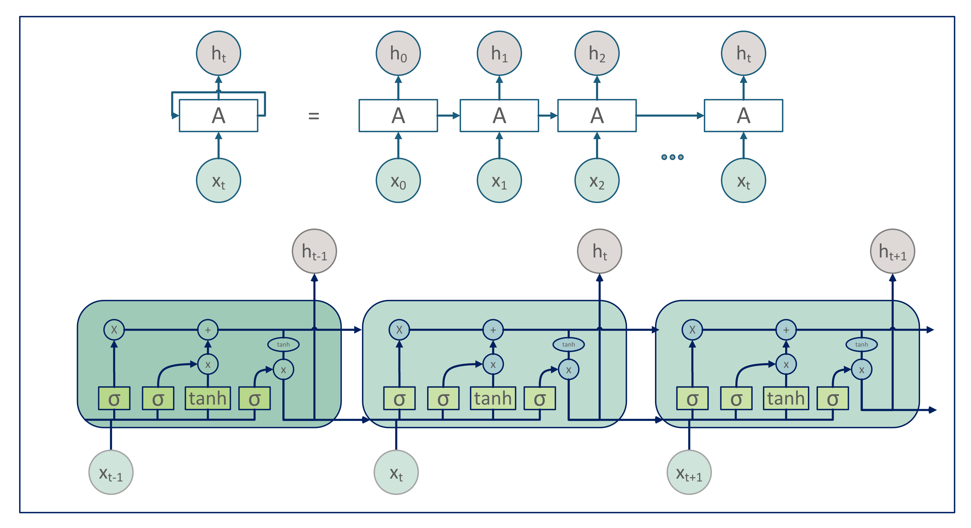
Long Short-Term Memory
Recurrent neural networks are a type of network that uses recurrent connections to build memory. The notes they receive trigger RNN notes. On the other hand, the LSTM gate accepts or rejects the data based on their weight. Later, these signals become disturbed by their own weight. The RNN learning process then adjusts the weights that regulate the hidden state and input. However, these calls learn when they obtain some information, output some information or delete information through the consequential steps of taking back propagation error. An LSTM unit, unlike a standard recurrent unit (Equations (13)–(18)), preserves a memory cell at time t. The following formulas are used to calculate an LSTM unit’s output ht.
A logistic sigmoid function is defined as follows: the amount of new memory added to the memory cell is controlled by the input gate. The extent to which the present memory is lost is determined by the forget gate . The memory is updated by forgetting part of the old memory and inserting new memory . represent the output gate of a memory as shown in Figure 4.
Bidirectional Long Short-Term Memory
The flow of bidirectional LSTM is not just backward to forward but also forward to backward, using two hidden layers. As a result, Bi-LSTMs have a better understanding of the situation. Bi-LSTMs were optimized to enhance the amount of input data that the network could utilize [16]. Bi-RNN is a process that involves breaking the neurons of a traditional RNN into bidirectional connections. The one is for the backward state direction, while the other is for the forward state direction. The model equation is used to update the network’s hidden layer and generate the outputs.
where symbol is used for the logistic sigmoid function, the input, forget output gates, which are and c, and the cell input activation vector, respectively. In bidirectional LSTM RNN, we set the value of the maximum sequence length as 50, and the number of embedding dimension as 300, setting the input length as the same as the maximum sequence length. The dropout rate is 0.2, and we use the sigmoid activation function. The batch size is 34. The total number of epochs is 10, and the loss function is set to binary cross-entropy. For choosing an optimizer, we use ‘Adam because it performs well as compared to Soft-Max.
Recurrent neural network is a sequential model. In natural language, the processing order of words is very important to the meaning. In our research of tweets, the word order is important. RNN have been widely used for a variety of applications, including text classification and sequence generation. A typical RNN works as follows. Given an input vector sequence x of length T, denoted by , for each time step t = 1 to T, the algorithm iterates over the following equations to update the hidden states of the network, , and generate the outputs, . The main objective of backpropagation is to minimize the error and improve the prediction result.
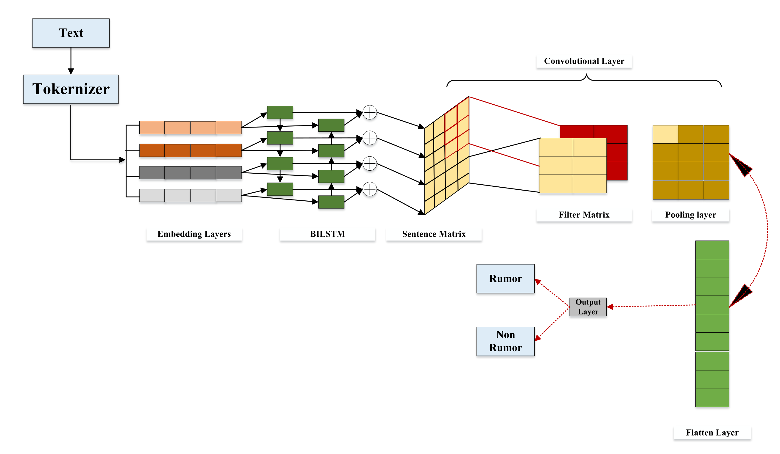
In Figure 5, we obtain the tweet text and pass it to the tokenizer. Tokenization is a technique that is used to break down a large text message or phrase into smaller pieces. In the NLP model, tokenization helps to understand the context of words. The embedding layer is the first hidden layer of a network. This hidden layer must have the following hidden argument: the total number of words in the text data. For the activation function, softmax function is used to predict the probability distribution of the neural network. To reduce dimensionality, pooling is typically used after a convolution procedure. By restricting the number of factors, this saves time while also decreasing overfitting. The most frequent sort of pooling is max pooling, which simply takes the pooling window’s maximum value. Flattening is the process of converting data into one-dimensional arrays. To construct a single continuous feature vector, we convert the output of the convolutional layers. It is also connected to the fully connected layer. In the output layer, we obtain our model’s final prediction outcome, which is either a rumor or not a rumor.
4.4. Evaluation Metrics
The following performance metrics are utilized.
4.4.1. Precision
The percentage of true positive instances predicted to be positive.
4.4.2. Recall
Proportion of true positive instances from cases that are actually positive.
4.4.3. F-Measure
It is the mean of the precision and recall.
5. Experimental Results
5.1. Rumor Detection Results and Comparisons
Precision, recall, and F1 measurements are utilized to assess the performance of the proposed features in comparison to the current baseline characteristics [10]. These are conjoint evaluation metrics used for evaluating any classification problem. The experimental setup and hardware requirements are listed in Table 3. To assess the performance of a classification method, experiments are carried out using 5-fold cross validation.in this research use four datasets to train our data and the baseline classifier, and fifth dataset to assess the performance of these classifiers using precision, recall, and the F1 measure. As a consequence of evaluating all five runs of the dataset, the evaluation result indicates undetected topic rumors. Each 5-fold run should be repeated five times for each model. They identify the rumor and non-rumor ranges from 0 to 1. Therefore, the design of the research is a binary classification problem. We use sci-kit-learn library [32] for the classification problem.
5.1.1. Results
We used a 5-fold cross validation technique with the suggested model to validate the findings shown in Table 4. The calculated results are the micro-averaged precision, recall, and F1 scores throughout all five runs for both rumors and non-rumors. The given values for our proposed model are the micro-averaged variance scores across five 5-fold cross-validation repetitions. When the overall performance of SVM, random forest, naive Bayes, and logistic regression were evaluated, it was clear that random forest (RF) exceeded in terms of precision and F1 as shown in Table 4. The foundation of SVM is the support vectors and hyper planes. One of the most often used classification methods is the SVM method. With the baseline classifier, the output of this algorithm is depicted in Figure 6 where it can be seen that SVM performs best in terms with precision 0.41, recall 0.53, and F1 0.44. Figure 6a,c shows the overall performance of proposed outcomes when compared to non-rumors results. Our SVM performs best in terms of precision and recall. The baseline SVM precision results are 0.67, recall is 0.56, and F1 is 0.61. However, our recommended results are 0.69 precision and with 0.63 F1. We performed a 5-fold cross validation and received the same findings as in Figure 6 with the suggested model and the baseline classifiers. The reported values are the micro-averaged precision, recall, and F1 scores for both rumors and non-rumors throughout all five runs. The presented values for our proposed model are the micro-averaged variance scores across five 5-fold cross-validation repetitions. When we compare the overall performance of SVM, RF, NB and LR, it can be seen that in Table 4 logistic regression (LR) outperformed all baseline classifiers in terms of precision and F1, at 0.66 and 0.59, respectively. However, when we compared these four algorithms with the non-rumor table shown, it could be seen that, overall, naïve Bayes had the best performance in terms of precision, and random forest had the best performance in terms of recall and F1 at 0.81, 0.76, and 0.78 shown in Table 4 and Table 5, respectively. SVM is built on the foundations of support vectors and hyper planes. The SVM method is one of the most extensively used classification algorithms. The output of this algorithm is shown in Table 2. When comparing the results with the baseline classifier, it can be noted that SVM performs best in terms of precision 0.41, recall 0.53, and F1 0.44. While comparing the results with non rumors, Figure 6 shows both rumor and non-rumor results of the baseline and our proposed model. Our SVM performs best in terms of precision and recall. The baseline SVM precision results are 0.67, recall is 0.56, and F1 is 0.61. However, our recommended results are 0.69 precision; with 0.66, Naive Bayes has the best performance in term of recall. Figure 6 shows the baseline and predicted results in both classes, rumor and non rumor, by using precision, recall and F1. They are the micro-average results of precision, recall and F1 on 50 epochs.
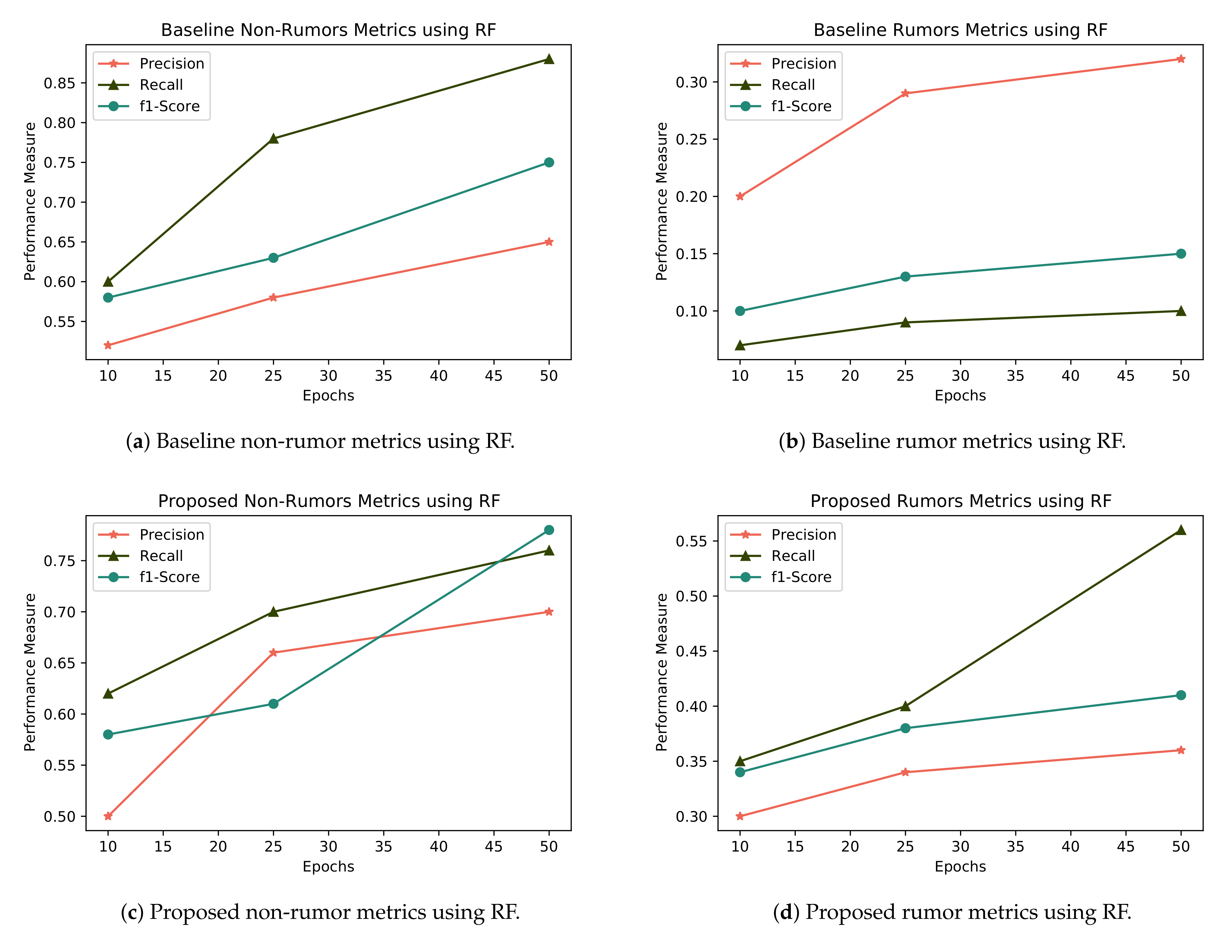
We compare the results of random forest with baseline algorithms results in term of rumor and non rumor detection, shown in Table 4 and Table 5, respectively. The calculated results are also shown in Figure 7. Our proposed features perform best in terms of precision, recall and F1, at 0.36, 0.756 and 0.41, respectively. While comparing with non-rumors, random forest performs best in term of precision and F1.
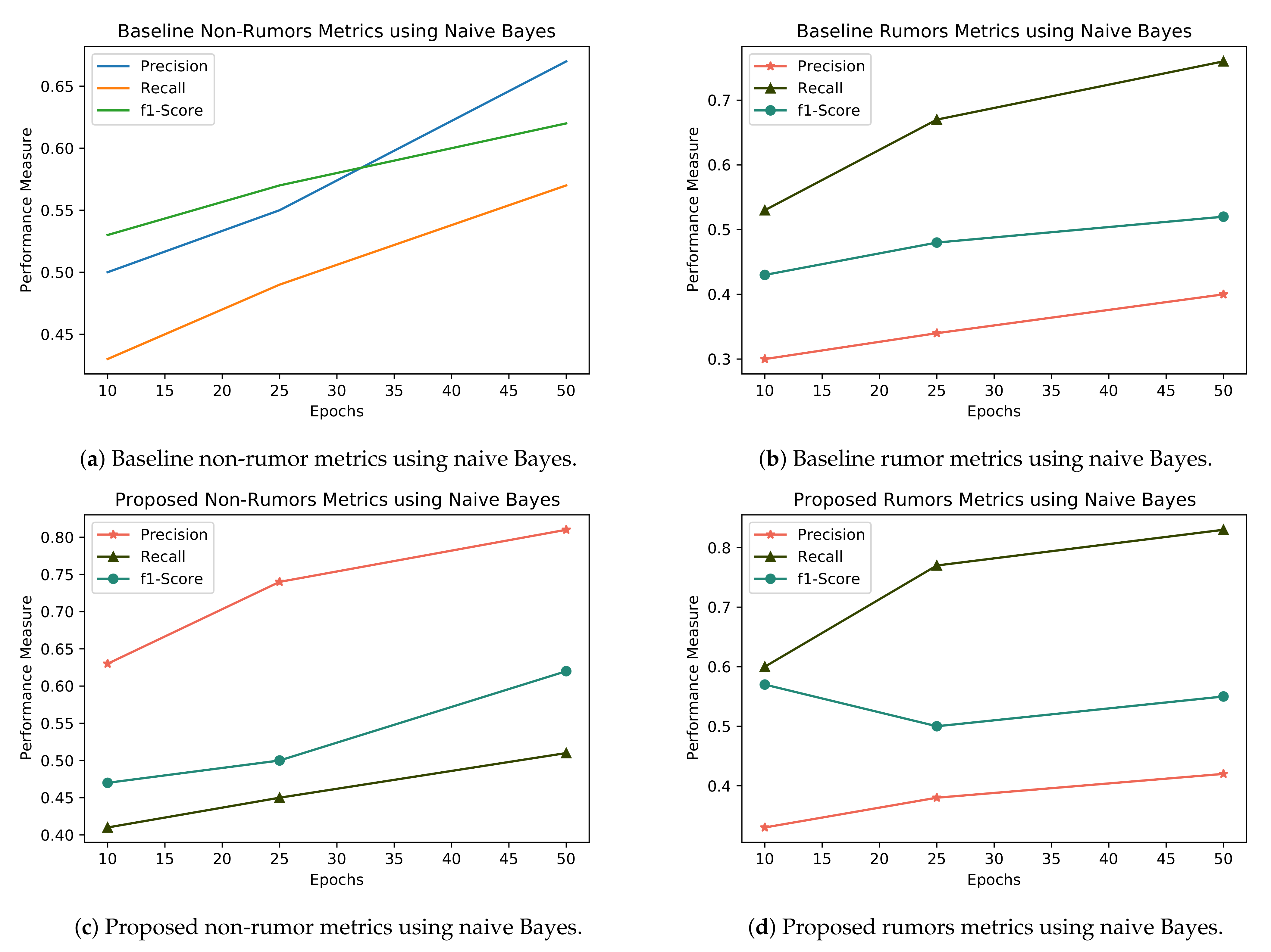
Now, we compare the results of naïve Bayes with the baseline classifier in term of rumors that are shown in Table 4. Our proposed features perform best using naive Bayes in terms of precision recall and F1 that are 0.42, 0.83 and 0.55, respectively, as shown in Figure 8. However, when we compare the results of naïve Bayes with the non-rumor results that are shown in Table 5, our proposed features perform best when we compare the state-of-the-art baseline features in term of precision, recall and F1. Similarly, logistic regression outperforms both classes of rumors and non-rumors as shown in Table 4 and Table 5.
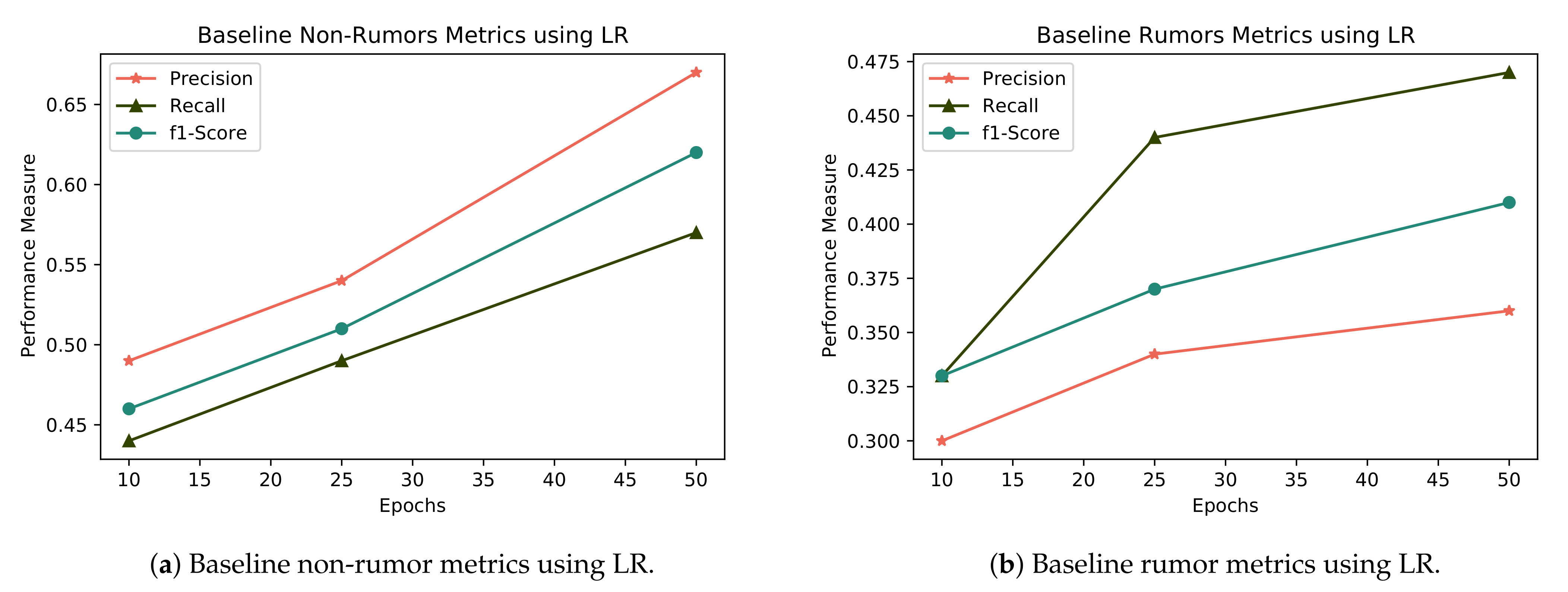
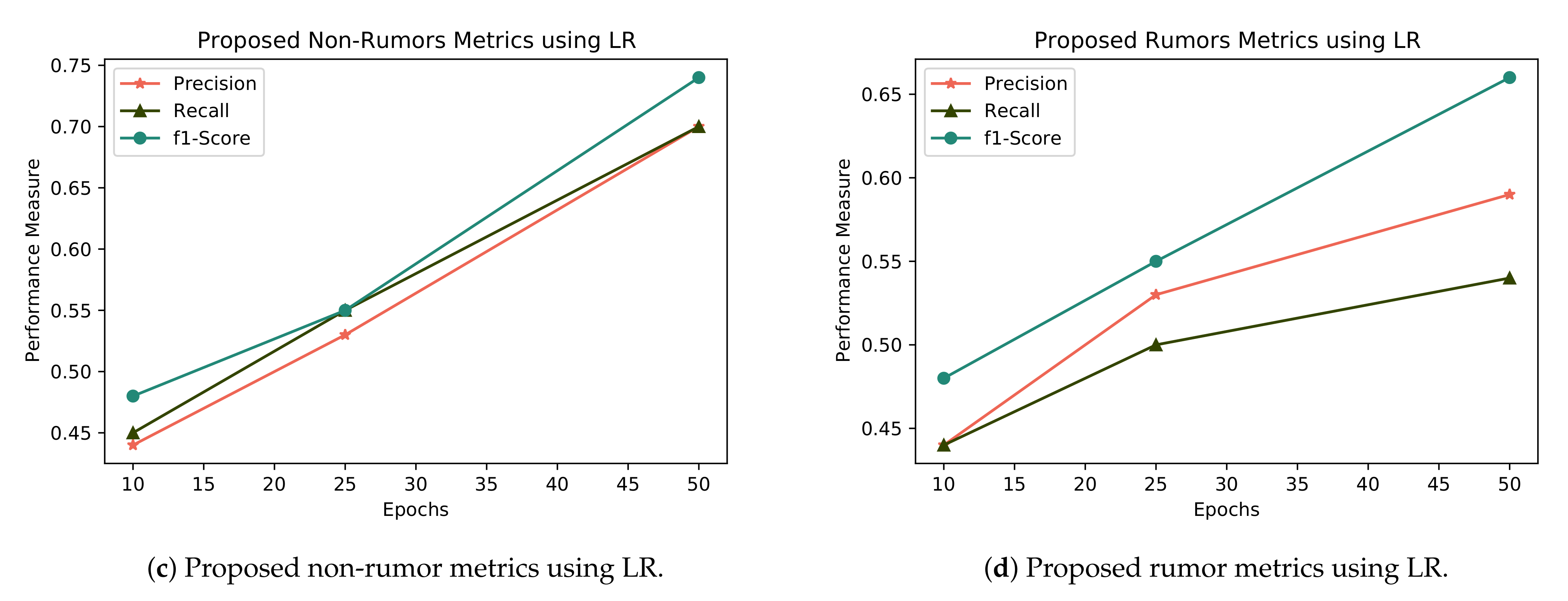
When we compare the results of logistic regression with the state-of-the-art baseline classifier in term of rumors and non rumors, Figure 9 shows that our proposed features with the baseline model perform best in overall precision, recall and F1, while, when comparing with the non-rumor class, logistic regression also performs best in precision, recall and F1, which are 0.70, 0.70, and 0.74, respectively.
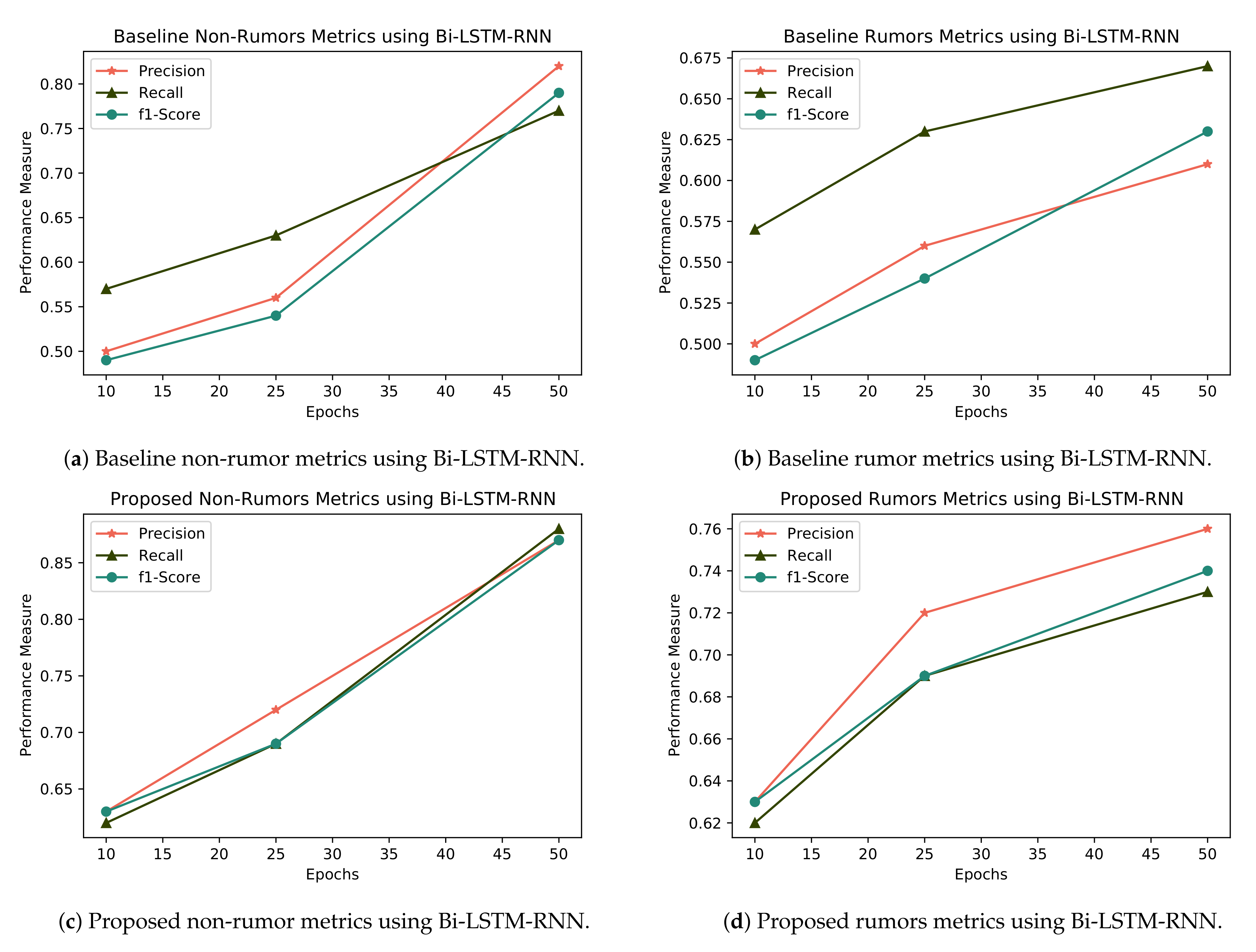
Now, we apply our proposed deep learning model on the same dataset. It produces best results overall for both classes of rumor and non rumor, compared with the state-of-the-art baseline classifier in terms of precision, recall and F1 as shown in Figure 10. These computed results shows that our model and new proposed features perform best when comparing all baseline classifiers, in detecting rumors and non-rumors by using only the text data of a tweet without content and social-based features as shown also in Table 4 and Table 5. Bi-LSTM is the most widely used categorization approach. In this algorithm, we apply deep learning mode on text data. The results of this approach are shown in Figure 10. When compared to the baseline classifier, our suggested Bi-LSTM RNN has a precision of 0.77, a recall of 0.73, and an F1 of 0.74. When comparing the non-rumor findings to the baseline classifier, as seen in Table 3, Bi-LSTM-RNN performs best in terms of precision and recall. In the baseline LSTM RNN, precision is 0.82, recall is 0.77, and F1 is 0.79; however we recommend 0.87 precision, 0.88 recall, and 0.87 F1 score.
Table 6 shows the average precision score of different classifiers using only content-based features and after using hybrid content and social-based features to measure the impact of social-based features. On the Ferguson dataset, when applying naïve Bayes on only content-based features, the average precision score is 0.64, and after this, both social- and content-based features were merged and naïve Bayes was applied, increasing the result by 0.2. In some classifiers, they have much importance for social-based features, and some classifiers have no positive impact on social-based features.
6. Conclusions
With the rising use of social media as a primary source of breaking news, separating verifiable information from unsubstantiated rumors has become a challenging and critical undertaking. Several features of social media make it easier to post material with unknown truth values and for that information to spread quickly among users all over the world. If not identified as soon as feasible, breaking-news rumors might have disastrous implications. Most of the existing work on rumor identification from social media relies on manually extracting features or rules. In this study, we offer a novel set of features for rumor identification in Twitter by using a deep learning framework. Using the change of aggregated information over multiple time intervals associated with each event, our technique learns Bi-LSTM RNN models. We compare our Bi-LSTM RNN-based technique to baseline LSTM-RNN frequently used recurrent units, tanh, and LSTM, and find that our model outperforms the state-of-the-art methods. In Bi-LSTM RNN, we add many hidden layers and embedding layers for even more improvement. In addition, we calculate a new set of characteristics and compare our results to the best-in-class baseline result. The technique can yet be improved. In the future, more rigorous tests will be required to better understand how deep learning aids rumor detection. Due to a large amount of unlabeled data available on social media, we may also construct unsupervised models.
Author Contributions
Conceptualization, T.A., A.R., P.W.K. and M.S.F.; methodology, T.A., A.M., M.S.F. and R.A.; software, T.A., M.S.F., R.A. and A.M.; validation, M.S.F., R.A. and A.R.; Formal Analysis, T.A. and M.S.F.; investigation, R.A. and M.S.F.; data curation, A.R., P.W.K. and A.M.; writing—original draft preparation, T.A., A.R. and P.W.K.; writing—review and editing, M.S.F., R.A. and A.M.; visualization, A.R. and T.A.; supervision, M.S.F. and R.A.; project administration, R.A.; funding acquisition, R.A. and M.S.F. All authors have read and agreed to the published version of the manuscript.
Funding
Princess Nourah bint Abdulrahman University Researchers Supporting Project number (PNURSP2022R323), Princess Nourah bint Abdulrahman University, Riyadh, Saudi Arabia.
Acknowledgments
The authors express their gratitude to Princess Nourah bint Abdulrahman University Researchers Supporting Project number (PNURSP2022R323), Princess Nourah bint Abdulrahman University, Riyadh, Saudi Arabia.
Conflicts of Interest
The authors declare no conflict of interest.
References
- Matsa, K.E.; Shearer, E. News Use Across Social Media Platforms 2018; Pew Research Center: Washington, DC, USA, 2018; Volume 10. [Google Scholar]
- Incredible and Interesting Twitter Stats and Statistics. Available online: https://www.brandwatch.com/blog/twitter-stats-and-statistics/ (accessed on 12 August 2021).
- Domm, P. False rumor of explosion at White House causes stocks to briefly plunge; AP confirms its Twitter feed was hacked, CNBC. COM 2013, 23, 2062. [Google Scholar]
- Glaser, S.; Dutt, M.; MacArthur, J.; Sorenson, A. Supporting Online Material. Phys. Rev. Lett 2009, 102, 210502. [Google Scholar]
- Hermida, A. Twittering the news: The emergence of ambient journalism. J. Pract. 2010, 4, 297–308. [Google Scholar] [CrossRef]
- Castillo, C.; Mendoza, M.; Poblete, B. Predicting information credibility in time-sensitive social media. Internet Res. 2013, 23, 560–588. [Google Scholar] [CrossRef] [Green Version]
- Lies, Damn Lies and Viral Content 2015. Available online: https://academiccommons.columbia.edu/doi/10.7916/D8Q81RHH (accessed on 25 August 2021).
- Cai, G.; Wu, H.; Lv, R. Rumors detection in chinese via crowd responses. In Proceedings of the 2014 IEEE/ACM International Conference on Advances in Social Networks Analysis and Mining (ASONAM 2014), Beijing, China, 17–20 August 2014; pp. 912–917. [Google Scholar]
- Lee, L.F.; Hutton, A.P.; Shu, S. The role of social media in the capital market: Evidence from consumer product recalls. J. Account. Res. 2015, 53, 367–404. [Google Scholar] [CrossRef]
- Alkhodair, S.A.; Ding, S.H.; Fung, B.C.; Liu, J. Detecting breaking news rumors of emerging topics in social media. Inf. Process. Manag. 2020, 57, 102018. [Google Scholar] [CrossRef]
- Qazvinian, V.; Rosengren, E.; Radev, D.; Mei, Q. Rumor has it: Identifying misinformation in microblogs. In Proceedings of the 2011 Conference on Empirical Methods in Natural Language Processing, Scotland, UK, 27–31 July 2011; pp. 1589–1599. [Google Scholar]
- Takahashi, T.; Igata, N. Rumor detection on twitter. In Proceedings of the 6th International Conference on Soft Computing and Intelligent Systems, and the 13th International Symposium on Advanced Intelligence Systems, Kobe, Japan, 20–24 November 2012; pp. 452–457. [Google Scholar]
- Wang, D.; Irani, D.; Pu, C. A social-spam detection framework. In Proceedings of the 8th Annual Collaboration, Electronic Messaging, Anti-Abuse and Spam Conference, Perth, Australia, 1–2 September 2011; pp. 46–54. [Google Scholar]
- Zhang, Q.; Zhang, S.; Dong, J.; Xiong, J.; Cheng, X. Automatic detection of rumor on social network. In Natural Language Processing and Chinese Computing; Springer: Berlin/Heidelberg, Germany, 2015; pp. 113–122. [Google Scholar]
- Hamidian, S.; Diab, M. Rumor identification and belief investigation on twitter. In Proceedings of the 7th Workshop on cOmputational Approaches to Subjectivity, Sentiment and sOcial Media Analysis, San Diego, CA, USA, 16 June 2016; pp. 3–8. [Google Scholar]
- Thakur, H.K.; Gupta, A.; Bhardwaj, A.; Verma, D. Rumor detection on Twitter using a supervised machine learning framework. Int. J. Inf. Retr. Res. 2018, 8, 1–13. [Google Scholar] [CrossRef]
- Geng, Y.; Sui, J.; Zhu, Q. Rumor detection of Sina Weibo based on SDSMOTE and feature selection. In Proceedings of the 2019 IEEE 4th International Conference on Cloud Computing and Big Data Analysis (ICCCBDA), Chengdu, China, 12–15 April 2019; pp. 120–125. [Google Scholar]
- Sicilia, R.; Giudice, S.L.; Pei, Y.; Pechenizkiy, M.; Soda, P. Twitter rumour detection in the health domain. Expert Syst. Appl. 2018, 110, 33–40. [Google Scholar] [CrossRef]
- Liu, Y.; Jin, X.; Shen, H. Towards early identification of online rumors based on long short-term memory networks. Inf. Process. Manag. 2019, 56, 1457–1467. [Google Scholar] [CrossRef]
- Riquelme, F.; González-Cantergiani, P. Measuring user influence on Twitter: A survey. Inf. Process. Manag. 2016, 52, 949–975. [Google Scholar] [CrossRef] [Green Version]
- Ma, J.; Gao, W.; Mitra, P.; Kwon, S.; Jansen, B.J.; Wong, K.F.; Cha, M. Detecting Rumors from Microblogs with Recurrent Neural Networks. In Proceedings of the 25th International Joint Conference on Artificial Intelligence (IJCAI 2016), New York, NY, USA, 9–15 July 2016. [Google Scholar]
- Laylavi, F.; Rajabifard, A.; Kalantari, M. Event relatedness assessment of Twitter messages for emergency response. Inf. Process. Manag. 2017, 53, 266–280. [Google Scholar] [CrossRef]
- Allport, F.H.; Lepkin, M. Wartime rumors of waste and special privilege: Why some people believe them. J. Abnorm. Soc. Psychol. 1945, 40, 3. [Google Scholar] [CrossRef]
- Ratkiewicz, J.; Conover, M.; Meiss, M.; Gonçalves, B.; Flammini, A.; Menczer, F. Detecting and tracking political abuse in social media. In Proceedings of the International AAAI Conference on Web and Social Media, Barcelona, Spain, 17–21 July 2011; Volume 5. [Google Scholar]
- Treadway, M.; McCloskey, M. Effects of racial stereotypes on eyewitness performance: Implications of the real and the rumoured Allport and Postman studies. Appl. Cogn. Psychol. 1989, 3, 53–63. [Google Scholar] [CrossRef]
- PHEME dataset for Rumour Detection and Veracity Classification. Available online: https://figshare.com/articles/dataset/PHEME_dataset_for_Rumour_Detection_and_Veracity_Classification/6392078 (accessed on 2 August 2021).
- Cristianini, N.; Shawe-Taylor, J. An Introduction to Support Vector Machines and Other Kernel-Based Learning Methods; Cambridge University Press: Cambridge, MA, USA, 2000. [Google Scholar]
- Rizwan, A.; Iqbal, N.; Ahmad, R.; Kim, D.H. WR-SVM model based on the margin radius approach for solving the minimum enclosing ball problem in support vector machine classification. Appl. Sci. 2021, 11, 4657. [Google Scholar] [CrossRef]
- Wang, L. Support Vector Machines: Theory and Applications; Springer Science & Business Media: Berlin/Heidelberg, Germany, 2005; Volume 177. [Google Scholar]
- Gregorutti, B.; Michel, B.; Saint-Pierre, P. Correlation and variable importance in random forests. Stat. Comput. 2017, 27, 659–678. [Google Scholar] [CrossRef] [Green Version]
- Mitchell, T.M. The Discipline of Machine Learning; Carnegie Mellon University, School of Computer Science, Machine Learning: Pittsburgh, PA, USA, 2006; Volume 9. [Google Scholar]
- Scikit-Learn: Machine Learning in Python—Scikit-Learn 1.0.1 Documentation. Available online: https://scikit-learn.org/stable/ (accessed on 7 August 2021).
Figure 1.
Annual twitter users.

Figure 2.
Proposed block model.

Figure 3.
Architecture of RNN.

Figure 4.
Architecture of LSTM.

Figure 5.
Proposed rumor detection model.

Figure 6.
SVM for rumor and non-rumor detection with baseline and proposed features.

Figure 7.
RF for rumor and non-rumor detection with baseline and proposed features.

Figure 8.
Naive Bayes for rumor and non-rumor detection with proposed features.

Figure 9.
LR for rumor and non-rumor detection with baseline and proposed features.


Figure 10.
Proposed Bi-LSTM-RNNfor rumor and non-rumor detection with baseline and proposed features.
Figure 10.
Proposed Bi-LSTM-RNNfor rumor and non-rumor detection with baseline and proposed features.


Table 1.
Dataset details.
| Dataset | Rumor | Non-Rumor | Total |
|---|---|---|---|
| Charlie Hebdo | 458 | 1621 | 2079 |
| Ferguson | 284 | 859 | 1143 |
| Germanwings Crash | 238 | 231 | 469 |
| Ottawa Shooting | 470 | 420 | 890 |
| Sydney Siege | 522 | 699 | 1221 |
Table 2.
Baseline features.
| Social Based | Content Based |
|---|---|
| # Tweets | Words Vector |
| # Lists | Total Number of Capital ratio |
| Follow Ratio | # Question mark |
| Age | # Exclamation mark |
Table 3.
Hardware and software requirements.
| Sr No. | Component | Description |
|---|---|---|
| 1 | Hardware | Intel Core i5 6th Gen PC |
| 2 | Operating System | Window 10 |
| 3 | Memory | 8 GB RAM |
| 4 | Server | SQL Server |
| 5 | Libraries | Pandas, Sklearn, spaCy, TextBlob |
| 6 | Storage | MS Excel |
| 7 | Core Programming language | Python |
| 8 | IDE | Anaconda Navigator(3) |
Table 4.
Comparison of Rumor Class Result with state of the art baseline.
| Classifier | Baseline Rumors Result | Proposed Rumor Result | ||||
|---|---|---|---|---|---|---|
| Precision | Recall | F-1 | Precision | Recall | F-1 | |
| SVM | 0.35 ± 0.45 | 0.45 ± 0.18 | 0.39 ± 0.84 | 0.41 ± 0.74 | 0.53 ± 0.39 | 0.44 ± 0.55 |
| Random Forest | 0.32 ± 0.72 | 0.10 ± 0.83 | 0.15 ± 0.71 | 0.36 ± 0.38 | 0.56 ± 0.91 | 0.41 ± 0.12 |
| Naïve Bayes | 0.40 ± 0.89 | 0.76 ± 0.19 | 0.52 ± 0.67 | 0.42 ± 0.38 | 0.83 ± 0.74 | 0.55 ± 0.62 |
| Logistic Regression | 0.36 ± 0.12 | 0.47 ± 0.92 | 0.41 ± 0.61 | 0.66 ± 0.34 | 0.54 ± 0.27 | 0.59 ± 0.24 |
| Bi-LSTM-RNN (Text) | 0.61 ± 0.64 | 0.67 ± 0.39 | 0.63 ± 0.83 | 0.76 ± 0.14 | 0.73 ± 0.74 | 0.74 ± 0.63 |
Table 5.
Comparison of non-rumor class result with state-of-the-art baseline.
| Classifier | Baseline Non-Rumors Result | Proposed Non- Rumor Result | ||||
|---|---|---|---|---|---|---|
| Precision | Recall | F-1 | Precision | Recall | F-1 | |
| SVM | 0.67 ± 0.17 | 0.56 ± 0.65 | 0.61 ± 0.41 | 0.69 ± 0.38 | 0.55 ± 0.14 | 0.63 ± 0.38 |
| Random Forest | 0.65 ± 0.18 | 0.88 ± 0.96 | 0.75 ± 0.24 | 0.70 ± 0.45 | 0.76 ± 0.74 | 0.78 ± 0.69 |
| Naïve Bayes | 0.77 ± 0.52 | 0.41 ± 0.18 | 0.51 ± 0.36 | 0.81 ± 0.81 | 0.51 ± 0.94 | 0.62 ± 0.64 |
| Logistic Regression | 0.67 ± 0.84 | 0.57 ± 0.55 | 0.62 ± 0.17 | 0.70 ± 0.94 | 0.70 ± 0.31 | 0.74 ± 0.57 |
| Bi-LSTM-RNN (Text) | 0.82 ± 0.82 | 0.77 ± 0.65 | 0.79 ± 0.87 | 0.87 ± 0.18 | 0.88 ± 0.64 | 0.87 ± 0.24 |
Table 6.
Average precision scores of different classifiers before and after using social-based features associated with each dataset.
Table 6.
Average precision scores of different classifiers before and after using social-based features associated with each dataset.
| Dataset | NB | RF | SVM | CRF | LSTM-RNN | |||||
|---|---|---|---|---|---|---|---|---|---|---|
| Before | After | Before | After | Before | After | Before | After | Before | After | |
| Ferguson | 0.64 | 0.66 | 0.36 | 0.37 | 0.57 | 0.54 | 0.64 | 0.74 | 0.76 | 0.76 |
| Germanwings Crash | 0.65 | 0.63 | 0.76 | 0.21 | 0.51 | 0.53 | 0.62 | 0.64 | 0.65 | 0.54 |
| Ottawa Shooting | 0.65 | 0.72 | 0.48 | 0.62 | 0.58 | 0.56 | 0.70 | 0.69 | 0.61 | 0.54 |
| Sydney Siege | 0.71 | 0.69 | 0.49 | 0.57 | 0.51 | 0.49 | 0.71 | 0.72 | 0.66 | 0.60 |
| Charlie Hebdo | 0.59 | 0.60 | 0.56 | 0.47 | 0.49 | 0.45 | 0.81 | 0.84 | 0.75 | 0.75 |
Publisher’s Note: MDPI stays neutral with regard to jurisdictional claims in published maps and institutional affiliations. |
© 2022 by the authors. Licensee MDPI, Basel, Switzerland. This article is an open access article distributed under the terms and conditions of the Creative Commons Attribution (CC BY) license (https://creativecommons.org/licenses/by/4.0/).
Share and Cite
MDPI and ACS Style
Ahmad, T.; Faisal, M.S.; Rizwan, A.; Alkanhel, R.; Khan, P.W.; Muthanna, A. Efficient Fake News Detection Mechanism Using Enhanced Deep Learning Model. Appl. Sci. 2022, 12, 1743. https://0-doi-org.brum.beds.ac.uk/10.3390/app12031743
AMA Style
Ahmad T, Faisal MS, Rizwan A, Alkanhel R, Khan PW, Muthanna A. Efficient Fake News Detection Mechanism Using Enhanced Deep Learning Model. Applied Sciences. 2022; 12(3):1743. https://0-doi-org.brum.beds.ac.uk/10.3390/app12031743
Chicago/Turabian StyleAhmad, Tahir, Muhammad Shahzad Faisal, Atif Rizwan, Reem Alkanhel, Prince Waqas Khan, and Ammar Muthanna. 2022. "Efficient Fake News Detection Mechanism Using Enhanced Deep Learning Model" Applied Sciences 12, no. 3: 1743. https://0-doi-org.brum.beds.ac.uk/10.3390/app12031743
Note that from the first issue of 2016, this journal uses article numbers instead of page numbers. See further details here.