
Bridge Natural Frequencies, Numerical Solution versus Experiment

Department of Structural Mechanics and Applied Mathematics, Faculty of Civil Engineering, University of Zilina, 010 26 Zilina, Slovakia
*
Author to whom correspondence should be addressed.
Appl. Sci. 2022, 12(3), 1765; https://0-doi-org.brum.beds.ac.uk/10.3390/app12031765
Submission received: 14 January 2022
/
Revised: 1 February 2022
/
Accepted: 7 February 2022
/
Published: 8 February 2022
Abstract
:The article is dedicated to a numerical and experimental analysis of the basic natural frequencies of a bridge structure. It presents the results obtained using the finite element method and the frequency response functions applied in two variants, using the lumped mass model and the model with a continuously distributed mass, as well as the results obtained using the energy method. It describes a simple experiment to measure the response of a bridge to random excitations from rail traffic, and compares the values of selected natural frequencies obtained by numerical and experimental methods. It offers engineers alternative solutions for their applications in engineering practice. It tries to bring a complicated theory closer to engineering practice in the simplest possible way and, at the same time, arouses interest in its deeper study.
1. Introduction
The natural frequencies and natural modes unambiguously define the dynamic properties of the structure and, thus, describe its dynamic individuality. The knowledge of these characteristics is necessary for the analysis of the structure response to various dynamic loads. The dynamic response depends on the ratio between excitation and natural frequencies. The knowledge of natural frequencies makes it possible to predict the response at a known frequency composition of the load. For example, the bridge mentioned at the end of Chapter 5 oscillates with a dominant frequency corresponding to the first natural frequency when one vehicle is driven. When moving a continuous traffic flow, the dominant oscillation frequency corresponds to the second natural frequency. These characteristics can be obtained numerically or experimentally. The finite element method (FEM) is currently the most commonly used numerical method [1]. Different variants of experimental modal analysis are used in the experimental solution [2,3]. It is an effort to create a computational model of the structure such that, in the spirit of the accepted criteria, it gives identical results with the results of the experiment. These procedures are collectively referred to as modal updating [4,5,6]. Frequency response functions (FRF) can also be used for the analysis of fundamental natural frequencies, as they fully characterize the dynamic properties of a linear system [7]. The frequency response functions can be calculated for the discrete model of a bridge and the continuously distributed mass model at force and kinematic excitation. Rayleigh’s energy method (REM) also provides a very good estimate of the first natural frequency [8]. The practice needs the results of numerical and experimental analyses. However, it calls for fast and reliable solutions. Not every workplace has the necessary software or experimental equipment. Therefore, the demand for practices with simpler alternative procedures is high. In bridge construction, this is all the more pronounced, as the need for the rapid reconstruction of a large number of bridges is growing. This contribution offers alternatives for just such a compromise. The method discussed here should be a connecting link between theory and practice, and should help to stimulate the interest of engineers in deeper mathematical analyses.
2. Description of the Bridge under Construction
The subject of the solution is the construction of a bridge located on the state road III/01,170 between the villages of Varín and Mojš, Slovak Republic. The bridge carries the road over the Žilina-Košice double-track railway line. A cross-section of the bridge is shown in Figure 1.
It is a bridge with three fields. In each field, there are eight prefabricated prestressed beams of type I-73, length 30 m, and height 1.4 m, placed as single beams with a span of 29 m. They have concrete B 500 (C 35/45), steel 10,425 (B 500B), a modulus of elasticity E = 3.85 × 10¹⁰ N/m2, and a Poisson ratio ν = 0.15. The arrangement of the structure in the cross-section is as follows:
- −
- A load-bearing structure with eight I-73 beams, including reinforced concrete between the beams,
- −
- Leveling concrete, thickness 20–110 mm,
- −
- An infiltration coating,
- −
- Balex and Mastix, thickness 10 mm,
- −
- Cast asphalt, thickness 30 mm,
- −
- Asphalt concrete, thickness 80 mm.
The mass intensity of the bridge μ = 19,680 kg/m. The quadratic moment of the cross-section I = 2.409096 m4.
Fixed bearings are realized as rubber, and movable bearings are realized as pot bearings, which are unidirectionally displaceable. The width between the railings is 11 m, of which the width between the raised curbs is 8500 mm (2 × 3750 mm + 2 × 500 mm) and the width of the sidewalks is 2 × 1250 mm. The width of the ledge with the railing is 2 × 250 mm, so the total width of the bridge, including the ledge, is 11,500 mm. The angle of intersection with the road under the bridge is 90°. The bridge has a longitudinal slope of 5%.
The substructure consists of two outer reinforced concrete gravity supports and one intermediate reinforced concrete divided pillar. Everything is based flat on the base concrete. The height of the lower edge of the structure above the ground ranges from 6850 to 7800 mm.
3. FEM Computations of the Bridge Natural Values
The finite element method (FEM) is a method derived from the variational principle. The actual course of the displacement components is replaced by elementary substitution functions in the form of polynomials. The computational model created in the spirit of FEM is a model with a finite number of degrees of freedom. The equations have the meaning of the generalized conditions of an equilibrium at the nodes. In a dynamic task, inertial forces also enter into conditions of equilibrium [9]. If the vector of unknown displacement components in the nodes is denoted as {r}, then in the case of an undamped system, the equations have the form:
where [M] is the global mass matrix of the structure (in our case it will be diagonal) and [K] is the global stiffness matrix of the structure. The solution of Equation (1) is sought in the form:
Substituting (2) into (1) gives a set of frequency equations in the form:
The condition for the solvability of the system of Equation (3) is:
If the matrices [K] and [M] are of order n·n, it is possible to calculate n natural angular frequencies ω(j) and n natural modes {r(j)} from Equation (3). If the matrix [M] is diagonal, it is possible to transform Equation (3) into the eigenvalue problem of matrices in the form:
where:
and:
The eigenvalues λ(j) of the matrix [Kr] represent the square of the natural frequencies ω2(j), and the eigenvectors {r(j)} of the matrix [Kr] represent the natural modes.
The computational model of the structure was created from slab-wall elements. A quadrilateral, eight-node, Mindlin element was used to create the computational model [10]. The element has nodes in the corners of the rectangle and the centers of the sides. The center node has displacement vector component {u} = [u,v,w]T as the unknown, and the corner nodes have displacement vector component {u} = [u,v,w]T and rotation vector component {φ} = [φ(x), φ(y), φ(z)]T as unknowns. The whole structure was assembled from six types of elements. The total number of elements is 812. The cross-sectional dimensions of the model are shown in Figure 2. The number of degrees of freedom of the model is 8259. The dimensions of the individual types of elements and their mass characteristics are in Table 1. Material characteristics: modulus of elasticity E = 3.85 × 10¹⁰ N/m2, Poisson’s ratio υ = 0.15.
4. Frequency Response Function (FRF)
4.1. Transition from Time to Frequency Domain
As it is known, dynamic problems can be solved in the time and frequency domain. In the time domain, all quantities are displayed depending on the time t (s) and, in the frequency domain, depending on the angular frequency ω (rad/s) or the time frequency f (Hz). The dependence between the angular and time frequency is given by the relation:
For the transition from the time to the frequency domain, it is most advantageous to use some integral transformations, for example, Fourier, Laplace, Hilbert, or other transformations [8]. The Fast Fourier Transform (FFT, or Discrete Fourier Transform, DFT [8]) is most often used in numerical calculations. After the transformation from the time to the frequency domain, the problem can be solved in the frequency domain (this simplifies the mathematical apparatus, as the differential equations change to algebraic equations), and the results can be transformed back into the time domain. Alternatively, it is possible to analyze dependencies directly dependent on frequency, such as frequency spectra, frequency response functions, or coherence functions.
4.2. Laplace Transform
Let us denote G(p) as the Laplace transform of the time function g(t), G(p) = L{g(t)}. The Laplace integral transform is defined by the relation:
In this case, is a complex number.
The function g(t) and its derivatives over time are transformed as follows:
4.3. Frequeny Response Functions
The response of a linear system to a unit impulse, defined by the Dirac function δ(t), is called the weight function h(t), by means of which it is possible to characterize the linear system by the so-called Duhamel integral. Said integral divides the input signal into individual pulses, and then determines the output signal by summarizing the system responses to each of these pulses:
where F(t) is the input value and r(t) is the output value. It can be proved that it is true:
Proof:
substitution:
- t–τ = z
- –dτ = dz
- dτ = –dz
| t–τ | z | |
| L.L. | τ = –∞ | z = +∞ |
| U.L. | τ = t | z = 0 |
The transition from the integration limits from 0 to +∞ to the integration limits from –∞ to + ∞ in the last expression of the relation (12) is possible on the basis of this consideration. For t < 0, the system is at a point of rest. It follows from the above definition of the weight function h(t) that h(t) = 0 for t < 0. In Equation (12), it is then possible to extend the integration limits, and the value of the integral does not change.
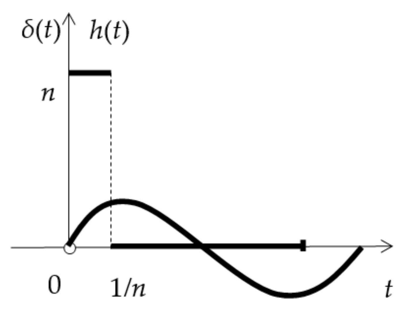
The Dirac function δ(t) is a function that is zero everywhere except the point t = 0. In practice, the Dirac function δn(t) is used:
for which:
0 t < 0
δn(t) = n pre 0 ≤ t ≤ 1/n,
0 t >1/n
δn(t) = n pre 0 ≤ t ≤ 1/n,
0 t >1/n
The Laplace transform of the Dirac function is:
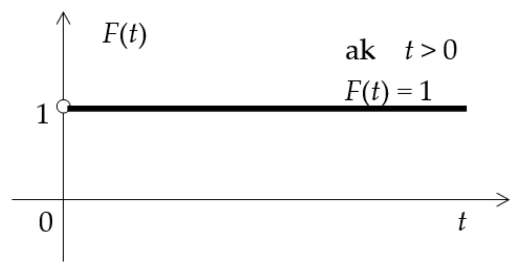
The transition function H(t) is defined as the response to the excitation in the form of a unit jump (Figure 5):
By this the linear system is mathematically described in the time domain.
A mathematical description of a linear system in the frequency domain can also be conducted by means of the frequency response function H(p), which is defined as a Laplace transform of the weight function h(t):
where p is complex variable and L is operator of Laplace transform.
The frequency response of a linear system (FRF H(p) for p = i·ω) is introduced as the ratio of the steady response to the harmonic excitation:
If the input quantity is periodic with a unit amplitude:
it is possible to write for the output quantity:
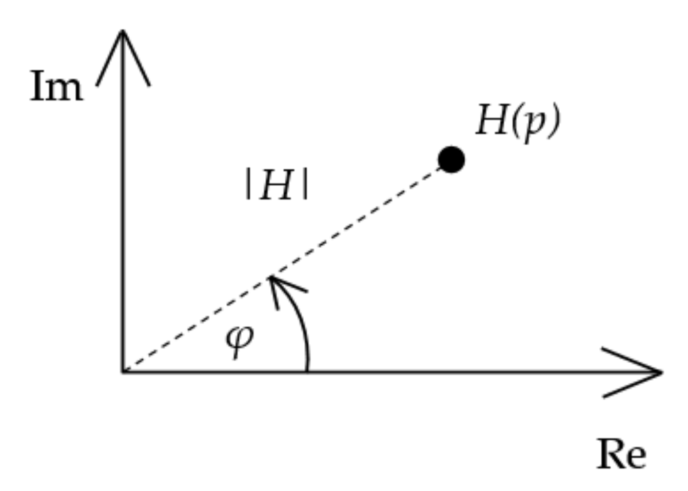
The frequency response H(i·ω) is a complex function, and can be recorded as a vector sum of the real part Re[H(i·ω)] and the imaginary part Im[H(i·ω)] (Figure 6):
or:
where |H(i.ω)| is the absolute value or magnitude of the FRF, and means the amplitude of the response r(t) of the system excited by a simple harmonic function according to (19). In Equation (22), φ means the phase of FRF, that is, the phase of response r(t).
After substituting (22) into (20), we obtain:
These relations are valid:
and:
4.4. FRF of the Beam Bridge Model with Three DOF
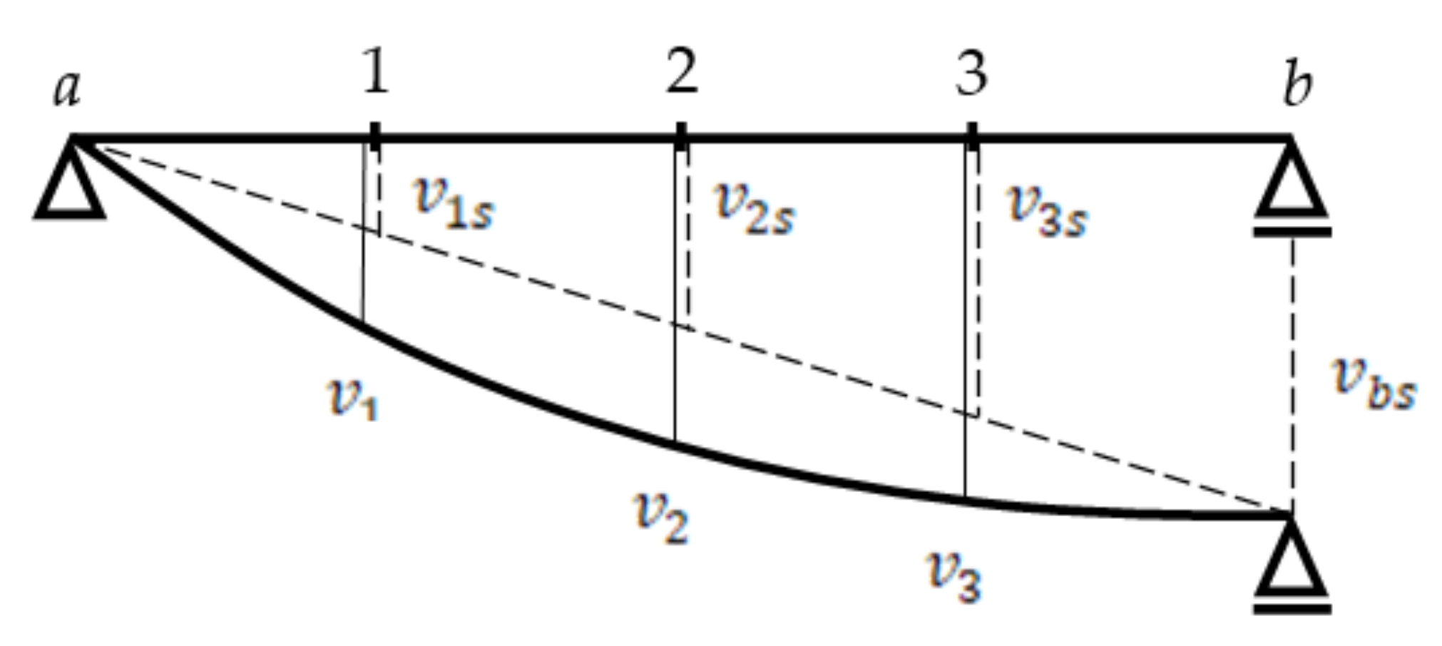
Consider a beam computational model of a bridge with three DOF (Figure 7). Assume that the right beam support (point b) moves in a vertical direction because of harmonic motion:
Point 1 at 1/4 of the span from the support a then performs a vertical harmonic motion:
Point 2 at 2/4 of the span from the support a then performs a vertical harmonic motion:
Point 3 at 3/4 of the span from the support a then performs a vertical harmonic motion:
If vbs = 1, then v1s = vbs/4 = 1/4,
v2s = 2·vbs/4 = 2/4,
v3s = 3·vbs/4 = 3/4.
v3s = 3·vbs/4 = 3/4.
The equations of motion have the form:
After substituting for v1k(t), v2k(t), v3k(t) and adjusting we obtain:
Respectively:
Based on the Fourier transform, the equations of motion will be transformed from the time to the frequency domain, as follows:
Let us define FRF as follows:
Divide each of the equations of motion by a value Vbk(q) and obtain:
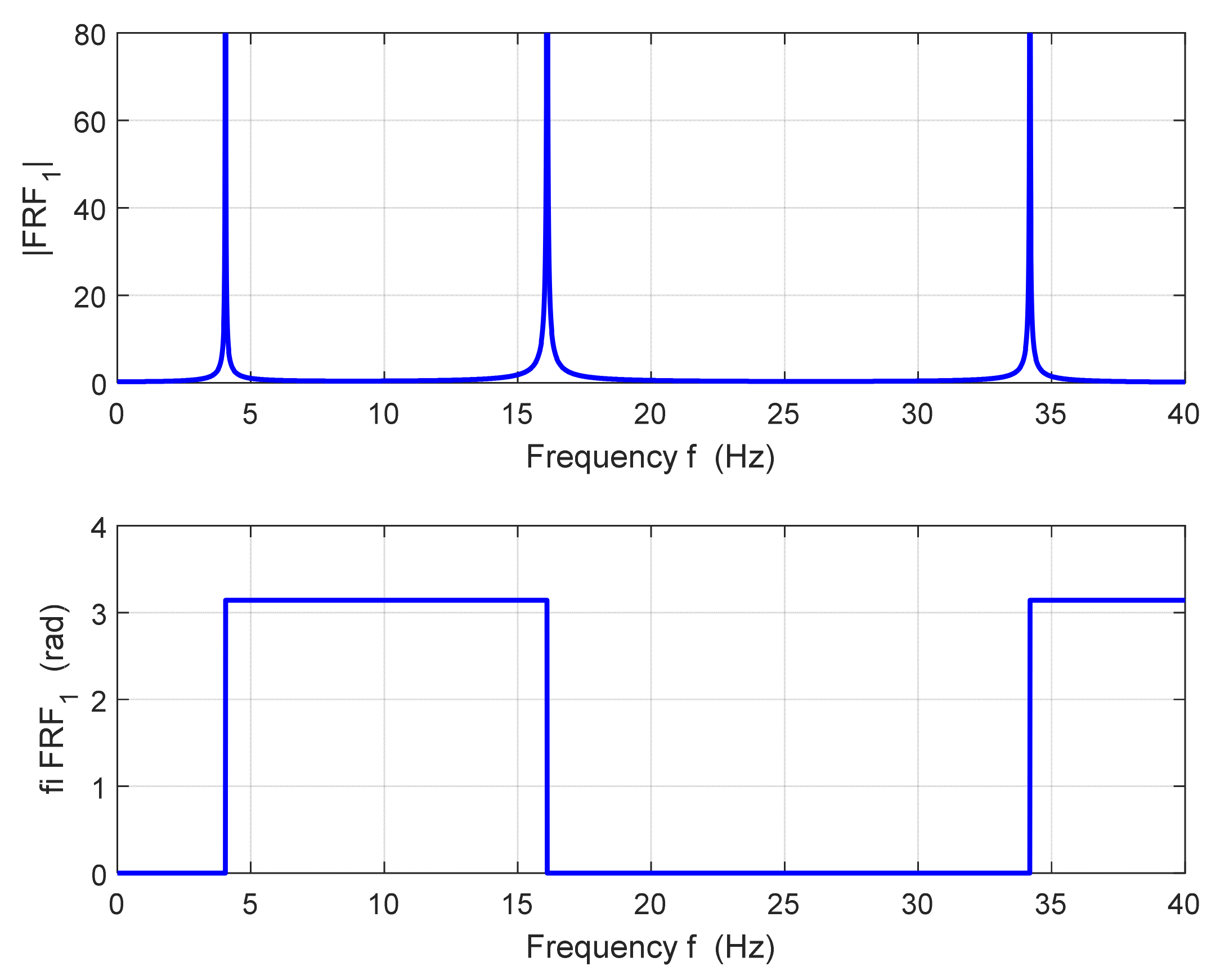
By solving the system of Equation (35) in the frequency band 0 ÷ 40 Hz, the amplitude and phase characteristics are calculated. A frequency step of 0.01 Hz was used for the calculation. The absolute value (magnitude) of the frequency response function at point 1 (|FRF1|≡ ||) and its phase (fi FRF1 ≡ φ1) are plotted in Figure 8. FRF is a complex function. In our particular case, the functions (i = 1, 2, 3) are real functions. That is all right, because an undamped system can only vibrate in phase or in antiphase, φi = 0 or π (i = 1, 2, 3). The vector (i = 1,2,3), therefore, has only a real component, which represents the special case of a complex number.
The spikes of the || function correspond to the frequencies 4.04 Hz, 16.16 Hz, and 36.36 Hz. The function || has points of discontinuity (vertical asymptotes) in these places. Their position corresponds to the values of natural frequencies of the system.
4.5. FRF of the Beam Bridge Model with Continuously Distributed Mass (CDM)
The equation of a bending line, describing the amplitude of the steady-state forced vibration of a single supported beam, has the shape:
In the case of kinematic excitation at the right support point according to Equation (37):
The integration constants have the following form:
Then, it is possible to rewrite Equation (36) into the form:
Equation (39) depends not only on the x-coordinate, but also on the frequency f. Let us introduce FRF as:
After dividing Equation (39) by the value vbs, we can write:
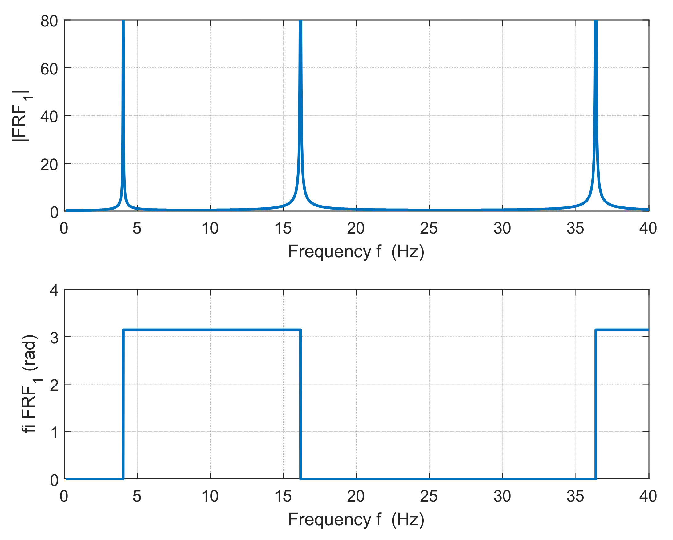
We will enumerate the values points x = l/4, x = l/2, and x = 3l/4, which are for the dimensionless coordinates x/l = 0.25, x/l = 0.5, and x/l = 0.75. The calculations will be performed in the frequency band f = 0 ÷ 40 Hz with a step Δf = 0.01 Hz, f = ω/(2π). The observed amplitude and phase characteristics for point 1 are plotted in Figure 9, where (|FRF1|≡ | (l/4)| fi FRF1 ≡ φ1). The functions have discontinuity points in places of natural frequencies f(1) = 4.0401 Hz, f(2) = 16.1605 Hz, and f(3) = 36.3612. Theoretically, they reach infinitely large values here.
5. Rayleigh’s Energy Method (REM)
The energy method is used to make a qualified estimate of the first natural frequency of the system. It is based on the law on the conservation of mechanical energy [10]:
where is the estimate of the first natural mode of the vibration. Substituting (43) and (44) into (42), we obtain:
In the case of beam structures, it is possible to use the influence line (IL) of deflection for the middle of the beam span or the bending line (BL) from the self-weight as an estimate of the first natural mode of vibration. The energy method gives a higher value of the natural frequency than the exact solution. The first case gives the value of the first natural frequency of 4.06 Hz, and the second case the value of 4.04 Hz.
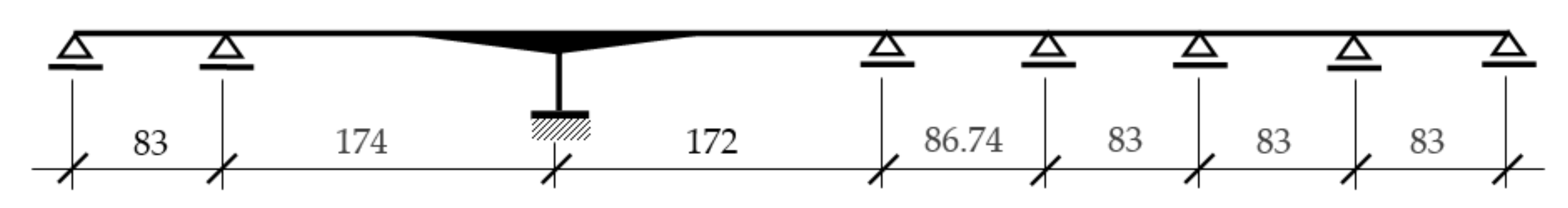
A qualified estimate of the first natural frequency is important if the FEM is not used for the calculation of the eigenvalues. For example, for the calculation of the eigenvalues of the Lafranconi bridge, crossing the Danube in Bratislava, the Kolousek’s slope deflection method was used [11]. At that time, FEM could not be used for dynamic analysis in Slovakia. A simple schema of the bridge is shown in Figure 10. The first natural frequency evaluated by REM was 1.027 Hz. The experiment confirmed the value of 0.875 Hz. Knowledge of the first natural frequency significantly streamlined the calculation process.
6. Experimental Test
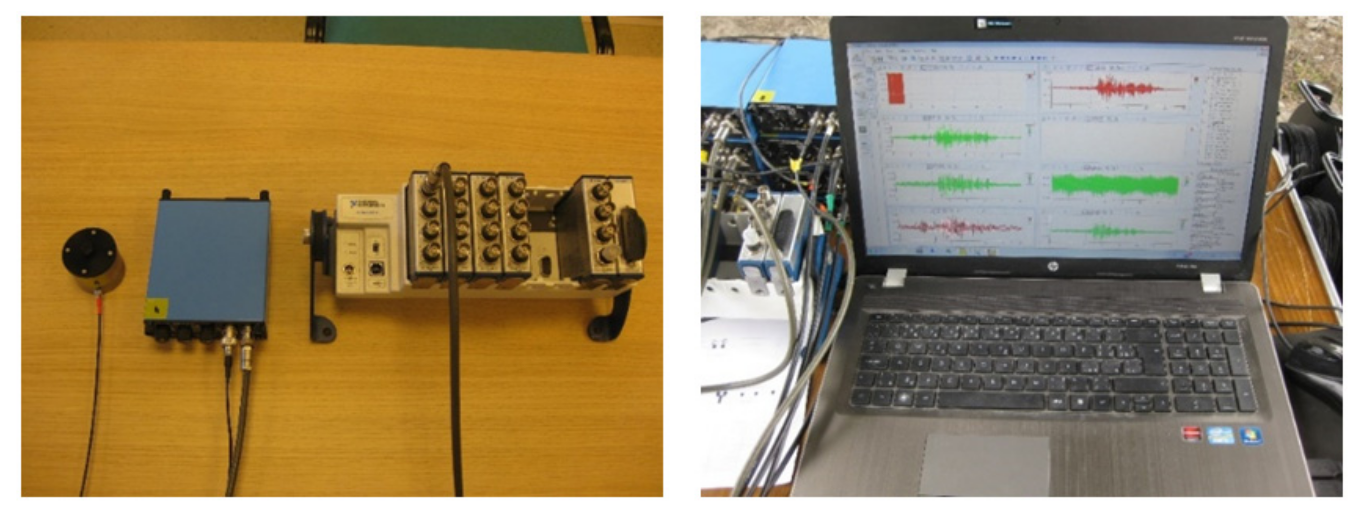
The following experiment was performed to verify the values of some of the calculated natural frequencies. The response of the bridge to the technical seismicity caused by railway traffic under the bridge was monitored. KB12VD 15,040 accelerometers from Metra Mess and Frequenztechnik (MMF) were used to measure the response. This is a classic accelerometer that uses a piezoelectric effect. The sensors operate in the frequency range from 0.15 to 260 Hz. The signal from the sensor is amplified by the charge amplifier M68, also a product of MMF. The amplifier also serves as an integrating member and a low-pass filter. The signal is further digitized in an analog-to-digital converter (A/D converter National Instruments NI 9215) and enters the computer in numerical form, where it is stored and further processed. The complete set of instruments, including the computer, is shown in Figure 11.
Signal digitization was performed with a sampling frequency of fV = 1000 Hz. According to Shannon’s theorem [12], the highest signal frequency before digitization must be less than half the sampling frequency (Nyquist frequency fN = fV/2 = 500 Hz). To achieve the highest signal measurement accuracy in the time domain, the M68 amplifier manufacturer recommends setting the cut-off frequency of the low-pass filter to one-tenth of the sampling frequency. In our case, it is 100 Hz. The signal is digitized only after such filtering.
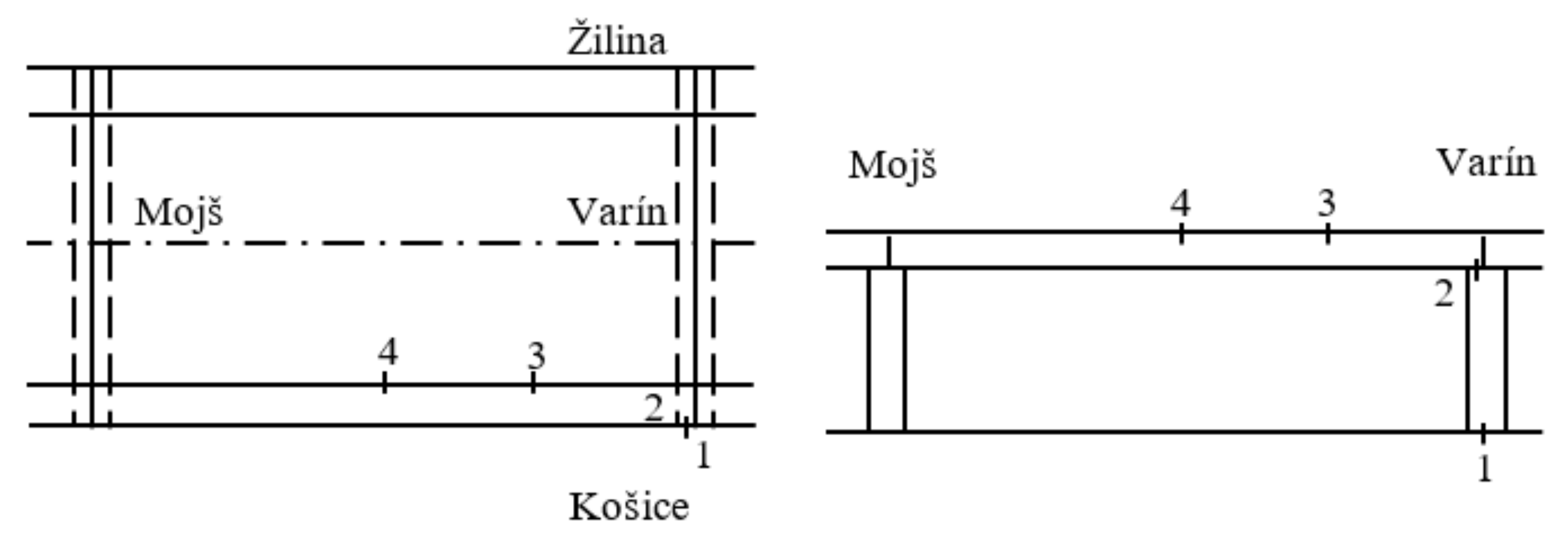
The localization of the sensors on the second bridge field is shown in Figure 12 (top view on the left, side view on the right). Sensor 2 was placed above the support, sensor 3 at 1/4 of the span, and sensor 4 at 1/2 of the span. A total of eight measurements were carried out. The vibrations of the bridge were registered during the passage of eight trains under the first field of the bridge. Spectral analysis (Power Spectral Densities—PSD) was performed from the monitored records using the DISYS system [13]. Discrete Fourier Transform (DFT) was used to calculate the PSD. The length of the records ranged from about 60 to 200 s which, at a sampling frequency of 1000 Hz, represents 60,000–200,000 samples. The algorithm works with the number of 2n samples. The power of n was in an interval from 16 to 18. The detected values of frequencies with a dominant position (interval and average value) are given in Table 3. The experiment was realized in April 2016.
It is interesting to note that in the experiment performed in August 2009, the experimentally verified value of the first natural frequency ranged from 4.042 to 4.048 Hz, which is practically identical to the result of the numerical calculation 4.04 Hz. The difference in the measured frequencies in 2009 and 2016 can have two causes. The first reason may be a change in the temperature at which the experiment was performed. In 2009, the air temperature was 28 °C and in 2016, it was only 8 °C. A change in temperature of 20 °C could affect the value of the first natural frequency by 0.08 Hz. The second reason could be that a completely different measuring string was used in the 2016 experiment. Relative deflections in the middle of the bridge span were measured. The natural frequencies were evaluated from the record of the free vibration of the structure after the vehicle left the bridge. However, a combination of both causes is most likely.
7. Conclusions
For a dynamic analysis of bridge structures, it is often necessary to know the lowest natural frequencies of the bridge vibration. FEM is most often used for their calculation. However, there are other procedures. For example, FRF can be used to determine the natural frequencies of bending vibration, and REM provides a very good estimate of the first natural frequency. The possibility of experimental verification is always welcome. It provides engineers with the assurance that their numerical solutions are correct. In this case, a frequency analysis of the random vibration of the bridge due to seismic excitation induced by railway traffic was used for experimental verification. A comparison of the calculated and experimentally confirmed natural frequencies of the bending oscillation of the bridge is shown in Table 4. The table also shows the percentage differences of the individual frequencies compared to the experiment. A comparison between the calculated and experimentally verified natural frequencies clearly shows that the first natural frequency is calculated most accurately using any method.
Many workplaces are not equipped to perform FEM analysis or experimental modal analysis. Therefore, simpler alternative procedures are welcome for engineers in praxis, especially at the time of growing the need to reconstruct old bridges. This article seeks to provide engineers with the proven simpler calculation alternatives and, at the same time, arouse their interest in a deeper mathematical analysis of the problem.
Author Contributions
Conceptualization, J.M. and V.V.; methodology, J.M.; software, V.V.; validation, J.M. and V.V.; formal analysis, V.V.; investigation, J.M.; resources, V.V.; data curation, J.M.; writing—original draft preparation, J.M. and V.V.; writing—review and editing, V.V.; visualization, V.V.; supervision, J.M.; project administration, J.M.; funding acquisition, J.M. and V.V. All authors have read and agreed to the published version of the manuscript.
Funding
This research was funded by the Grant National Agency of the Slovak Republic VEGA, grant number 1/0006/20.
Data Availability Statement
In this section, please provide details regarding where data supporting reported results can be found, including links to publicly archived datasets analyzed or those generated during the study. Please refer to suggested Data Availability Statements in section “MDPI Research Data Policies” at https://0-www-mdpi-com.brum.beds.ac.uk/ethics, accessed on 14 December 2021. You might choose to exclude this statement if the study did not report any data.
Acknowledgments
This paper was supported by the Grant National Agency VEGA of the Slovak Republic, grant No. 1/0006/20.
Conflicts of Interest
The authors declare no conflict of interest.
References
- Bathe, K.J. Finite Element Procedures, 2nd ed.; Klaus-Jürgen Bathe: Watertown, MA, USA, 2014; Available online: https://www.amazon.com/Finite-Element-Procedures-Klaus-J%C3%BCrgen-Bathe/dp/0979004950 (accessed on 14 December 2021).
- Maia, N.M.M.; Silva, J.M.M. Theoretical and Experimental Modal Analysis; Research Studies Press: New York, NY, USA, 1997. [Google Scholar]
- Ewins, D.J. Modal Testing, Theory, Practice, and Application; Research Studies Press: New York, NY, USA, 2000. [Google Scholar]
- Friswell, M.; Mottershead, J.E. Finite Element Model Updating in Structural Dynamics; Springer Science& Business Media: Berlin/Heidelberg, Germany, 1996. [Google Scholar]
- Hemez, F.M.; Farrar, C.R. A Brief History of 30 Years of Model Updating in Structural Dynamics. In Special Topics in Structural Dynamics; Springer: Berlin/Heidelberg, Germany, 2014; Volume 6, pp. 53–71. [Google Scholar]
- Sehgal, S.; Kumar, H. Structural Dynamic Model Updating Techniques: A State of the Art Review. Arch. Comput. Methods Eng. 2016, 23, 515–533. [Google Scholar] [CrossRef]
- Sestieri, A.; d´Ambrogio, W. Frequency Response Function versus Output-Only Modal Testing Identification. In Proceedings of the 21st International Modal Analysis Conference, Orlando, FL, USA, 3–6 February 2003; pp. 41–46. [Google Scholar]
- Chopra, A.K. Dynamics of Structures. In Theory and Applications to Earthquake Engineering, 4th ed.; Pearson Education, Prentice Hall: Hoboken, NJ, USA, 2012; Available online: https://0-scholar-google-com.brum.beds.ac.uk/scholar_lookup?hl=en&publication_year=2016&pages=374&author=J.+Melcer&title=Dynamics+of+Transport+Structures+%28in+Slovak%29 (accessed on 14 December 2021).
- Němec, I. NE-11, Spatial Structures Composed of Slab-Wall and Beam Elements; Prostorové konstrukce složené z deskostěnových a prutových prvků, Dopravoprojekt: Brno, Czech Republic, 1990. (In Czech) [Google Scholar]
- Melcer, J. Dynamics of Transport Structures; EDIS, University of Žilina: Žilina, Slovakia, 2016. [Google Scholar]
- Bendat, J.S.; Piersol, A.G. Random Data, Analysis and Measurement Procedures; John Wiley & Sons: Hoboken, NJ, USA, 2010. [Google Scholar]
- DISYS Software for Data Acquisition & Analysis; MERLIN, s.r.o.: Prague, Czech Republic, 1993.
- Melcer, J. Dynamic Calculation of the Bridge D 201 HMO Crossing the Danube in Bratislava–Right Bridge; VŠDS: Žilina, Slovakia, 1989. [Google Scholar]
Figure 1.
Cross-section of the bridge. Dimensions in mm.

Figure 2.
Cross-sectional dimensions in mm.

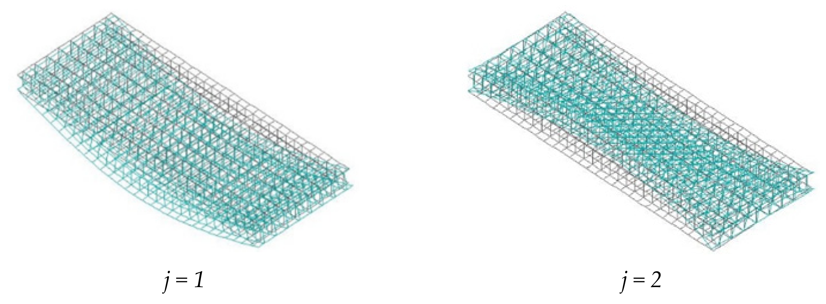
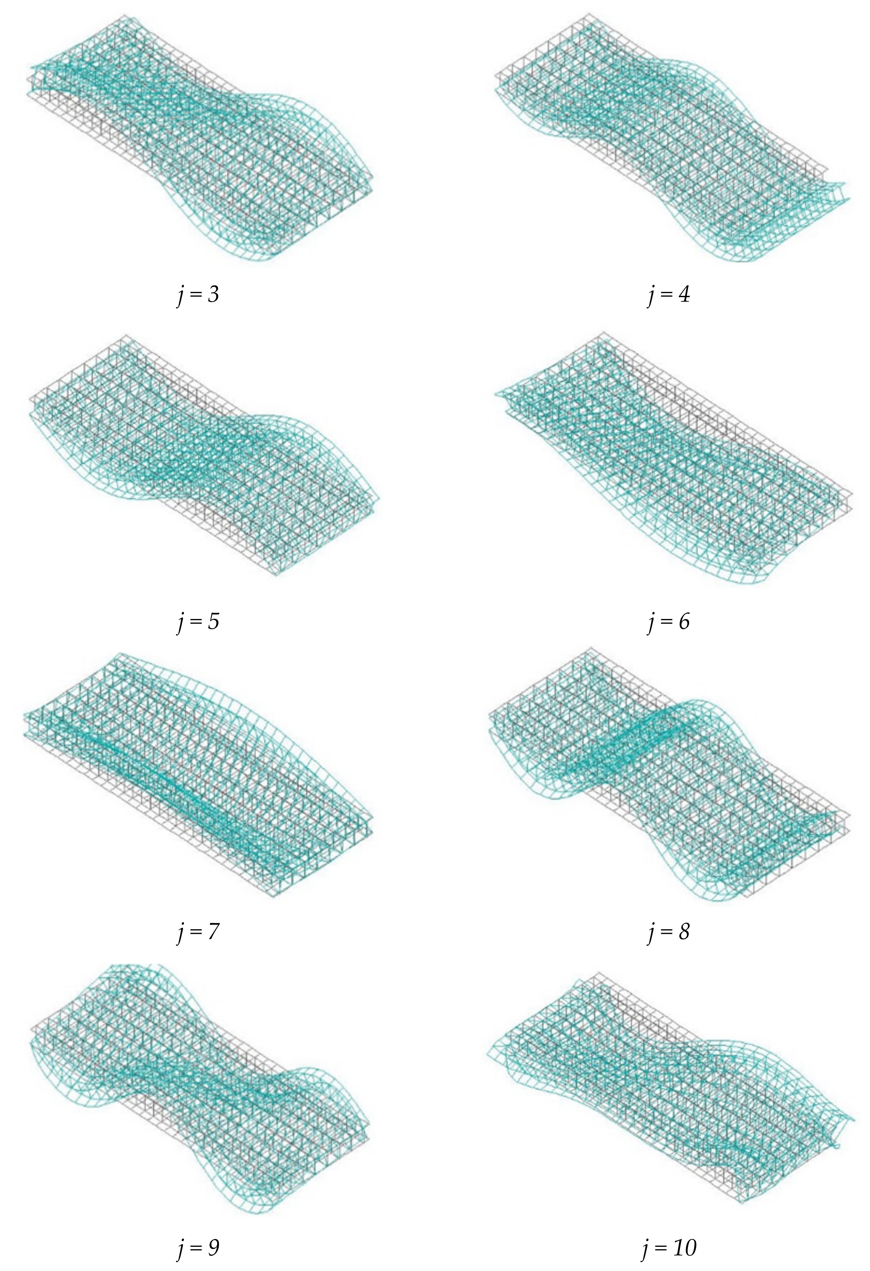
Figure 3.
Natural modes of the bridge.


Figure 4.
Dirac function δn(t) and weight function h(t) for the SDF system.

Figure 5.
Excitation force in the form of a unit jump.

Figure 6.
FRF in complex form.

Figure 7.
Kinematic excitation at point b, the computational model with 3 DOF.

Figure 8.
Amplitude and phase characteristics of FRF at point 1, with 3 DOF.

Figure 9.
Amplitude and phase characteristics of FRF at point 1, CDM.

Figure 10.
A simple schema of the Lafranconi bridge. Dimensions in m.

Figure 11.
Sensor, amplifier, A/D converter, and operative computer.

Figure 12.
Sensor localization.


Table 1.
Cross-sectional dimensions.
| Type - | Dimensions (m) | Number - | Area Mass Density μ (kg/m2) | Mass Moment of Inertia Im per Unit Area (kg) |
|---|---|---|---|---|
| T1 | 1 × 0.72 × 0.135 | 58 | 388.88890 | 0.5733 |
| T2 | 1 × 1.44 × 0.135 | 203 | 388.88890 | 0.5733 |
| T3 | 1 × 1.3566 × 0.22 | 232 | 502.01840 | 2.2232 |
| T4 | 1 × 0.72 × 0.5 | 116 | 1060.59030 | 14.7125 |
| T5 | 1 × 0.72 × 0.2 | 58 | 772.39584 | 6.5090 |
| T6 | 1 × 1.44 × 0.2 | 145 | 772.39584 | 6.5090 |
Table 2.
Natural frequencies calculated by FEM.
| j - | f(j) (Hz) | Node - | j - | f(j) (Hz) | Node - |
|---|---|---|---|---|---|
| 1 | 4.04 | 1st bending | 6 | 26.61 | axial-bending |
| 2 | 10.59 | 1st torsional | 7 | 34.23 | 1st bubble |
| 3 | 14.89 | 2nd bending | 8 | 38.82 | 3rd bending |
| 4 | 19.44 | 2nd torsional | 9 | 39.01 | 4st torsional |
| 5 | 23.29 | 3rd torsional | 10 | 43.79 | 5st torsional |
Table 3.
Natural frequencies obtained from experiment.
| Dominant Frequencies in (Hz) | |||||
|---|---|---|---|---|---|
| Interval | 4.11–4.14 | 9.02–9.27 | 14.12–14.87 | 18.30–23.64 | 36.25–36.60 |
| Average value | 4.12 | 9.15 | 14.29 | 19.38 | 36.41 |
Table 4.
Selected natural frequencies of the bridge.
| Natural Frequencies f(j) in Hz | ||||||
|---|---|---|---|---|---|---|
| Node j | FEM | FRF—3 DOF | FRF—CDM | REM IL | REM BL | Experiment |
| 1st bending | 4.04 (−1.94%) | 4.04 (−1.94%) | 4.04 (−1.94%) | 4.06 (−1.45%) | 4.04 (−1.94%) | 4.12 |
| 2nd bending | 14.89 (+4.20%) | 16.04 (+12.25%) | 16.16 (+13.09%) | - | - | 14.29 |
| 3rd bending | 38.82 (+6.62%) | 34.06 (−6.45%) | 36.36 (−0.14%) | - | - | 36.41 |
Publisher’s Note: MDPI stays neutral with regard to jurisdictional claims in published maps and institutional affiliations. |
© 2022 by the authors. Licensee MDPI, Basel, Switzerland. This article is an open access article distributed under the terms and conditions of the Creative Commons Attribution (CC BY) license (https://creativecommons.org/licenses/by/4.0/).
Share and Cite
MDPI and ACS Style
Valašková, V.; Melcer, J. Bridge Natural Frequencies, Numerical Solution versus Experiment. Appl. Sci. 2022, 12, 1765. https://0-doi-org.brum.beds.ac.uk/10.3390/app12031765
AMA Style
Valašková V, Melcer J. Bridge Natural Frequencies, Numerical Solution versus Experiment. Applied Sciences. 2022; 12(3):1765. https://0-doi-org.brum.beds.ac.uk/10.3390/app12031765
Chicago/Turabian StyleValašková, Veronika, and Jozef Melcer. 2022. "Bridge Natural Frequencies, Numerical Solution versus Experiment" Applied Sciences 12, no. 3: 1765. https://0-doi-org.brum.beds.ac.uk/10.3390/app12031765
Note that from the first issue of 2016, this journal uses article numbers instead of page numbers. See further details here.