Stock Portfolio Management in the Presence of Downtrends Using Computational Intelligence

Abstract

Stock portfolio management consists of defining how some investment resources should be allocated to a set of stocks. It is an important component in the functioning of modern societies throughout the world. However, it faces important theoretical and practical challenges. The contribution of this work is two-fold: first, to describe an approach that comprehensively addresses the main activities carried out by practitioners during portfolio management (price forecasting, stock selection and portfolio optimization) and, second, to consider uptrends and downtrends in prices. Both aspects are relevant for practitioners but, to the best of our knowledge, the literature does not have an approach addressing them together. We propose to do it by exploiting various computational intelligence techniques. The assessment of the proposal shows that further improvements to the procedure are obtained when considering downtrends and that the procedure allows obtaining portfolios with better returns than those produced by the considered benchmarks. These results indicate that practitioners should consider the proposed procedure as a complement to their current methodologies in managing stock portfolios.

1. Introduction

Both individual and organizational investors commonly seek to take profits from stock markets. Among the different ways to exploit these markets, the literature has focused on the idea of buying cheap and selling expensive. The authors of [1] point out that there is an assumption in classical portfolio theory to manage the selected assets with the simplest trading strategy, which is a buy-and-hold approach. However, it is also common for practitioners to also seek profits when prices go down. There are several mechanisms that allow an investor to take profits in this situation (e.g., [2,3,4]).

Investing in stocks when their prices are expected to rise is known as opening a long position. In this scenario, the investor adopts the idea that stocks should be bought when they are the cheapest and sold when they are as expensive as possible; the difference between selling and buying prices constitutes the investor’s basic earning. On the other hand, opening a short position means that the investor expects the stock prices to go down. According to [5], short selling allows the investor to profit from their belief that the price of a security will decline. Moreover, short selling is used by top-down and quantitative managers as a part of a neutral strategy (cf. [5]). In this case, the investor can, for example, borrow shares of the stock, sell them in this very moment and commit to return them at a moment in the future; so, to return them, the investor will have to buy them at whatever the price of the stock is at that moment in the future. Therefore, the earning of the investment here is also calculated as the difference between the selling and buying prices—just that the sell is produced first.

The highly complex decision-making process of allocating resources considering both uptrends and downtrends of prices requires sophisticated models and tools to achieve competitive results. Thus, this work proposes a comprehensive procedure based on computational intelligence that aids defining how investors should allocate their resources in the presence of both scenarios.

First, an artificial neural network (ANN) (cf. [6]) is used to estimate future prices. There are evident tendencies in the literature showing that ANNs have high accuracy, fast prediction speed and clear superiority in predictions related to financial markets (e.g., [7,8,9]). To perform these estimations, the ANN takes historical performances of the stocks considering the most common factors of the literature, such as stock prices and financial ratios (cf. [10]). Some additional financial indicators are used here to determine if the forecasted tendency (that the price will go up or down) is supported. These indicators are taken from the so-called fundamental analysis, a type of indicators often considered by practitioners (cf. [11]). Evolutionary algorithms (EAs) are then used to ponder these indicators altogether with the price estimation and determine which stocks should be considered by the investor for investment, either with a downtrend or an uptrend. Finally, EAs are also used to determine how much of the resources should be allocated to each of the selected stocks on the basis of statistical analysis to historical data. Here, only historical prices of the selected stocks are taken into consideration according to the approach described in [12].

The literature review presented in Section 3 shows that, although there are studies that consider both uptrends and downtrends in stock prices, as far as we know, there are no published works that comprehensively address the problem the way that is proposed here. That is, not only taking advantage of a future increase in prices by opening long positions but also taking advantage of future decrease in prices by opening short positions, while also forecasting stock prices, selecting the most plausible stocks and optimizing the stock portfolio. Our hypothesis is that a procedure that effectively implements all this provides better overall earnings for the investor. The hypothesis is based on the activities and interests of practitioners. We test this hypothesis by using extensive experiments with actual historical data.

The rest of the paper is structured as follows. Section 2 describes the fundamental theories that support this research. Section 3 presents the related literature. Section 4 describes the details of the techniques that compose the proposed procedure. In Section 5, we explained the experiments to test this work’s hypothesis. Finally, Section 6 concludes this paper.

2. Background

This section provides a brief overview of the concepts and methods used in the proposed approach. These concepts and methods are (i) fundamental analysis, (ii) artificial neural networks and (iii) evolutionary multi-objective optimization. Furthermore, we provide a short description of multiobjective optimization problems in order to present a complete theoretical basis of the proposed approach.

2.1. Fundamental Analysis

One of the most used sources of information in the management of stock portfolios comes from the so-called fundamental analysis. The fundamental indicators provided by this analysis allow the practitioner to evaluate stocks from multiple perspectives. Such indicators are constructed from the financial statements that the companies (underlying the stocks) present publicly on a regular basis.

Fundamental indicators provide information that is often exploited in the literature to forecast future stock performance and to select the most competitive stocks. These indicators can be used both qualitatively and quantitatively. Regarding the latter, the financial information published by companies is synthesized in the form of ratios that shed light on the current state of the company, providing remarkable information on what can be expected from the financial health of the company and the possible future price of its stock. When this analysis is used in the literature, the fundamental indicators are usually aggregated in an overall assessment value that requires subjective preferences from the practitioner (cf. e.g., [13]); however, the aggregation procedure is not straightforward and represents an important challenge.

On the other hand, different fundamental indicators could be more convenient for companies with different types of activities ([14]). Some fundamental indicators that can be used for trans-business companies are described in Section 4.1 (cf. [10,11,13,14]).

2.2. Artificial Neural Networks

Artificial neural networks are nowadays very popular among techniques from computational intelligence that have been used for many applications, such as classification, clustering, pattern recognition and prediction in diverse scientific and technological disciplines ([15,16]). Similarly to other computational intelligence techniques, applications of ANN are very diversified due to its capability to model systems and phenomena from the fields of sciences, engineering and social sciences.

Analogously to a nervous system, an ANN is built from neurons, which are the basic elements for processing signals. Neurons are interconnected to form a network, with additional connections (synaptic relations) for input and output signals. Weights are assigned to each of these and other connection. The computing of suitable values for these weights is performed by training algorithms. An ANN needs to be trained before it can be used by using data from the system or phenomenon to model. Neurons are configured to form layers, in which neurons have parallel connections for inputs and outputs. ANN complexity varies from a network with a single layer of a single neuron to networks with several layers, each having several neurons. Networks with only forward connections are known as feedforward networks. Networks with forward and backward connections are known as feedbackward networks ([15]). The term deep learning refers to ANN with complex multilayers ([17]). Roughly speaking, deep learning has more complex connections between layers and also more neurons than previous types of networks. Some neural networks that form deep learning networks are convolutional networks, recursive networks and recurrent networks.

2.3. Multi-Objective Optimization Problem

Without loss of generality, a multi-objective optimization problem (MOP) can be defined in terms of maximization (although minimization is also common) as follows:

$$\mathrm{maximize}F\left(x\right)={[f_1\left(x\right),f_2\left(x\right),\dots ,f_k\left(x\right)]}^{\top }$$

$$\mathrm{subject}\mathrm{to}x\in \Omega$$

where $\Omega$ is the set of decision variable vectors $x=[x_1,x_2,\dots ,x_m){]}^{\top }$ that fulfill the set of constraints of the problem, and then $F:\Omega \to {\mathbb{R}}^k$, where ${\mathbb{R}}^k$ is the so-called objective space.

It is evident that the notation used here states that all functions $f_i$ (objectives) should be maximized; however, it is also possible that one requires some functions $f_i$ to be minimized instead. To keep standard notation, we assume that the latter can be simply achieved by multiplying the minimizing function by $-1$.

In the context of stock portfolio management, the functions $f_i$ are usually in conflict with each other. This means that improving $f_j$ deteriorates $f_k$ for some $j\ne k$. Therefore, there is no solution $x\in \Omega$ that maximizes all the k objectives simultaneously. Nevertheless, it is still possible to define some solutions x that poses the best characteristics in terms of their impact on the objectives; this is commonly carried out through Pareto optimality (cf. [18]).

Let $u,\mathrm{vs}.\in {\mathbb{R}}^k$ denote impacts of solutions x and y, respectively. u dominates v if and only if $u_i\ge v_i$ for all $i=1,\dots ,k$, and $u_j>v_j$ for at least one $j=1,\dots ,k$. Then, a solution $x^{*}\in \Omega$ is Pareto optimal if there is no solution $y\in \Omega$ such that $F\left(y\right)$ dominates $F\left(x^{*}\right)$. Note that there can be more than one Pareto optimal solution. The set of all the Pareto optimal solutions is called the Pareto set (PS), and the set of all their corresponding objective vectors is the Pareto front (PF).

2.4. Evolutionary Multi-Objective Optimization

Multi-objective evolutionary algorithms (MOEAs) are high-level procedures designed to discover good enough solutions to MOPs (solutions that are close to the global optimum). They are especially useful with incomplete or imperfect information or a limited computing capacity ([19]).

MOEAs address MOPs using principles from biological evolution. They use a population of individuals, each representing a solution to the MOP. The individuals in the population reproduce among them, using so-called evolutionary operators (selection, crossover, mutation), to produce a new generation of individuals. Often, this new generation of individuals is composed of both parents and children that posses the best fitness; this fitness represents the impact on the objectives of the MOP. Since each individual encodes a solution to the MOP, MOEAs can approximate a set of trade-off alternatives simultaneously.

The performance of MOEAs has been assessed in different fields (e.g., [20,21]). They have been widely accepted as convenient tools for addressing the problem of stock portfolio management ([10,11,12]). The main goal of MOEAs is to find a set of solutions that approximate the true Pareto front in terms of convergence and diversity. Convergence refers to determining the solutions that belong to the PF, while diversity refers to determining the solutions that best represent all the PF. Thus, the intervention of the decision maker is not traditionally used in the process. Thus, rather little interest has been paid in the literature to choosing one of the efficient solutions as the final one in contrast to the interest paid in approximating the whole Pareto front.

Usually, two types of MOEAs are highlighted in the literature: differential evolution and genetic algorithms. Differential evolution (DE) has been found to be very simple and effective ([22]), particularly when addressing non-linear single-objective optimization problems ([23,24]). On the other hand, in a genetic algorithm (GA), solutions to a problem are sought in the form of strings of characters (the best representations are usually those that reflect something about the problem that is being addressed), virtually always applying recombination operators such as crossing, selection and mutation operators. GAs compose one of the most popular meta-heuristics applied to the Portfolio Optimization Problem ([12]).

As a very effective and efficient way to address MOPs, the authors of ([25]) exploited the idea of creating subproblems underlying the original optimization problem. This way, addressing these subproblems the algorithm proposed in ([25]) indirectly addresses the original problem. In that work, the so-called Multiobjective Evolutionary Algorithm Based on Decomposition (MOEA/D) was presented. The goal of MOEA/D is to create subproblems such that, for each subproblem, a simpler optimization problem can be more effectively and efficiently addressed; each subproblem consists on the aggregation of all the objectives through a scalar function. MOEA/D was extended to the context of interval numbers in [12].

3. Literature Review

There are many contributions to portfolio management literature in recent years. In this section, we give an overview of some recent and relevant works on the following subjects: price forecasting, stock selection and portfolio optimization, as well as works on portfolio management by algorithms that exploits both uptrends and downtrends in stock prices.

Due to the non-linearity of stock data, a model developed using traditional approaches with single intelligent techniques may not use the resources in an effective way. Therefore, there is a need for developing a hybridization of intelligent techniques for an effective predictive model [26].

3.1. Portfolio Management: Price Forecasting, Stock Selection and Portfolio Optimization

In recent years, there have been plenty of contributions on price forecasting based on either statistical or computational intelligence methods (see [10,27]). The stock market is characterized by extreme fluctuations, non-linearity, and shifts in internal and external environmental variables. Artificial intelligence techniques can detect such non-linearity, resulting in much-improved forecast results [28].

Among the computational intelligence methods used for price forecasting are deep learning (e.g., [29,30,31,32]) and machine learning (e.g., [33,34,35]). In [10], a hybrid stock selection model with a stock prediction stage based on an artificial neural network (ANN) trained with the extreme learning machine (ELM) training algorithm ([6,36]) was proposed. The ELM algorithm has been tested for financial market prediction in other works (see [7,8,9]).

There are important works on methods for stock selection, which have several different fundamental theories, from operations research methods (e.g., [37,38]) to approaches originating in modern portfolio theory (Mean-variance model) (e.g., [38,39]) and soft computing methods (e.g., [40,41]), including hybrid approaches (e.g., [10,42,43]).

The fundamental theory for portfolio optimization is Markowitz’s mean-variance model ([44]). Its formulation marked the beginning of Modern portfolio theory ([45]). However, Markowitz’s original model is considered too basic since it neglects real-world issues related to investors, trading limitations, portfolio size and others ([43]). For evaluating a portfolio’s performance, the model is based on measuring the expected return and the risk; the latter is represented by the variance in the portfolio’s historical returns. Since the variance takes into account both negative and positive deviations, other risk measures have been proposed, such as the Conditional Value at Risk (CVaR) ([46,47]). As a result, numerous works have improved the model, creating more risk measures and proposing restrictions that bring them closer to practical aspects of stock market trading ([27]). Consequently, many optimization methods based on exact algorithms (e.g., [48,49,50,51,52,53,54,55]) and heuristic and hybrid optimization (e.g., [29,56,57,58,59,60,61,62,63,64,65]) have been proposed to solve the emerging portfolio optimization models ([27,40,45]).

According to [12], the investor or decision maker in the portfolio selection problem manages a multiple criteria problem in which, along with the objective of return maximization, he/she faces the uncertainty of risk. Different attitudes assumed by decision makers may lead them to select different alternatives. A way of modeling both risk and subjectivity of the decision maker in terms of significant confidence intervals was first proposed in [12]. The probabilistic confidence intervals of the portfolio returns characterize the portfolios during the optimization. The optimization is performed by means of a widely accepted decomposition-based evolutionary algorithm, the MOEA/D ([25,66]). This approach is inspired on the independent works of ([67,68]) on interval analysis theory.

3.2. Exploiting Uptrends and Downtrends in Strategies for Stock Investment

Regarding alternative strategies to the known buy-and-hold approach for stock investment, in ([69]), the authors propose two new trading strategies to outperform the buy-and-hold approach, which is based on the efficient market hypothesis. The proposed strategies are based on a generalized time-dependent strategy proposed in ([70]) but propose different timing for changing the buying/selling position. According to ([71]), the decision to adopt a long or short position in an asset requires a view of its immediate future price movements. A typical short seller would have to assess the potential future behavior of the asset price by means of evaluating several factors, such as past returns and market effects as well as and technical indicators, such as market ratios ([71]). There are a few works published in the literature to address the problem of trading strategies for the short position. An interesting work that considers not only the short position but both the short and long position is ([72]), in which a simultaneous long-short trading strategy (SLS) is proposed. Such a strategy is based partially on the property that a positive gain with zero initial investment is expected, which holds for all discrete and continuous price processes with independent multiplicative growth and a constant trend. Other works based on SLS are ([73,74,75]). However, these works show the results of the algorithm on a previously defined stock portfolio, unlike the proposed approach that comprehensively performs price forecasting, stock selection and portfolio optimization in the presence of both uptrends and downtrends.

4. Methods and Materials

The procedure followed here consists of applying several techniques from the so-called computational intelligence to address the complexity of stock investments in the presence of both increasing and decreasing prices. Future stock prices are forecasted using an ANN, as well as the tendency that such prices will show. These estimations are then combined with certain indicators from the fundamental analysis to define the stocks that will likely receive resources (the selected stocks). Finally, another evolutionary algorithm is used to optimize portfolios, i.e., to define the proportions of resources to be allocated to each stock.

4.1. An Artificial Neural Network to Estimate Future Prices

In this work, the immediate next period price of the considered stocks are estimated by means of an ANN. Following the recommendations of ([6,10,36]), we use a single-layer feedforward network (whose setting is created once per each stock) and train the ANN by means of the so-called extreme learning machine algorithm because of its superior capacities in similar problems to the one addressed here (cf. [7,8,9]).

The ANN works independently per stock to estimate its price in the subsequent immediate period. The return of each stock is used as the target variable, while thirteen variables are used as input to train the ANN. Let $r_t$ denote the stock return for a given period t. $r_t$ is calculated from the stock price for that period ($p_t$) and the immediate previous one ($p_{t-1}$), as defined by Equation (1).

$$r_t=\frac{p_t-p_{t-1}}{p_{t-1}}$$

(1)

The high complexity involved in forecasting future stock prices requires one to consider a variety of transaction data as explanatory variables. Therefore, we followed the recommendations provided in ([10,76,77]) to determine sixteen transaction data as explanatory variables to the forecasting model used here. The sixteen input variables are described as follows:

• Close price. Last transacted price of the stock before the market officially closes.
• Open Price. First price of the stock at which it was traded at the open of the period’s trading.
• High. Highest price of the stock in the period’s trading.
• Low. Lowest price of the stock in the period’s trading.
• Average Price. Average price of the stock in the period’s trading.
• Market Capitalization. Price per share multiplied by the number of outstanding shares of a publicly held company.
• Return Rate. Profit on an investment over a period, expressed as a proportion of the original investment.
• Volume. Number of shares traded (or their equivalent in money) of a stock in a given period.
• Total asset turnover. Net sales over the average value of total assets on the company’s balance sheet between the beginning and the end of the period.
• Fixed asset turnover. Net sales over the average value of fixed assets.
• Volatility. Standard deviation of prices.
• General Capital. Number of preferred and common shares that a company is authorized to issue.
• Price to Earnings. Market value per share over earnings per share.
• Price to Book. Market price per share over book value per share.
• Price to Sales. Market price per share over revenue per share.
• Price to Cash Flow. Market price per share over operating cash flow per share.

The training process consists of taking sixty historical values for these sixteen variables randomly out of a set of ninety historical periods and leaving the rest of values to test the ANN. After the ANN is trained, two errors are computed: training error and testing error. The lower the testing error, the better the predictive capacity the ANN has. Nevertheless, since the extreme learning machine algorithm uses a random procedure to compute the weights and bias of the network, we do not always obtain the same results. Therefore, we run the algorithm $n_a$ times and chose the one with better results. It is important to highlight that each input variable is normalized taking into account the sixty periods of the training data (the target variable is not normalized).

As mentioned before, our approach seeks to take advantage of market downtrends. To achieve this, we use the ANN’s forecast. A long or a short position will be chosen according to the forecasted value of the return; that is, if the forecasted value for a stock return is positive, a long position is chosen, otherwise a short position is chosen.

4.2. Evolutionary Algorithms to Select Stocks

It is common that practitioners use indicators from the so-called fundamental analysis to assess the financial health of stocks. Besides these indicators, here, we use the stock prices and tendencies forecasted by the ANN to define which stocks should be further considered for investment. To ponder all these values, we establish an optimization problem following the recommendations in ([78]) and use an evolutionary algorithm to address it as recommended in ([10]).

Let $S=\{s_1,s_2,\dots ,card\left(S\right)\}$ be the set of considered stocks, $v_j\left(s_i\right)$ be the evaluation of stock $s_i$ on the jth indicator, $j=1,\dots ,N$ (for the sake of simplicity, assume that $v_1$ is the forecasted return as calculated by Equation (1)), and $w_i$ be the relative importance of each indicator and forecasted return (the latter is denoted by $w_1$). The score of stock $s_i$ can be calculated as follows (cf. [10,79]):

$$score\left(s_i\right)=\sum _{J=1}^N{w}_j{v}_j\left(s_i\right)$$

(2)

Since increasing $v_j\left(s_i\right)$ for $j=1,\dots ,N$ indicates the convenience of the stock, determining the most appropriate values for $w_j$ becomes crucial to determining the most plausible stocks as those that maximize Equation (2).

If we want to take advantage of market downtrends, sometimes we will be interested in obtaining the more negative returns to invest in a short position. To implement this idea, the value of each factor $v_j$ is taken as positive or negative according to the prediction given by the ANN model on the previous stage. Namely, if the ANN model predicts a positive stock return, a long position will be chosen for this stock and the factor values are taken as they are. However, if the ANN model predicts a negative stock return, a short position is chosen for this stock and the return and each factor value are multiplied by $-1$, so Equation (2) is still valid.

To determine the most convenient values for $w_j$ ($j=1,\dots ,N)$, we use the function recommended in ([78]). Let us define this function.

For a given historical period t, a set of predefined weights will allow one to determine the score of each stock; thus, the top, say, 5% of the stocks can be selected. These top stocks constitute the set of “selected” stocks, and the rest constitute the set of “non-selected” stocks for period t. Let $R_{selected}^t$ and $R_{non-selected}^t$ be the average returns of the stocks in these sets (as calculated by Equation (1)), respectively. The convenience of the predefined weights is then calculated as the arithmetic difference between the average returns of the selected and non-selected stocks that they produce, that is:

$$Maximize\xi \left(W\right)=\frac{1}{T}\sum _{t=1}^T(R_{selected}^t-R_{non-selected}^t)$$

(3)

where T is the number of historical returns used to assess the weights in W, $W={[w_1,w_2,\dots ,w_N]}^{\top }$ and $\xi \left(W\right)$ is the convenience of the weights in W.

As was stated in Section 2.4, the differential evolution (DE) algorithm has been found to be highly effective in non-linear mono-objective optimization problems, especially in problems related to financial problems ([11,23,24]); therefore, this type of algorithm represents serious advantages over other optimization algorithms, particularly over other meta-heuristics. We use here a basic version of the DE algorithm as presented by Algoritm 1 in ([80]). Let us describe this algorithm.

To determine the best values for $w_j$ ($i=1,\dots ,N$), the decision variables considered by the DE will be the values $w_j$ such that each individual in the DE will contain the values for $w_j$ fulfilling the constraints of the problem: $w_j\ge 0$ and ${\sum }_{j=1}^N{w}_j=1$.

Lines 1–8 of Algorithm 1 randomly initialize the population of the DE; that is, the lines initialize feasible individuals by placing them in a random position within the search space. To ensure feasibility, the values for $w_j$ in each individual are normalized in Lines 5 and 6.

The parameters used by the DE algorithm consist of a crossover probability, $CR\in [0,1]$, a differential weight, $F\in [0,2]$, and a number of individuals in the population, $populatio{n}_{size}\ge 4$. Each individual in the population is represented by a real-valued vector $z={[z_1,z_2,\dots ,z_N]}^{\top }$, where $z_j$ is the value assigned to the jth decision variable and N is the number of decision variables (in Problem (2), the decision variables are the N weights). The termination criterion used here for the search procedure consists of a predefined number of iterations (generations). The evolutionary process is performed in Lines 9–22. Here, for each generation of the DE, the solutions in the population are evolved such that the new population is composed of the best solutions found so far. Finally, the best solution found overall is selected in Line 23.

Algorithm 1 Differential evolution used to address Problem (3).

Require:  $N_{iterations}$, $CR$, F, $populatio{n}_{size}$ Ensure:  The values $w_1,w_2,\dots ,w_N$ found that best solves Problem (3) 1: $P\leftarrow \varnothing$ 2: $i\leftarrow 1$ 3: while ($i\le populatio{n}_{size}$) do 4:    Randomly, define $z_k\in [0,1]$ for $z={[z_1,z_2,\dots ,z_N]}^{\top }$ 5:    $sum\leftarrow {\sum }_{k=1}^N{z}_k$ 6:    $z_k\leftarrow z_k/sum$ ($k=1,2,\dots ,N$) 7:    $P\leftarrow P\cup \left\{z\right\}$ 8: end while 9: $j\leftarrow 1$ 10: while ($j\le N_{iterations}$) do 11:    for all ($z\in P$) do 12:       Randomly, define $a,b,c\in P$, such that z, a, b, c are all different 13:       Randomly, define $r\in \{1,\dots ,N\}$ 14:       for all ($i\in \{1,\dots ,N\}$) do 15:          Randomly, define $u\in [0,1]$ 16:          If $u<CR$ or $i=r$, set $y_i=a_i+F·(b_i-c_i)$, otherwise set $y_i=z_i$ 17:       end for 18:       $sum\leftarrow {\sum }_{k=1}^N{y}_k$ 19:       $y_k\leftarrow y_k/sum$ ($k=1,2,\dots ,N$) 20:       If $\xi \left(z\right)\le \xi \left(y\right)$, then replace z for y in P (see Equation (3)) 21:    end for 22: end while 23: Select the individual $z\in P$ with the highest value $\xi \left(z\right)$; this individual represents the best set of weights $w_1,w_2,\dots ,w_N$ for Equation (2).

Different fundamental indicators could be more convenient for companies with different types of activities (see, e.g., [14]). We use here some fundamental indicators that can be used for trans-business companies following the works in ([10,11,13,14]). In this work, we use $N=13$ factors to define the score of each stock as described below.

• Forecasted return: Output of the ANN.
• Return on equity: Net income over average shareholder’s equity.
• Return on asset: Net income over total assets.
• Operating income margin: Operating earnings over revenue.
• Net income margin: Total liabilities over total shareholder’s equity.
• Levered free cash flow: Amount of money the company left over after paying its financial debts.
• Current ratio: Current assets over current liabilities.
• Quick ratio: (Cash and equivalents + marketable securities + accounts receivable) over current liabilities.
• Inventory turnover ratio: Net sales over ending inventory.
• Receivable turnover ratio: Net credit sales over average accounts receivable.
• Operating income growth rate: (Operating income in the current quarter − operating income at the previous quarter) over operating income in the previous quarter.
• Net income growth rate: (Net income after tax in the current quarter − net income after tax at the previous quarter) over net income after tax in the previous quarter.

4.3. Optimizing Stock Portfolios

The final activity to perform stock investments consists of determining how the resources should be allocated. A given distribution of resources among the selected stocks is known as the stock portfolio. Defining the most convenient distribution of resources is known as portfolio optimization. In this final activity, the decision alternatives are no longer individual stocks but complete portfolios. Thus, it is necessary to determine multiple criteria to comprehensively assess portfolios.

Formally, a stock portfolio is a vector $x={[x_1,x_2,\dots ,x_m]}^{\top }$ such that $x_i$ is the proportion of the total investment that is allocated to the ith stock. Let $r_i$ be the return of the ith stock calculated according to Equation (1); the return of a given portfolio x is defined as follows:

$$R\left(x\right)=\sum _{i=1}^m{x}_i{r}_i$$

(4)

Of course, if we knew the $t+1$ return of the stocks, we could allocate resources that maximize $R\left(x\right)$ without uncertainty; however, since this is impossible, the multiple criteria used to assess portfolios are estimations of $R\left(x\right)$. These estimations usually come from probability theory.

According to ([12]), the most convenient portfolio x can be determined by optimizing a set of confidence intervals that describe the probabilistic distribution of the portfolio’s return:

$$\underset{x\in \Omega }{Maximize}\{\theta \left(x\right)=({\theta }_{{\beta }_1}\left(x\right),{\theta }_{{\beta }_2}\left(x\right),\dots ,{\theta }_{{\beta }_k}\left(x\right))\}$$

(5)

where ${\theta }_{{\beta }_i}\left(x\right)=\{[c_i,d_i]:P(c_i\le E\left(R\left(x\right)\right)\le d_i)={\beta }_i\}$, $E\left(R\right(x\left)\right)$ is the expected return of portfolio x, $P\left(\omega \right)$ is the probability that event $\omega$ occurs and $\Omega$ is the set of feasible portfolios.

Maximizing confidence intervals as conducted in Equation (5) does not mean increasing the wideness of the intervals; rather, it refers to the intuition that rightmost returns in the probability distribution are desired. We use the so-called interval theory ([68]) to measure the possibility that a confidence interval is greater than another one. In interval theory, an interval number allows one to encompass the uncertainty involved in the definition of a quantity.

Since we are trying to find the best portfolios in terms of confidence intervals around their expected return, intervals further to the right are better (rather than comparing intervals in terms of their width). Therefore, the comparison method used must provide this feature. There are several works in the literature describing methods that possess this property (e.g., [81,82]); however, the method proposed in [83] is the most broadly mentioned in the literature [84].

The authors of [83] presented a possibility function to define the order between two interval numbers that has been increasingly used in the literature (e.g., [12,85,86,87]). Let $I=[i^{-},i^{+}]$ and $J=[j^{-},j^{+}]$ be two interval numbers, and the possibility function presented in [83] is defined as follows:

$$possibility(I\ge J):=\left\{\begin{array}{c}1,\mathrm{if}p(I,J)>1\\ 0,\mathrm{if}p(I,J)<0\\ p(I,J),\mathrm{otherwise}\end{array}\right.$$

where $p(I,J)=\frac{i^{+}-j^{-}}{(i^{+}-i^{-})+(j^{+}-j^{-})}$.

Moreover, if $i=i^{+}=j^{-}$ and $j=j^{+}=j^{-}$, then

$$possibility(I\ge J):=\left\{\begin{array}{c}1,\mathrm{if}i\ge j\\ 0,\mathrm{otherwise}\end{array}\right.$$

Since Problem (5) can potentially have many objectives defined as interval numbers as well as multiple constraints, we use MOEA/D (see Section 2.4), as advised by ([12]). In ([12]), MOEA/D was adapted to deal with these types of objectives; the adaptation has been proven to provide good results in contexts related to stock investments. For reasons of space in this paper, the reader is referred to ([12]) for specific details about this improvement to MOEA/D.

5. Experiments

The hypothesis that a procedure that comprehensively addresses the practitioners’ main activities while also considering uptrends and downtrends produce better total earnings for the investor than when not doing it is tested by using extensive experiments with actual historical data.

5.1. Experimental Design

We used well-known data for our experiments; the historical prices and financial information about the stocks within the Standard and Poor’s 500 (S&P500) index. The officially reported financial information was used to build criterion performances.

Data from some of the most recent ninety months were used as input in the experiments, i.e., from November 2013 to April 2021. This dataset contains both uptrends and downtrends, so it is convenient for the kind of tests performed here. From these periods, sixty are used to prepare (say, train) the algorithms, and the rest are used to assess the approach performance in a window-sliding manner. For example, the information on November 2013–October 2018 is used to determine the investments that should be carried out at the beginning of November 2018, and these investments are maintained the whole month. Then, the performance of the approach (i.e., the returns) is calculated at the end of November 2018 using Equation (4). Such a performance is compared to the benchmarks in that period. Later, the investments are neglected, and, independently, the lapse is slid one period; thus, now, the information of the sixty months—December 2013–November 2018—is used to determine the investments for December 2018, where the new approach performance is calculated and compared to the benchmarks. This procedure is repeated thirty times; so, the conclusions can shed light on the robustness and overall performance of the approach with a high degree of confidence.

5.2. Benchmarks

The Standard and Poor’s 500 index is used to define the relative performance of the proposed approach. Stock indexes are often used by practitioners as benchmarks because they summarize valuable information regarding the main sectors of an economy. The S&P500 is perhaps the most well-known and used index; it aggregates information about the five hundred biggest publicly traded companies in the United States of America. Since we are making decisions considering information only from this index, comparing the performance of the proposed approach with it is fair. In addition to the S&P500 index, in order to validate our approach, we have included several benchmarks to measure the effectiveness of our proposal. These benchmarks are: the approach of ([10]), the approach of ([12]) and our approach without including downtrends.

5.3. Parameter Setting

The parameter values used by each of the techniques mentioned in Section 4 are defined here.

As explained above, the number of periods used to train the ANN for each stock is 60. The only hidden layer uses sixteen neurons. We observed in preliminary experiments that the ANN showed more efficiency when it uses the same number of neurons as inputs; the more neurons, the more unstable the ANN was and the fewer neurons, the less predictive capacity the ANN had. Each neuron of the ANN used the sigmoidal function as the activation function. The ANN was run $n_a=50$ times to train the ANN for each stock; finally, the ANN model with fewer testing errors was used to predict the return at time $t+1$.

Regarding the selection of stocks, the DE defined to select the factor weights that maximize the objective function shown in Equation (3) uses common parameter values. The crossover probability was set to 0.9; the differential weight was set to 0.8; the population size was set to 200; the number of iterations was set to 100. After scoring and ranking the stocks, we only select the top 5% of all the stocks originally considered following the recommendations in [10].

Finally, the genetic algorithm used to address Problem (5) was described in detail in ([12]), where it was based on the well-known MOEA/D and adapted to deal with parameter values defined as interval numbers. We use one hundred generations as the stopping criterion, two solutions as the maximum number of solutions replaced by each child solution, a probability of selecting parents only from the neighborhood (instead of the whole population) of 0.9, one hundred subproblems, and twenty weight vectors in the neighborhood of each weight vector. Two confidence intervals are considered by MOEA/D as objectives to be maximized (see Equation (5)): ${\theta }_{{\beta }_{30}}\left(x\right)$ and ${\theta }_{{\beta }_{50}}\left(x\right)$ according to the recommendations in ([12]). The constraints considered by MOEA/D are $x_i\ge 0$ and $\sum x_i=1$.

It is worth mentioning that the code for implementing the algorithms described here are original developments of the authors. The code was written in Matlab and Java and will be probably publicly presented in the form of a complete software system.

5.4. Results

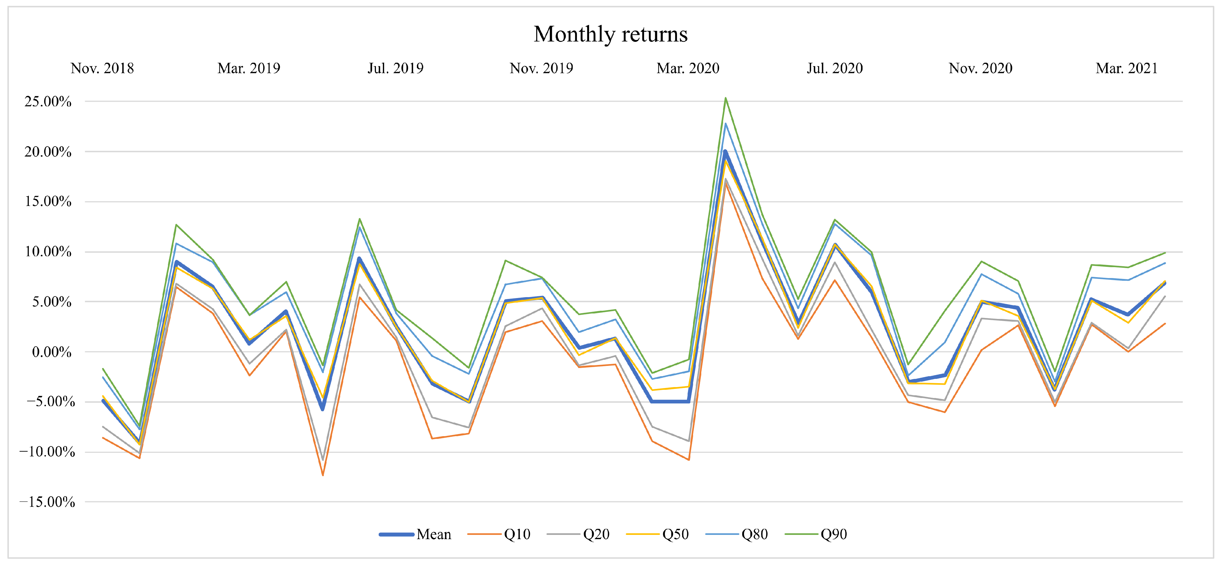
The proposed approach uses components that exploit randomness to explore the search space. Here, we intend to discard the effects produced by such randomness by running our approach many times; particularly, each stochastic component runs twenty times for each of the thirty back-testing periods mentioned in Section 5.1. Doing it this way sheds light on the robustness of our approach and allows us to reach sound conclusions. By following the recommendations in [88], the performance of our approach is evaluated by using the quantiles $Q_{10}$, $Q_{20}$, $Q_{50}$ (median), $Q_{80}$ and $Q_{90}$ (see Figure 1). As is noted in [88], distribution solutions of stochastic optimization algorithms are often asymmetrical; hence by using quantiles, we could obtain more insights into our approaches. However, Figure 1 shows that, in our case, $Q_{50}$ and the mean are almost always overlapped. Furthermore, ($Q_{10}$, $Q_{20}$) and ($Q_{80}$, $Q_{90}$) are symmetrical with respect to the mean. This behavior indicate that the performance of our approach is practically normally distributed.

Therefore, in this study, the average returns of our approach is used to be compared with several benchmarks, as shown in

Table 1. Returns produced per period. In the case of the algorithms, the return is averaged in twenty runs.

	S&P500 Index	Yang et al. (2019)	Solares et al. (2019)	Without Negative Trends	With Negative Trends
Nov. 2018	1.75%	1.01%	1.87%	−5.11%	−4.87%
Dec. 2018	−10.11%	−9.18%	−8.81%	−9.56%	−9.14%
Jan. 2019	7.29%	10.88%	6.71%	6.77%	9.00%
Feb. 2019	2.89%	7.47%	4.19%	7.00%	6.52%
Mar. 2019	1.76%	0.20%	2.17%	0.89%	0.81%
Apr. 2019	3.78%	4.29%	4.65%	3.88%	4.06%
May. 2019	−7.04%	−7.22%	−5.65%	−7.66%	−5.77%
Jun. 2019	6.45%	8.45%	7.53%	8.06%	9.33%
Jul. 2019	1.30%	0.25%	0.92%	2.66%	2.64%
Aug. 2019	−1.84%	−1.08%	−1.78%	−0.03%	−3.19%
Sep. 2019	1.69%	−1.63%	0.83%	−6.20%	−4.96%
Oct. 2019	2.00%	3.12%	1.67%	5.85%	5.09%
Nov. 2019	3.29%	2.58%	4.00%	4.17%	5.43%
Dec. 2019	2.78%	1.13%	2.39%	0.13%	0.36%
Jan. 2020	−0.16%	0.81%	1.67%	2.13%	1.29%
Feb. 2020	−9.18%	−9.09%	−9.28%	−7.22%	−4.96%
Mar. 2020	−14.30%	−10.27%	−14.03%	−6.59%	−4.94%
Apr. 2020	11.26%	14.33%	12.53%	19.64%	20.02%
May. 2020	4.33%	7.09%	7.02%	11.54%	11.11%
Jun. 2020	1.81%	−0.29%	0.15%	1.95%	2.88%
Jul. 2020	5.22%	4.18%	5.87%	5.28%	10.65%
Aug. 2020	6.55%	4.68%	3.90%	4.18%	5.94%
Sep. 2020	−4.08%	−3.95%	−1.10%	−3.20%	−3.04%
Oct. 2020	−2.85%	−4.74%	−2.05%	−5.88%	−2.31%
Nov. 2020	9.71%	11.50%	11.91%	8.28%	4.97%
Dec. 2020	3.58%	2.95%	5.39%	3.33%	4.37%
Jan. 2021	−1.13%	−2.23%	−0.53%	−3.06%	−3.76%
Feb. 2021	2.54%	3.43%	8.35%	1.51%	5.23%
Mar. 2021	4.07%	7.22%	3.23%	0.88%	3.75%
Apr. 2021	4.98%	6.05%	5.09%	6.00%	6.84%
Average	1.28%	1.73%	1.96%	1.65%	2.45%
Std desv.	5.61%	6.06%	5.76%	6.35%	6.27%

and Figure 2. For simplicity, the results are discussed hereafter as if the returns were not averages. In order to validate our approach, in this section, we have included several benchmarks to measure the effectiveness of our proposal. These benchmarks are: (a) the market index S&P500, (b) the approach of [10], (c) the approach of [12] and (d) our approach without including downtrends.

From Table 1 and Figure 2, we can see that, in terms of the expected value, the worst overall return was produced by investing according to the S&P500 index, while the best overall return was achieved by investing in a portfolio produced by the proposed approach that takes advantage of both positive and negative trends. Figure 2 shows that the portfolio that considers negative trends is almost always in the top two from all the approaches. Furthermore, the returns obtained using this approach show that this model is not affected by the downtrends in the market as the benchmarks, as seen in the fall of all approaches from Jan 2020 to Mar 2020. Remarkably, this behavior did not prevent the proposed approach from exploiting the clear overall uptrend produced from Apr. 2020 to Apr. 2021, as can be clearly seen in Table 1.

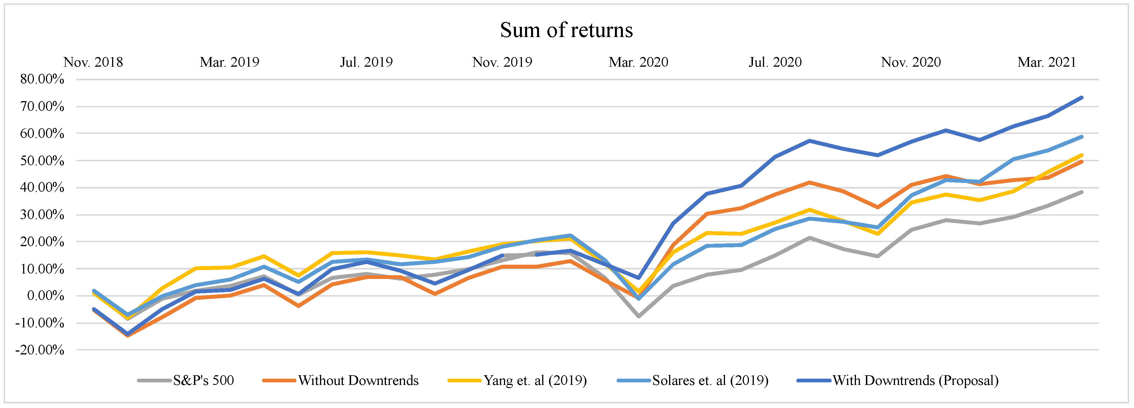
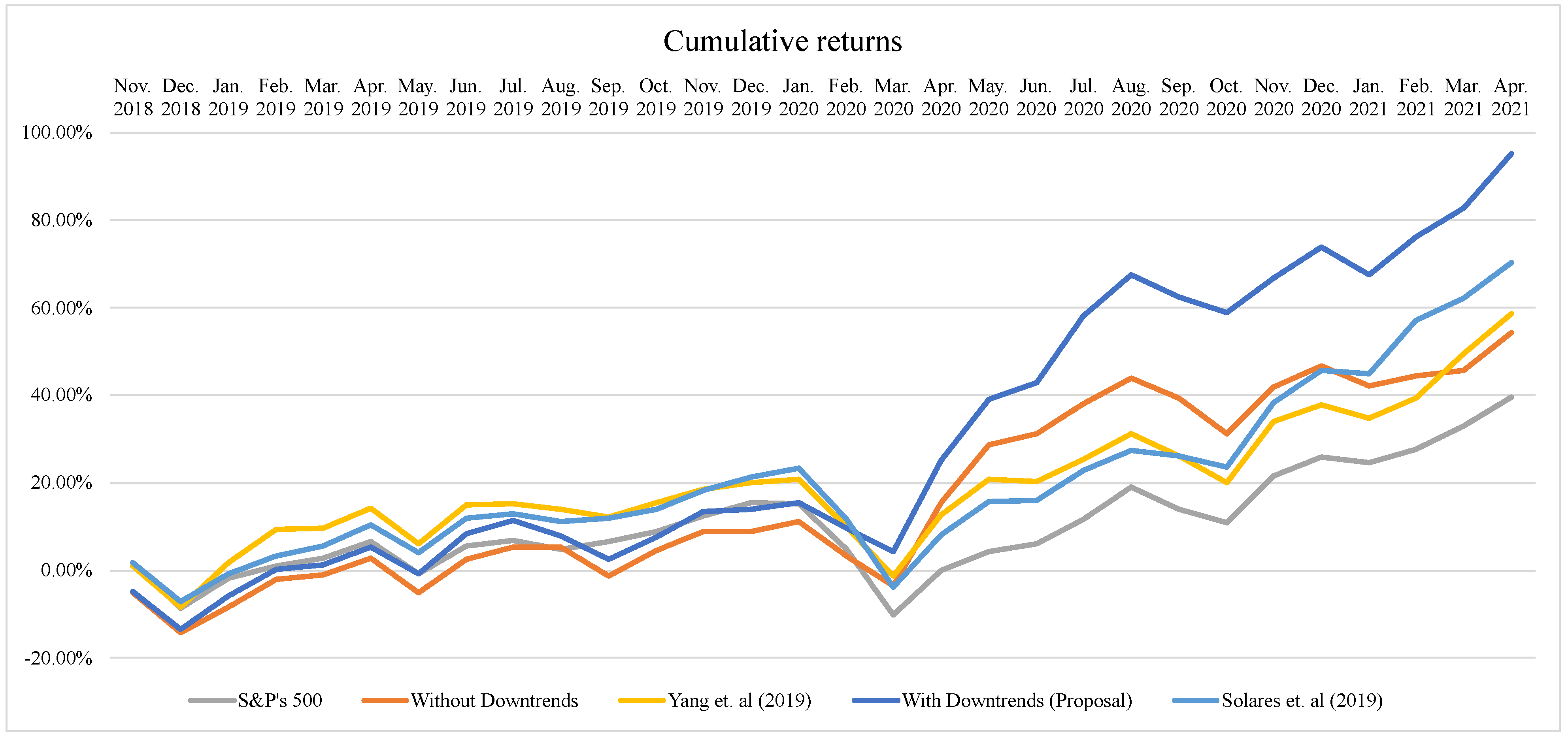
From

Table 2. Sum of returns and cumulative returns. In the case of the algorithms, the return is averaged over twenty runs.

	Sum of Returns					Cumulative Returns
	S&P500 Index	Yang et al. (2019)	Solares et al. (2019)	Without Down- Trends	With Down- Trends	S&P500 Index	Yang et al. (2019)	Solares et al. (2019)	Without Down- Trends	With Down- Trends
Nov. 2018	1.75%	1.01%	1.87%	−5.11%	−4.87%	1.75%	1.01%	1.87%	−5.11%	−4.87%
Dec. 2018	−8.35%	−8.17%	−6.94%	−14.67%	−14.01%	−8.53%	−8.27%	−7.11%	−14.18%	−13.56%
Jan. 2019	−1.06%	2.70%	−0.24%	−7.89%	−5.01%	−1.86%	1.71%	−0.88%	−8.37%	−5.79%
Feb. 2019	1.83%	10.17%	3.95%	−0.89%	1.51%	0.98%	9.31%	3.28%	−1.95%	0.36%
Mar. 2019	3.59%	10.37%	6.12%	0.00%	2.32%	2.76%	9.53%	5.52%	−1.08%	1.17%
Apr. 2019	7.37%	14.66%	10.77%	3.88%	6.38%	6.64%	14.23%	10.42%	2.76%	5.28%
May. 2019	0.33%	7.44%	5.12%	−3.78%	0.61%	−0.87%	5.98%	4.18%	−5.11%	−0.80%
Jun. 2019	6.78%	15.89%	12.65%	4.28%	9.94%	5.53%	14.93%	12.03%	2.54%	8.46%
Jul. 2019	8.08%	16.14%	13.58%	6.94%	12.58%	6.89%	15.22%	13.07%	5.27%	11.32%
Aug. 2019	6.24%	15.06%	11.80%	6.91%	9.39%	4.93%	13.97%	11.05%	5.23%	7.77%
Sep. 2019	7.92%	13.43%	12.63%	0.70%	4.43%	6.70%	12.11%	11.98%	−1.29%	2.43%
Oct. 2019	9.93%	16.54%	14.30%	6.56%	9.52%	8.83%	15.61%	13.85%	4.48%	7.64%
Nov. 2019	13.22%	19.12%	18.30%	10.72%	14.95%	12.42%	18.59%	18.40%	8.84%	13.48%
Dec. 2019	16.00%	20.25%	20.68%	10.85%	15.31%	15.54%	19.93%	21.22%	8.97%	13.89%
Jan. 2020	15.84%	21.06%	22.36%	12.98%	16.60%	15.35%	20.90%	23.25%	11.30%	15.36%
Feb. 2020	6.65%	11.98%	13.07%	5.76%	11.64%	4.76%	9.92%	11.81%	3.26%	9.64%
Mar. 2020	−7.65%	1.71%	−0.96%	−0.83%	6.70%	−10.22%	−1.37%	−3.88%	−3.54%	4.23%
Apr. 2020	3.61%	16.04%	11.57%	18.81%	26.73%	−0.12%	12.77%	8.16%	15.40%	25.10%
May. 2020	7.94%	23.13%	18.58%	30.36%	37.84%	4.21%	20.76%	15.75%	28.72%	38.99%
Jun. 2020	9.75%	22.84%	18.73%	32.31%	40.72%	6.09%	20.41%	15.91%	31.24%	43.00%
Jul. 2020	14.97%	27.01%	24.60%	37.59%	51.37%	11.63%	25.43%	22.72%	38.16%	58.23%
Aug. 2020	21.52%	31.69%	28.51%	41.77%	57.31%	18.94%	31.30%	27.51%	43.94%	67.63%
Sep. 2020	17.43%	27.74%	27.41%	38.57%	54.28%	14.09%	26.12%	26.11%	39.33%	62.54%
Oct. 2020	14.59%	23.01%	25.36%	32.68%	51.97%	10.84%	20.14%	23.53%	31.13%	58.80%
Nov. 2020	24.30%	34.51%	37.27%	40.97%	56.94%	21.60%	33.97%	38.24%	41.99%	66.69%
Dec. 2020	27.88%	37.47%	42.66%	44.30%	61.31%	25.96%	37.92%	45.70%	46.73%	73.97%
Jan. 2021	26.75%	35.23%	42.14%	41.24%	57.55%	24.54%	34.85%	44.93%	42.24%	67.43%
Feb. 2021	29.29%	38.66%	50.48%	42.75%	62.78%	27.70%	39.47%	57.03%	44.39%	76.18%
Mar. 2021	33.36%	45.88%	53.71%	43.63%	66.52%	32.90%	49.54%	62.10%	45.66%	82.78%
Apr. 2021	38.35%	51.93%	58.80%	49.64%	73.36%	39.52%	58.59%	70.35%	54.41%	95.28%

, we can see that the proposed approach outperforms the benchmarks at the end of the thirty periods: the sum of returns is approximately 41% better than Yang et al. 2019 ([10]), 25% better than Solares et al. 2019 ([12]), 48% better than the one that only considers positive trends and more than 90% better than the market index. Moreover, the cumulative returns of our proposal is 63% better than Yang et al. 2019 ([10]), 35% better than Solares et al. 2019 ([12]), 75% better than the one that only considers positive trends and 141% better than the market index. This performance can be seen in Figure 3 and Figure 4.

Both Figure 3 and Figure 4 describe the evolution of the portfolio returns in an aggregate way throughout the whole time lapse (i.e., November 2018 to April 2021). However, Figure 3 shows this evolution from the perspective of the sums of the returns, while Figure 4 shows the cumulative returns. Both figures can be relevant to the practitioner. The former shows the overall performance of the approach without considering the exact period where the return was obtained, while Figure 4 allows one to ponder the impact of the period where such a return was obtained. Let us unfold the latter. Figure 4 shows the amount that the investor would obtain if he/she takes their investment in a given period. For instance, an investment of USD 1000 at the beginning of November 2018 using the proposed model would have become USD 992 (i.e., −0.80%) if the investor would have withdrawn the investment at the end of May 2019. However, if he/she continues until April 2021, the investment would have become USD 1952 (i.e., +95.28%). In this sense, it is clear that the proposed approach outperformed the benchmarks by creating a portfolio that includes long and short positions. This result shows the potential of our proposal, which could be improved in future approaches by including stocks from other indexes, more technical/fundamental variables, etc.

In both Figures, it can be seen that, for the first fourteen periods (November 2018 to December 2019), the market does not move significantly in any direction; however, for the remaining periods, the market starts both negative and positive trends. A higher final return achieved by our proposal indicates that it is taking advantage of these trends overall. These results also show that considering negative trends is crucial. The figures show that the final average return is better if negative trends are considered when building stock portfolios.

According to Figure 2 and Table 1, the worst return obtained by our approach was in Dec 2018. This is also shown in Figure 4, where the detriment is caused by the higher negative return produced in this period. In that moment, the system decided to open long positions and allocate high proportions of investments to some stocks with bad actual returns. This was due to the good historical performance of such actions that indicated a good statistical behavior. Several external issues affect the performance of a stock in the market, such as the case of Nvidia corporation as reported in the news [89]. Thus, a way of improving the proposed system in the future is by considering criteria coming from the so-called sentiment analysis [90] that takes into consideration such factors.

On the other hand, as a way of measuring the performance of our proposal and comparing the results with some benchmarks, the Sharpe ratio $r_{sharpe}$ and Sortino ratio $r_{sortino}$ are used. These ratios are defined as

$$\begin{array}{c}\hfill r_{sharpe}=\frac{R_p-R_f}{{\sigma }_p}\end{array}$$

and

$$\begin{array}{c}\hfill r_{sortino}=\frac{R_p-R_f}{{\sigma }_{pd}}\end{array}$$

where $R_p$ is the average portfolio return, $R_f$ is the best available risk-free security rate, ${\sigma }_p$ is the portfolio standard deviation and ${\sigma }_{p,d}$ is the portfolio standard deviation of the downside. These indexes measure the risk per return obtained in comparison with a risk-free asset. In particular, the Sharpe ratio describes how much return is received per unit of risk; meanwhile, the Sortino ratio describes how much return is received per unit of bad risk. Therefore, the higher these indexes are, the more convenient for investment the asset is. We have considered the Treasure Bond of USA a risk-free security, with a value of 3% of annual return. We also considered the Treasure Bond of USA as the minimal acceptance ratio (MAR) to compute the downside deviation. $R_p$, ${\sigma }_p$ and ${\sigma }_{p,d}$ are taken from Table 1.

Table 3. Comparison of benchmarks with the proposal by using the Sharpe and Sortino ratios.

	Sharpe Ratio	Sortino Ratio
S&P’s 500	0.1831	0.2529
Yang et al. (2019)	0.2445	0.4072
Solares et al. (2019)	0.2966	0.4551
Without downtrends	0.2213	0.3884
With downtrends	0.3502	0.7223

shows the Sharpe and Sortino ratios for the all the benchmarks and our proposal. According to the results, our proposal has the best performance for both indexes; overall, it has higher returns by considering the risk.

6. Conclusions

Building stock portfolios with high returns and low risk is a common challenge for researchers in the financial area. Usually, the most common practice is to select the more promising stocks according to several factors, such as financial information, news of the market and technical analysis. Several approaches that use computational intelligence algorithms have been proposed in the literature to deal with the overwhelming complexity of building a stock portfolio. Usually, these approaches consider up to three activities to build a portfolio: return forecasting, stock selection and portfolio optimization. These activities decide which stocks should be supported, as well as the proportions of the investment to be allocated to them, by comparing the historical and forecasted performance of potential stock investments. However, to the best of our knowledge, these approaches do not comprehensively address the three activities when considering downtrends in stock prices.

In this paper, a comprehensive approach to stock portfolio management is proposed; the approach includes stock price forecasting, stock selection and stock portfolio optimization while taking advantage of market downtrends.

Stock price forecasting is carried out through an artificial neural network (ANN) trained by the extreme learning machine (ELM) algorithm. Forecasting the price of a given stock allows the comprehensive approach to focus on uptrends or downtrends (i.e., going long or short, respectively) for that stock. Stock selection is modeled as an optimization problem that seeks to determine the most plausible stocks; thus, a differential evolution is exploited on the basis of the forecasted price and a set of factors of the so-called fundamental analysis. Finally, portfolio optimization is conducted through a genetic algorithm that uses confidence intervals of the portfolio returns to determine the best stock portfolio.

Using preliminary experimentation, we found that the ELM was better than other methods (ANN with back-propagation, random forest, support vector regression) at forecasting the trend of the stock price but not the best at forecasting stock returns. Therefore, more research should be conducted to discover better configurations of the ANN with ELM or to decide if the forecasting stage should be changed. However, further research on this, as well as on methods to increase the performance of the next stages of the comprehensive approach, is beyond the scope of this work, so the authors will address these issues in future works.

Regarding the assessment of the comprehensive approach, the obtained results show that stock selection and portfolio optimization stages make more profitable portfolios when negative trends of stocks are taken into account to take advantage of downtrends of the market (see Table 2 and Figure 3 and Figure 4). Furthermore, the results show that not only a traditional benchmark, the Standard and Poor’s 500 index, is outperformed by the proposed approach but also approaches that do not exploit negative market trends (e.g., [10,12]).

This research work could be improved by the following possible future directions:

I

A deeper study of the forecasting stage to test the performance of several AI methods by employing more data or different financial variables;

II

A deeper study on the selection stage to evaluate the performance of the system by employing different financial variables to build the stock portfolio;

III

A deeper study of the performance of the system by modifying different parameters in the optimization stage and comparing the results with other approaches;

IV

New experiments to show the robustness of the approach regarding (i) the number and type of alternatives in the universe of stocks, (ii) the number of selected stocks and (iii) the parameter values.

References

- Pan, H.; Long, M. Intelligent Portfolio Theory and Application in Stock Investment with Multi-Factor Models and Trend Following Trading Strategies. Procedia Comput. Sci. 2021, 187, 414–419. [Google Scholar] [CrossRef]
- Jiang, X.; Peterburgsky, S. Investment performance of shorted leveraged ETF pairs. Appl. Econ. 2017, 49, 4410–4427. [Google Scholar] [CrossRef]
- Hurlin, C.; Iseli, G.; Pérignon, C.; Yeung, S. The counterparty risk exposure of ETF investors. J. Bank. Financ. 2019, 102, 215–230. [Google Scholar] [CrossRef]
- Holzhauer, H.M.; Lu, X.; McLeod, R.W.; Mehran, J. Bad news bears: Effects of expected market volatility on daily tracking error of leveraged bull and bear ETFs. Manag. Financ. 2013, 39, 1169–1187. [Google Scholar]
- Gregory-Allen, R.B.; Smith, D.M.; Werman, M. Chapter 30—Short Selling by Portfolio Managers: Performance and Risk Effects across Investment Styles. In Handbook of Short Selling; Gregoriou, G.N., Ed.; Academic Press: San Diego, CA, USA, 2012; pp. 437–451. [Google Scholar] [CrossRef]
- Huang, G.B.; Zhu, Q.Y.; Siew, C.K. Extreme learning machine: Theory and applications. Neurocomputing 2006, 70, 489–501. [Google Scholar] [CrossRef]
- Li, X.; Xie, H.; Wang, R.; Cai, Y.; Cao, J.; Wang, F.; Min, H.; Deng, X. Empirical analysis: Stock market prediction via extreme learning machine. Neural Comput. Appl. 2016, 27, 67–78. [Google Scholar] [CrossRef]
- Wang, F.; Zhang, Y.; Rao, Q.; Li, K.; Zhang, H. Exploring mutual information-based sentimental analysis with kernel-based extreme learning machine for stock prediction. Soft Comput. 2017, 21, 3193–3205. [Google Scholar] [CrossRef]
- Das, S.P.; Padhy, S. Unsupervised extreme learning machine and support vector regression hybrid model for predicting energy commodity futures index. Memetic Comput. 2017, 9, 333–346. [Google Scholar] [CrossRef]
- Yang, F.; Chen, Z.; Li, J.; Tang, L. A novel hybrid stock selection method with stock prediction. Appl. Soft Comput. 2019, 80, 820–831. [Google Scholar] [CrossRef]
- Fernandez, E.; Navarro, J.; Solares, E.; Coello, C.C. A novel approach to select the best portfolio considering the preferences of the decision maker. Swarm Evol. Comput. 2019, 46, 140–153. [Google Scholar] [CrossRef]
- Solares, E.; Coello, C.A.C.; Fernandez, E.; Navarro, J. Handling uncertainty through confidence intervals in portfolio optimization. Swarm Evol. Comput. 2019, 44, 774–787. [Google Scholar] [CrossRef]
- Xidonas, P.; Mavrotas, G.; Psarras, J. A multicriteria methodology for equity selection using financial analysis. Comput. Oper. Res. 2009, 36, 3187–3203. [Google Scholar] [CrossRef]
- Marasović, B.; Poklepović, T.; Aljinović, Z. MArkowitz’model with fundamental and technical analysis–complementary methods or not. Croat. Oper. Res. Rev. 2011, 2, 122–132. [Google Scholar]
- Abiodun, O.I.; Jantan, A.; Omolara, A.E.; Dada, K.V.; Mohamed, N.A.; Arshad, H. State-of-the-art in artificial neural network applications: A survey. Heliyon 2018, 4, e00938. [Google Scholar] [CrossRef] [PubMed] [Green Version]
- Sumathi, S.; Paneerselvam, S. Computational Intelligence Paradigms: Theory & Applications Using MATLAB; CRC Press: New York, NY, USA, 2010. [Google Scholar]
- Albawi, S.; Mohammed, T.A.; Al-Zawi, S. Understanding of a convolutional neural network. In Proceedings of the 2017 International Conference on Engineering and Technology (ICET), Antalya, Turkey, 21–23 August 2017; pp. 1–6. [Google Scholar]
- Coello, C.A.C.; Lamont, G.B.; Van Veldhuizen, D.A. Evolutionary Algorithms for Solving Multi-Objective Problems; Springer: Berlin, Germany, 2007; Volume 5. [Google Scholar]
- Bianchi, L.; Dorigo, M.; Gambardella, L.M.; Gutjahr, W.J. A survey on metaheuristics for stochastic combinatorial optimization. Nat. Comput. 2009, 8, 239–287. [Google Scholar] [CrossRef] [Green Version]
- Pławiak, P. Novel genetic ensembles of classifiers applied to myocardium dysfunction recognition based on ECG signals. Swarm Evol. Comput. 2018, 39, 192–208. [Google Scholar] [CrossRef]
- Pławiak, P. Novel methodology of cardiac health recognition based on ECG signals and evolutionary-neural system. Expert Syst. Appl. 2018, 92, 334–349. [Google Scholar] [CrossRef]
- Das, S.; Suganthan, P.N. Differential evolution: A survey of the state-of-the-art. IEEE Trans. Evol. Comput. 2010, 15, 4–31. [Google Scholar] [CrossRef]
- Krink, T.; Paterlini, S. Multiobjective optimization using differential evolution for real-world portfolio optimization. Comput. Manag. Sci. 2011, 8, 157–179. [Google Scholar] [CrossRef]
- Krink, T.; Mittnik, S.; Paterlini, S. Differential evolution and combinatorial search for constrained index-tracking. Ann. Oper. Res. 2009, 172, 153. [Google Scholar] [CrossRef]
- Zhang, Q.; Li, H. MOEA/D: A Multiobjective Evolutionary Algorithm Based on Decomposition. IEEE Trans. Evol. Comput. 2007, 11, 712–731. [Google Scholar] [CrossRef]
- Sharma, D.K.; Hota, H.; Brown, K.; Handa, R. Integration of genetic algorithm with artificial neural network for stock market forecasting. Int. J. Syst. Assur. Eng. Manag. 2021, 1–14. [Google Scholar] [CrossRef]
- Ferreira, F.; Gandomi, A.H.; Cardoso, R.T.N. Artificial Intelligence Applied to Stock Market Trading: A Review. IEEE Access 2021, 9, 30898–30917. [Google Scholar] [CrossRef]
- Chopra, R.; Sharma, G.D. Application of Artificial Intelligence in Stock Market Forecasting: A Critique, Review, and Research Agenda. J. Risk Financ. Manag. 2021, 14, 526. [Google Scholar] [CrossRef]
- Ma, Y.L.; Han, R.Z.; Wang, W.Z. Prediction-Based Portfolio Optimization Models Using Deep Neural Networks. IEEE Access 2020, 8, 115393–115405. [Google Scholar] [CrossRef]
- Fischer, T.; Krauss, C. Deep learning with long short-term memory networks for financial market predictions. Eur. J. Oper. Res. 2018, 270, 654–669. [Google Scholar] [CrossRef] [Green Version]
- Long, W.; Lu, Z.; Cui, L. Deep learning-based feature engineering for stock price movement prediction. Knowl.-Based Syst. 2019, 164, 163–173. [Google Scholar] [CrossRef]
- Zhong, X.; Enke, D. Predicting the daily return direction of the stock market using hybrid machine learning algorithms. Financ. Innov. 2019, 5, 1–20. [Google Scholar] [CrossRef]
- Kaczmarek, T.; Perez, K. Building portfolios based on machine learning predictions. Econ. Res.-Ekon. Istraz. 2021, 1–19. [Google Scholar] [CrossRef]
- Patel, J.; Shah, S.; Thakkar, P.; Kotecha, K. Predicting stock and stock price index movement using Trend Deterministic Data Preparation and machine learning techniques. Expert Syst. Appl. 2015, 42, 259–268. [Google Scholar] [CrossRef]
- Chong, E.; Han, C.; Park, F.C. Deep learning networks for stock market analysis and prediction: Methodology, data representations, and case studies. Expert Syst. Appl. 2017, 83, 187–205. [Google Scholar] [CrossRef] [Green Version]
- Huang, G.B.; Siew, C.K. Extreme learning machine: RBF network case. In Proceedings of the 2004 8th International Conference on Control, Automation, Robotics and Vision (ICARCV) ICARCV 2004, Kunming, China, 6–9 December 2004; Volume 2, pp. 1029–1036. [Google Scholar] [CrossRef]
- Peykani, P.; Mohammadi, E.; Jabbarzadeh, A.; Rostamy-Malkhalifeh, M.; Pishvaee, M.S. A novel two-phase robust portfolio selection and optimization approach under uncertainty: A case study of Tehran stock exchange. PLoS ONE 2020, 15, e239810. [Google Scholar] [CrossRef] [PubMed]
- Mussafi, N.S.M.; Ismail, Z. Optimum Risk-Adjusted Islamic Stock Portfolio Using the Quadratic Programming Model: An Empirical Study in Indonesia. J. Asian Financ. Econ. Bus. 2021, 8, 839–850. [Google Scholar] [CrossRef]
- Lim, S.; Kim, M.J.; Ahn, C.W. A Genetic Algorithm (GA) Approach to the Portfolio Design Based on Market Movements and Asset Valuations. IEEE Access 2020, 8, 140234–140249. [Google Scholar] [CrossRef]
- Wang, W.Y.; Li, W.Z.; Zhang, N.; Liu, K.C. Portfolio formation with preselection using deep learning from long-term financial data. Expert Syst. Appl. 2020, 143, 113042. [Google Scholar] [CrossRef]
- Zhang, C.; Liang, S.; Lyu, F.; Fang, L. Stock-index tracking optimization using auto-encoders. Front. Phys. 2020, 8, 388. [Google Scholar] [CrossRef]
- Paiva, F.D.; Cardoso, R.T.N.; Hanaoka, G.P.; Duarte, W.M. Decision-making for financial trading: A fusion approach of machine learning and portfolio selection. Expert Syst. Appl. 2019, 115, 635–655. [Google Scholar] [CrossRef]
- Galankashi, M.R.; Rafiei, F.M.; Ghezelbash, M. Portfolio selection: A fuzzy-ANP approach. Financ. Innov. 2020, 6, 34. [Google Scholar] [CrossRef]
- Markowitz, H. Portfolio Selection. J. Financ. 1952, 7, 77–91. [Google Scholar]
- Kalayci, C.B.; Ertenlice, O.; Akbay, M.A. A comprehensive review of deterministic models and applications for mean-variance portfolio optimization. Expert Syst. Appl. 2019, 125, 345–368. [Google Scholar] [CrossRef]
- Rockafellar, R.; Uryasev, S. Optimization of conditional value-at-risk. J. Risk 2002, 2, 21–41. [Google Scholar] [CrossRef] [Green Version]
- Rockafellar, R.; Uryasev, S. Conditional value-at-risk for general loss distributions. J. Bank. Financ. 2002, 26, 1443–1471. [Google Scholar] [CrossRef]
- Sehgal, R.; Mehra, A. Robust reward–risk ratio portfolio optimization. Int. Trans. Oper. Res. 2021, 28, 2169–2190. [Google Scholar] [CrossRef]
- Hu, Y.; Lindquist, W.B.; Rachev, S.T. Portfolio Optimization Constrained by Performance Attribution. J. Risk Financ. Manag. 2021, 14, 201. [Google Scholar] [CrossRef]
- Dai, Z.; Wen, F. Some improved sparse and stable portfolio optimization problems. Financ. Res. Lett. 2018, 27, 46–52. [Google Scholar] [CrossRef]
- Baykasoğlu, A.; Yunusoglu, M.G.; Özsoydan, F.B. A GRASP based solution approach to solve cardinality constrained portfolio optimization problems. Comput. Ind. Eng. 2015, 90, 339–351. [Google Scholar] [CrossRef]
- Mayambala, F.; Rönnberg, E.; Larsson, T. Eigendecomposition of the Mean-Variance Portfolio Optimization Model. In Optimization, Control, and Applications in the Information Age; Migdalas, A., Karakitsiou, A., Eds.; Springer International Publishing: Cham, Switzerland, 2015; pp. 209–232. [Google Scholar]
- Kocadağli, O.; Keskin, R. A novel portfolio selection model based on fuzzy goal programming with different importance and priorities. Expert Syst. Appl. 2015, 42, 6898–6912. [Google Scholar] [CrossRef]
- He, F.; Qu, R. Hybridising Local Search With Branch-And-Bound For Constrained Portfolio Selection Problems. In Proceedings of the 30th European Council for Modeling and Simulation, Regensburg, Germany, 31 May–3 June 2016; Claus, T., Herrmann, F., Manitz, M., Rose, O., Eds.; Digital Library of the European Council for Modelling and Simulation: Regensburg, Germany, 2016; pp. 1–7. [Google Scholar]
- Ruiz-Torrubiano, R.; Suárez, A. A memetic algorithm for cardinality-constrained portfolio optimization with transaction costs. Appl. Soft Comput. 2015, 36, 125–142. [Google Scholar] [CrossRef] [Green Version]
- Soleymani, F.; Paquet, E. Financial portfolio optimization with online deep reinforcement learning and restricted stacked autoencoder—DeepBreath. Expert Syst. Appl. 2020, 156, 113456. [Google Scholar] [CrossRef]
- García, F.; Guijarro, F.; Oliver, J. Index tracking optimization with cardinality constraint: A performance comparison of genetic algorithms and tabu search heuristics. Neural Comput. Appl. 2018, 30, 2625–2641. [Google Scholar] [CrossRef]
- Hadi, A.S.; Naggar, A.A.E.; Bary, M.N.A. New model and method for portfolios selection. Appl. Math. Sci. 2016, 10, 263–288. [Google Scholar] [CrossRef]
- Liagkouras, K.; Metaxiotis, K. A new efficiently encoded multiobjective algorithm for the solution of the cardinality constrained portfolio optimization problem. Ann. Oper. Res. 2018, 267, 281–319. [Google Scholar] [CrossRef]
- Macedo, L.L.; Godinho, P.; Alves, M.J. Mean-semivariance portfolio optimization with multiobjective evolutionary algorithms and technical analysis rules. Expert Syst. Appl. 2017, 79, 33–43. [Google Scholar] [CrossRef]
- Lwin, K.T.; Qu, R.; MacCarthy, B.L. Mean-VaR portfolio optimization: A nonparametric approach. Eur. J. Oper. Res. 2017, 260, 751–766. [Google Scholar] [CrossRef] [Green Version]
- Ban, G.Y.; Karoui, N.E.; Lim, A.E.B. Machine Learning and Portfolio Optimization. Manag. Sci. 2016, 64, 1136–1154. [Google Scholar] [CrossRef] [Green Version]
- Kizys, R.; Juan, A.; Sawik, B.; Calvet, L. A Biased-Randomized Iterated Local Search Algorithm for Rich Portfolio Optimization. Appl. Sci. 2019, 9, 3509. [Google Scholar] [CrossRef] [Green Version]
- Kalayci, C.B.; Ertenlice, O.; Akyer, H.; Aygoren, H. An artificial bee colony algorithm with feasibility enforcement and infeasibility toleration procedures for cardinality constrained portfolio optimization. Expert Syst. Appl. 2017, 85, 61–75. [Google Scholar] [CrossRef]
- Mendonça, G.H.; Ferreira, F.G.; Cardoso, R.T.; Martins, F.V. Multi-attribute decision making applied to financial portfolio optimization problem. Expert Syst. Appl. 2020, 158, 113527. [Google Scholar] [CrossRef]
- Fernández, E.; Figueira, J.R.; Navarro, J. An interval extension of the outranking approach and its application to multiple-criteria ordinal classification. Omega 2019, 84, 189–198. [Google Scholar] [CrossRef]
- Sunaga, T. Theory of an Interval Algebra and Its Applications to Numerical Analysis. RAAG Memoirs 1958, 2, 29–46. [Google Scholar] [CrossRef]
- Moore, R.E. Interval Arithmetic And Automatic Error Analysis in Digital Computing; Stanford University: Stanford, CA, USA, 1963. [Google Scholar]
- Hui, E.C.; Chan, K.K.K. Alternative trading strategies to beat “buy-and-hold”. Phys. A Stat. Mech. Its Appl. 2019, 534, 120800. [Google Scholar] [CrossRef]
- Hui, E.C.; Chan, K.K.K. A new time-dependent trading strategy for securitized real estate and equity indices. Int. J. Strateg. Prop. Manag. 2018, 22, 64–79. [Google Scholar] [CrossRef] [Green Version]
- Allen, D.E.; Powell, R.J.; Singh, A.K. Chapter 32—Machine Learning and Short Positions in Stock Trading Strategies. In Handbook of Short Selling; Gregoriou, G.N., Ed.; Academic Press: San Diego, CA, USA, 2012; pp. 467–478. [Google Scholar] [CrossRef]
- Baumann, M.H.; Grüne, L. Simultaneously long-short trading in discrete and continuous time. Syst. Control. Lett. 2017, 99, 85–89. [Google Scholar] [CrossRef] [Green Version]
- Primbs, J.A.; Barmish, B.R. On Robustness of Simultaneous Long-Short Stock Trading Control with Time-Varying Price Dynamics. IFAC-PapersOnLine 2017, 50, 12267–12272. [Google Scholar] [CrossRef]
- O’Brien, J.D.; Burke, M.E.; Burke, K. A Generalized Framework for Simultaneous Long-Short Feedback Trading. IEEE Trans. Autom. Control. 2021, 66, 2652–2663. [Google Scholar] [CrossRef]
- Deshpande, A.; Gubner, J.A.; Barmish, B.R. On Simultaneous Long-Short Stock Trading Controllers with Cross-Coupling. IFAC PapersOnLine 2020, 53, 16989–16995. [Google Scholar] [CrossRef]
- Fu, X.; Du, J.; Guo, Y.; Liu, M.; Dong, T.; Duan, X. A machine learning framework for stock selection. arXiv 2018, arXiv:1806.01743. [Google Scholar]
- Zhang, R.; Lin, Z.; Chen, S.; Lin, Z.; Liang, X. Multi-factor Stock Selection Model Based on Kernel Support Vector Machine. J. Math. Res 2018, 10, 9. [Google Scholar] [CrossRef]
- Becker, Y.L.; Fei, P.; Lester, A.M. Stock selection: An innovative application of genetic programming methodology. In Genetic Programming Theory and Practice IV; Springer: Berlin, Germany, 2007; pp. 315–334. [Google Scholar]
- Levin, A. Stock selection via nonlinear multi-factor models. Adv. Neural Inf. Process. Syst. 1995, 8, 966–972. [Google Scholar]
- Storn, R.; Price, K. Differential evolution—A simple and efficient heuristic for global optimization over continuous spaces. J. Glob. Optim. 1997, 11, 341–359. [Google Scholar] [CrossRef]
- Sengupta, A.; Pal, T.K. On comparing interval numbers. Eur. J. Oper. Res. 2000, 127, 28–43. [Google Scholar] [CrossRef]
- Ishibuchi, H.; Tanaka, H. Multiobjective programming in optimization of the interval objective function. Eur. J. Oper. Res. 1990, 48, 219–225. [Google Scholar] [CrossRef]
- Shi, J.R.; Liu, S.Y.; Xiong, W.T. A new solution for interval number linear programming. Syst. Eng.-Theory Pract. 2005, 2, 16. [Google Scholar]
- Solares, E.; Fernandez, E.; Navarro, J. A generalization of the outranking approach by incorporating uncertainty as interval numbers. Investig. Oper. 2019, 39, 501–514. [Google Scholar]
- Li, G.-D.; Yamaguchi, D.; Nagai, M. A grey-based decision-making approach to the supplier selection problem. Math. Comput. Model. 2007, 46, 573–581. [Google Scholar] [CrossRef]
- Bhattacharyya, R. A grey theory based multiple attribute approach for r&d project portfolio selection. Fuzzy Inf. Eng. 2015, 7, 211–225. [Google Scholar]
- Fernández, E.; Navarro, J.; Solares, E. A hierarchical interval outranking approach with interacting criteria. Eur. J. Oper. Res. 2022, 298, 293–307. [Google Scholar] [CrossRef]
- Ivkovic, N.; Jakobovic, D.; Golub, M. Measuring Performance of Optimization Algorithms in Evolutionary Computation. Int. J. Mach. Learn. Comput. 2016, 6, 167–171. [Google Scholar] [CrossRef]
- McKenna, B. Why NVIDIA Stock Plunged 31% in 2018; Motley Fool: Alexandria, VA, USA, 2019. [Google Scholar]
- Li, X.; Xie, H.; Chen, L.; Wang, J.; Deng, X. News impact on stock price return via sentiment analysis. Knowl.-Based Syst. 2014, 69, 14–23. [Google Scholar] [CrossRef]
Figure 1.
Monthly returns of our approach for the mean and several quantiles.
Figure 2.
Monthly returns comparison.
Figure 3.
Sum of returns comparison.
Figure 4.
Cumulative returns comparison.