Experimental Investigation and Modelling of the Droplet Size in a DN300 Stirred Vessel at High Disperse Phase Content Using a Telecentric Shadowgraphic Probe

Featured Application

The presented image-based telecentric probe is unique in its functionality and can be applied to determine particulate properties of various multiphase flows.

Abstract

In this work, steady-state droplet size distributions in a DN300 stirred batch vessel with a Rushton turbine impeller are investigated using an insertion probe based on the telecentric transmitted light principle. High-resolution droplet size distributions are extracted from the images using a convolutional neural network for image-analysis in order to investigate the influence of impeller speed and phase fraction (up to 50 vol.-%). In addition, Sauter mean diameters were calculated and correlated with two semi-empirical approaches, while the standard approach only accomplished 5.7% accuracy, and the correlation of Laso et al. provided a relative mean error of 4.0%. In addition, the correlated exponent in the Weber number was fitted to the experimental data of this work yielding a slightly different value than the theoretical (−0.6), which allows a better representation of the low coalescence tendency of the system, which is usually neglected in standard procedures.

1. Introduction

1.1. Motivation and State of the Art

Stirred batch vessels are commonly used apparats in process engineering applications for tasks like polymerization, emulsification or liquid–liquid extraction. These apparats are applied in a variety of fields, e.g., in the chemical, pharmaceutical, biological, petrochemical or food industry [1,2]. In all these fields, the droplet size is a key parameter, which critically influences the desired mass transfer area or is even a product property, e.g., in the production of stable emulsions. Although the droplet size plays a vital role in many processes, its measurement, control and prediction are still challenging tasks.

Since industrial equipment is usually monitored only by global parameters such as holdup, pressure, temperature or pH-value, the hydrodynamic details remain vague. In order to get deep understanding of the occurring processes and to foster knowledge of local parameters, the droplet size distribution (DSD) plays a vital role and a Sauter mean diameter represents a droplet swarm unsatisfactorily. Correlations for its prediction exist depending on phase fraction (holdup), the impeller speed and the impeller type [3,4,5]. In contrast to this, there are few data and correlations with respect to predicting a DSD. This is due to the fact that measurement techniques available to determine the DSD are mostly limited to low phase fractions, are inaccurate or lack statistical significance due to low numbers of measured droplets.

In that respect, sampling is the oldest and a most common used technique to measure a DSD, either discontinuously via a sampling tube or continuously via a bypass, being analyzed either by laser diffraction or by microscopy. The time between sampling and measuring needs to be short to avoid coalescence, separation or sedimentation in the sample [6]. An addition of surfactants will prevent coalescence by forming a stable emulsion [7,8], but one cannot be sure that the actual DSD has not changed during sampling or sample transport. Therefore, these methods have been controversially discussed in the literature since more modern measuring probes exist that record the measurand inline [2,9]. These inline probes often use laser backscattering or image-based methods to determine the DSD.

The Optical Reflectance Measurement (ORM) and its further developments, the 2D and 3D-ORM [10], as well as the Focus Beam Reflectance Measurement (FBRM) [11,12] are the commonly used laser-based probes. The 2D-ORM and the FBRM measure a droplet chord length. The FBRM measures the linear distance between opposite particle borders, while the 2D-ORM measures the arc chord lengths on the surface of the droplets. These approaches are often used due to a high rate of data acquisition at high disperse phase content with a good statistical significance. However, the chord length needs models and assumptions to calculate the actual droplet diameter. Therefore, these measurement techniques are controversially discussed regarding their accuracy [9], and a comparison of Maaß et al. [9] showed large differences between a 2D-ORM, a FBRM-probe and an image-based endoscope. In their work, the authors questioned the principle of laser backscattering for meaningful DSD detection [9].

In contrast to laser-based probes, image-based probes, so-called endoscopes, are an alternative to measure the DSD [2]. Most image-based probes use incident light methods, in which the camera and the illumination are on the same side of the inserted probe [13]. However, reflected images often suffer from a low contrast making automated image processing difficult. In this approach images need to be analyzed manually or using advanced image processing numerical tools like the ones from Mettler Toledo [12], Pixact or SOPAT [14]. A detailed overview in that respect is given elsewhere [6,9,15].

Most of the existing data are limited to a holdup below 35 vol.-%. In that respect Zerfa and Brooks measured droplet diameters manually up to 40 vol.-% in a sample cell with a microscope [3] and Godfrey and Grilic also measured their emulsion photographically in a sample tube at a holdup up to 50 vol.-% [16]. Desnoyer et al. used a laser granulometer. up to 60 vol.-% disperse phase fraction but dilution was necessary as the laser granulometer is limited to 1 vol.-% holdup [17]. Qi et al. [18] used FBRM and a Particle Vision Measurement (PVM) probe from Mettler Toledo, to detect phase inversion in regions above 50 vol.-% disperse phase fraction [18]. Kraume et al. developed an entocentric light-based endoscopic image-based probe and measured the DSD at disperse phase fractions up to 50 vol.-% [19,20]. Since all these measurement methods have limitations in terms of accuracy and disperse phase fraction concentration, they are difficult to compare. Therefore, the significance of any models to predict the DSD is depends highly on the type of measurement method used in the specific environment (e.g., phase fraction).

It can be summarized that offline methods (sampling) provide a defective DSD. Inline probes, as if laser backscattering, as a measurement principle, is controversially discussed, so minimal invasive, optical inline probes are probably the best choice.

In this work, a novel image-based telecentric shadowgraphic probe is utilized to acquire images of droplets over a large range of phase fraction concentrations in a DN300 stirred batch vessel in a water/paraffin oil system. The images are analyzed with a modern neural network image processing tool to determine statistically significant, high resolution DSD database, which is rarely found in the literature. With these data and Computational Fluid Dynamics (CFD) methods, a deeper understanding of the hydrodynamic phenomena in liquid–liquid systems can be achieved, which was already shown in our previous work of Rave et al. [21]. In that respect, a telecentric image-based optical probe suitable to measure at industrial relevant phase fractions above 35 vol.-% is described in more detail below.

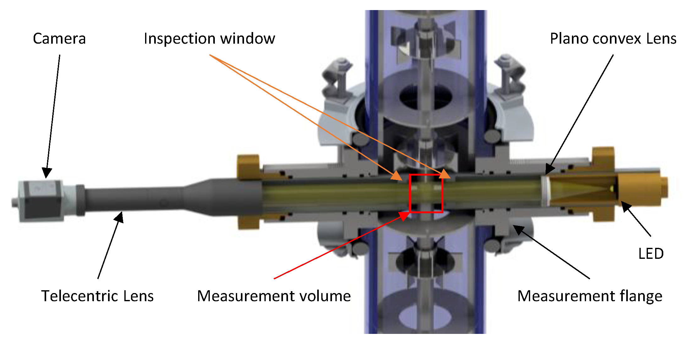
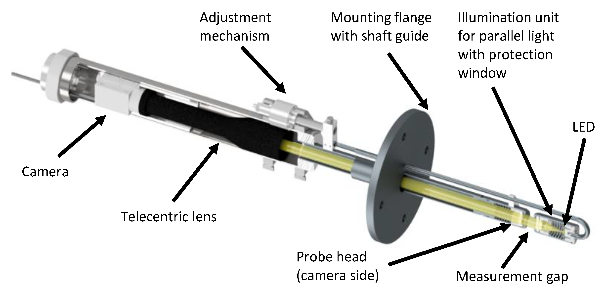
1.2. Optical Multimode Online Probe

The Optical Multimode Online Probe (OMOP) is an image-based shadowgraphic measurement technique, with an opposite based array [22] as depicted in Figure 1. One of the probe tubes contains an illumination unit that generates parallel light via a LED and a plan convex lens. The light passes out through an inspection window at the front end of the probe tube and afterwards through the measuring volume between the two diametrical probe tubes. On the opposite side, a camera with a telecentric lens acquires the resulting shadowgraphic image. The arrangement of illumination and lens result in images having high contrast and significantly better image quality compared to commercial incident light probes. In addition, at equal magnification, a significantly higher depth of field is achieved by telecentric lenses than by conventional entocentric lenses [23].

Telecentric optics use an aperture at the image-side focal point, whereby the image is formed exclusively by parallel light. This results in images with a distance-independent and constant magnification. In contrast, when images are taken with entocentric lenses, objects are projected at different sizes depending on their distance to the optics, which either requires calibration or leads otherwise to erroneous measurements. With telecentric systems, on the one hand, calibration is not necessary due to the constant magnification [24], and, on the other hand, the high contrast and greater depth of field make it much easier to evaluate images using simple image evaluation algorithms. With entocentric systems complex image processing algorithms are required even for simple evaluations at low holdup. The drawback of the first version of OMOP are a roughly four- to eightfold increase in installation space with the opposite illumination unit compared to incident light probes. Therefore, telecentric endoscope probes were developed to overcome the disadvantages [25], as a one-sided installation via a flange reduces the required installation space, but retains the complete measuring principle with adjustable size of the measurement gap and its position in the apparatus. In recent years, a probe for industrial-scale apparatuses has been developed that is inserted via a DN80 flange [26] and can be used for apparatus sizes from about DN450 to DN1000. In addition, the probe has been scaled down, and a laboratory probe [27] has been developed for a small apparatus between DN80 and DN600 and can be inserted via a DN40 [28] or DN50 [27] flange. In this work, the laboratory probe is used, which is depicted in Figure 2.

Although the method of probe insertion has been further developed, both a two-sided measuring flange and an endoscope probe can be usefully applied. Endoscopic probes are particularly useful for a large (<DN500) and existing apparatus, while two-sided measuring rings are mainly used at small scales (DN25-DN450), e.g., in pipes and small vessels.

In addition to these design improvements the application of the measurement technology has been extended to other multiphase flows and apparats, from extraction columns to mixer-settlers [29,30], reaction pumps [31], bubble columns [24,25,27,32], crystallization processes [28], evaporation [33] and spray regimes in distillation and absorption columns [34,35], where for the latter minor adaptions were necessary [36].

In order to determine the DSD from the experimental OMOP data, an image analysis using conventional image processing or neural networks (NN) is necessary. This includes binarization and, if necessary, watershed segmentation to segment touching or overlapping particles [32,37] as well as Hough transformation [38], which detects specific shaped objects in an image [38,39,40]. Unfortunately, conventional image processing algorithms are limited to images at low and medium phase fractions [41]. As to that, at higher phase fractions with strong overlapping, advanced image processing methods, like the use of NN [42] is an option.

However, it is necessary to train the NN in advance with extensive labeled data, which is rather time-consuming. Alternatively, a training with synthetic data using labeled training sets with known DSD is extremely effective. Schäfer et al. used computer generated synthetic data to train a Convolutional Neural Network (CNN) [43] at phase fractions up to 25 vol.-%. A detailed comparison between this technique and a commercially available probe for droplet detection can be found elsewhere [44].

1.3. Theory and Modelling

Based on the model of isotropic turbulence developed by Kolmogorov [45] the following expression (Equation (1)) was derived for the maximum stable droplet diameter in a fully turbulent flow at high Reynolds numbers:

$${\overline{u}}^2=C_1{\left(\overline{\epsilon }·d_{\max }\right)}^{2/3}$$

(1)

The mean relative velocity $\overline{u}$, caused by turbulent pressure fluctuations in the direction of the flow, is proportional to the mean energy dissipation $\overline{\epsilon }$ and the maximum stable droplet diameter d_max and a correlation coefficient C₁. Based on this theory, Hinze [46] derived a Weber number $W{e}_{\left(d\right)}$ for the maximum stable droplet diameter:

$$W{e}_{\left(d\right)}=\frac{E_{kin}}{E_{\sigma }}=\frac{{\rho }_c·{\overline{u}}^2·d}{{\sigma }_{d,c}}$$

(2)

Herein E_kin is the turbulent kinetic energy and E_σ is the surface energy, with the density of the continuous phase ${\rho }_d$, the mean relative velocity $\overline{u}$, the drop diameter d and the interfacial tension σ_d,c. If the turbulent kinetic energy and the surface energy are equal, the droplet is stable. According to Hinze a droplet remains stable at a Weber number $W{e}_{\left(d\right)}$ ≤ 1, otherwise it breaks up into one or more smaller droplets [46]. Substituting Equation (1) in Equation (2) gives:

$$W{e}_{\left(\mathrm{dmax},\mathrm{crit}\right)}=\frac{{\rho }_c{C}_2{\overline{\epsilon }}^{ 2/3}{d}_{\max }^{5/3}}{{\sigma }_{d,c}}$$

(3)

and rearranged for d_max is:

$$d_{\max }=C_2·W{e}_{\left(\mathrm{dmax},\mathrm{crit}\right)}^{-0.6}{\left(\frac{{\sigma }_{d,c}}{{\rho }_c}\right)}^{0.6}{\overline{\epsilon }}^{-0.4}=C_2{\left(\frac{{\sigma }_{d,c}}{{\rho }_c}\right)}^{0.6}{\overline{\epsilon }}^{-0.4}$$

(4)

with the correlation coefficient C₂. In stirred tanks, $\overline{\epsilon }$ is independent of the liquid properties according to the theory of isotropic turbulence:

$$\overline{\epsilon }=K{N}^3{D}^2$$

(5)

Herein N is the stirrer speed, D is the impeller diameter and K is a correlation coefficient that depends on the impeller design. With Equations (4) and (5) a basic model for droplet breakup in stirred vessels by Shinnar and Church [47] is as follows:

$$\frac{d_{\max }}{D}=C_3{\left(\frac{{\rho }_c{N}^2{D}^3}{{\sigma }_{d,c}}\right)}^{-0.6}=C_{3}W{e}_T^{-0.6}$$

(6)

This results in a proportionality of $d_{\max }\propto W{e}_T^{-0.6}$, whereby $W{e}_T$ is the Weber number of the tank and isotropic turbulence is assumed. Nowadays, stirred tank drop diameters are usually described by the Sauter mean diameter (see Section 2.4). In the work of Sprow [48], the mean diameters, e.g., d₅₀ or the Sauter mean diameter d₃₂ are linearly related to the maximum stable diameter via a correlation coefficient $C_4$ [49]:

$$d_{32}=C_4{d}_{\max }$$

(7)

This approach is much more practical for describing the droplet size, since the Sauter mean diameter is proportional to the specific surface area being essential for describing mass transfer processes.

The equations above only describe droplet breakage and are only valid at low holdup where coalescence is negligible. As technically relevant phase fractions are significantly higher, drop–drop interactions will occur, resulting in coalescence. As to that, Equation (6) is extended by a linear function considering the influence of the phase fraction [50]:

$$\frac{d_{32}}{D}=f_{\left(\phi \right)}{C}_{4}W{e}_T^{-0.6}=C_4\left(1+C_5\phi \right)W{e}_T^{-0.6}=C_4\left(1+C_5\phi \right)W{e}_T^{C_9}$$

(8)

In this commonly used approach, the correlation coefficient C₄ reflects the impeller design, while C₅ is for coalescence. The exponent for the Weber number in Equation (6) is valid in systems without coalescence, and some authors found C₉ as a function of the phase fraction φ [14,17]. Laso et al. [51] developed another interesting approach, which covers high disperse phase fractions with the general form as:

$$\frac{d_{32}}{D}=C_6{\phi }^{C_7}{\left(\frac{{\mu }_d}{{\mu }_c}\right)}^{C_8}W{e}_T^{c_9}=C_6{\phi }^{C_7}{\left(\frac{{\nu }_d{\rho }_d}{{\nu }_c{\rho }_c}\right)}^{C_8}W{e}_T^{c_9}$$

(9)

Herein μ is the dynamic and ν the kinematic viscosity with the index $c$ for the continuous phase and d for the disperse phase, with C₆ = 0.118, C₇ = 0.27, C₈ = −0.056 and C₉ = −0.4. Noteworthy is that it takes the phase fraction as a nonlinear function and the viscosities of both phases into account.

2. Materials and Methods

2.1. Substances

Demineralized water is used as continuous phase and paraffin oil (FC 2006, Fauth GmbH + Co. KG, Mannheim, Germany) as disperse phase. For standardization, demineralized water is adjusted by admixing 50 mmol/L Na₂SO₄. Thereby, the continuous phase is not altered in its physical properties as given in

Table 1. Physical properties of the used substances at a temperature of 20 °C.

Substance	Density ρ [kg/m3]	Kinematic Viscosity ν [mm2/s]	Interfacial Tension σd,c [mN/m]
Water + Na2SO4 (50 mmol/L)	1000	1.0	-
Paraffin oil FC 2006	825	13.1	53

. The standardization of the continuous water phase results in a defined electric conductivity of $8800$ µS/cm, which is necessary to guarantee measurement repeatability damping the influence of hardly detectable impurities on coalescence [48,52]. The density of the water/Na₂SO₄ solution and the oil are measured with a density meter (DMA55, Stabinger Messtechnik GmbH, Graz, Austria). The kinematic viscosity of the oil was measured with a viscometer (Viscoboy 2, LAUDA Scientific GmbH, Lauda-Königshofen, Germany), the value for water was taken from literature. The interfacial tension of oil in water was determined with a contact angle microscope (DataPhysics Instrument GmbH, Filderstadt, Germany) using the pendant drop method.

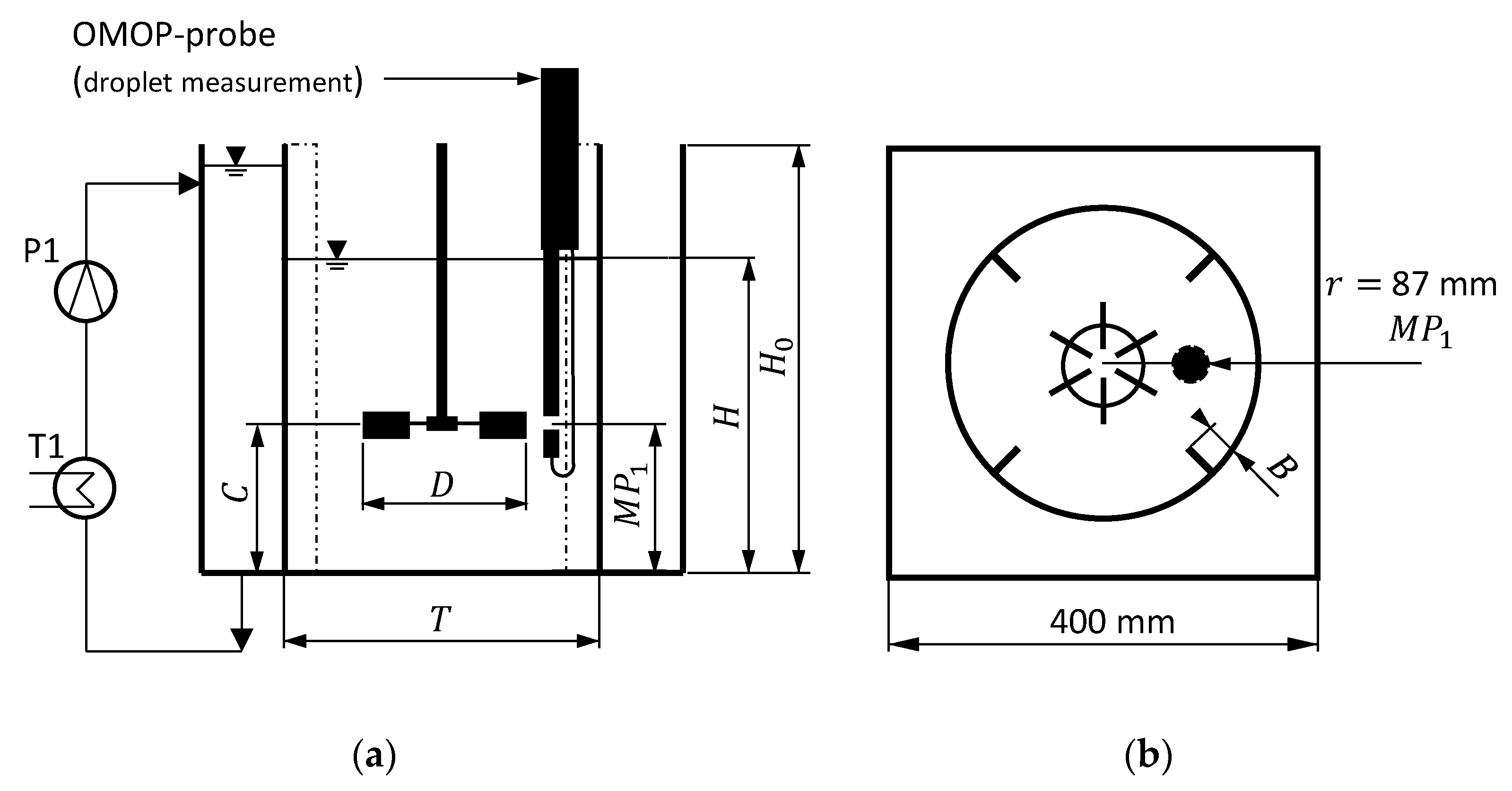
2.2. Experimental Setup

The experiments in this work are performed in a DN300 stirred tank shown in Figure 3. The tank is made of transparent polymethyl methacrylate (PMMA) and the geometry is based on a setup published by Montante et al. [53,54] with detailed measured velocity profiles [53,54]. Due to the same geometry, the data obtained in this study can be considered complementary to data from [54,55]. Therefore, an extensive database is available for CFD investigations, which have been presented on the same test case by, e.g., Rave et al. [55].

The tank has an inner diameter of T = 290 mm and a height of H₀ = 400 mm. The tank is filled to H = 290 mm height to ensure a ratio of H/T = 1. The tank is surrounded by another square tank, which is filled with water and ensures a constant temperature in the inner tank by means of thermostat T1 and pump P1. A six-blade Rushton impeller with a diameter of D = 98 mm (D/T ≈ 0.3) is positioned at an off-bottom-height C = T/2 = 145 mm and driven by a stirring unit (Heidolph RZR 2052 control). The impeller has the identical dimensions as in the work of Montante et al. [53,54], a disc diameter of 73.5 mm, a blade height of 19.6 mm, and a blade width of 24.5 mm. The tank is equipped with four radial equally distributed baffles. They have a width of B = T/10 = 29 mm, a thickness of 3 mm and cover the entire height H₀ of the tank.

The small single-sided probe (see Figure 2) is inserted vertically from above such that its measurement gap is located at the height of the impeller at measuring point MP₁. The measuring point is arranged radially at 87 mm from the center of the impeller shaft with an offset of 45° between two baffles. The probe is fitted with a Basler Aca 1300-60 gm camera and 1× telecentric lens. The chosen resolution is 1024 pixel × 1024 pixel, which equals 5.4 mm × 5.4 mm.

The camera with this lens results in a typical error range of +/−20 µm for measured lengths and diameters. The probe captures 1500 pictures at each measurement point with 10 fps. The gap between the probe heads, which form the measurement volume, was set to 2 mm. A further measuring point MP₂ near the liquid surface was additionally investigated experimentally up to 10 vol.-% and simulations are reported by Rave et al. [21].

2.3. Experimental Procedure

Experiments were performed at impeller speeds of N = 250, 325, 400 rpm. Phase fractions from φ = 5 vol.-% to 50 vol.-% are investigated in steps of 5 vol.-% at each impeller speed, whereby φ is defined according to Equation (10):

$$\phi =\frac{V_d}{V_d+V_c}$$

(10)

Here, V_d is the volume of the disperse phase and $V_c$ the volume of the continuous phase. Each experiment with a specific impeller speed N and phase fraction φ was carried out twice using the following routine.

At the beginning of each experiment, the tank was cleaned and the chemicals were weighed in the correct ratio. The thermostat and the pump for temperature control were switched on and the system was set to 20 °C. Na₂SO₄ was dissolved in the water and added to the tank and then the paraffin oil was added. The filling level $H$ was checked manually with a scale. Then, the impeller was turned on and a period of 40 min was used to ensure that a steady-state droplet size was established. The temperature of the emulsion was checked using a thermometer. After that, the droplet measurement is started taking 2.5 min to acquire the 1500 pictures. After each experiment, the chemicals were disposed and new ones were used for the next experiment in order to preclude a change in the physical properties due to long-term accumulation of impurities. Hence, for each impeller speed and phase fraction two droplet size measurements are available resulting from two separate experiments. One exception is the experiment for N = 400 rpm and φ = 5 vol.-%, which was measured only once without a repetition.

2.4. Data Analysis and Modelling

The images of the droplets captured by the camera are analyzed using a Convolutional Neural Network (CNN), which detects spherical droplets in a series of images to ensure statistical significance as depicted in Figure 4. The CNN is based on a U-net architecture using PyTorch with pre- and post-processing by the corresponding OpenCV functions. The CNN is specially trained for this use case as described elsewhere [43]. For the training of the CNN, the synthetic dataset from [43] was augmented with real images of droplets to increase the detection quality. In previous work, the detection of droplets with the CNN was validated up to φ = 25 vol.-% with an average error of 4.26% for the Sauter mean diameter. The CNN was used without any additional training for phase fractions φ ≥ 25 vol.-% and images were manually crosschecked to ensure accurateness.

The evaluated images show a precise detection of the droplets, whereas strongly overlapping droplets were not evaluated. Overall, more droplets were detected in the image at low phase fractions than at high phase fractions. In particular, Figure 4 shows that at 50 vol.-% only about half of the droplets were analyzed. However, since almost all detections are accurate, the network can be used for the evaluation of all phase fractions investigated. Overall, 15,000 to 300,000 droplets were detected per experiment, which is on average 100,000 droplets per experiment ensuring a statistic significance.

Crosschecking of the images revealed a few false detections for large droplets (diameters from 2 mm to 8 mm). Since these erroneous detections lead to false droplet sizes, they falsify the volume distribution and the Sauter mean diameter in particular. Therefore, 1% of droplets with the largest diameters were systematically excluded from the evaluation and not considered further.

The measured droplet diameters were converted to a number and volume distribution. The following relationship was used for the number distribution $q_{0,i}$:

$$q_{0,i}=\frac{\mathsf{\Delta }{Z}_i}{Z·\mathsf{\Delta }{d}_i} \mathrm{with} \mathsf{\Delta }{d}_i=d_i-d_{1-i}$$

(11)

The number distribution $q_{0,i}$ describes the number of particles, $\mathsf{\Delta }{Z}_i$, of all measured particles, Z, that are in a specific diameter range, $\mathsf{\Delta }{d}_i$, the so-called class width, which was set to 20 µm for all classes. The number distribution is suitable for showing phenomena such as unwanted emulsification, but has limited use for the description of mass transfer processes. The volume distribution, $q_{3,i}$, is calculated from the number distribution without considering any shape factor as follows:

$$q_{3,i}=\frac{{\overline{d}}_i^3·q_{0,i}}{{{\displaystyle \sum }}_{i=1}^n\left({\overline{d}}_i^3·q_{0,i}·\mathsf{\Delta }{d}_i\right)} \mathrm{with} {\overline{d}}_i=\frac{d_i+d_{i-1}}{2}$$

(12)

The volume distribution is more relevant for the description of mass transfer processes than the number distribution, since very small droplets contain almost no transfer component, and therefore have almost no contribution to mass transfer.

Although a complete DSD is decisive for a detailed description of processes, in many cases the Sauter mean diameter, d₃₂, is sufficient. It is calculated from the second moment, M_2,0 and third moment, M_3,0 of the number distribution as follows:

$$d_{32}=\frac{M_{3,0}}{M_{2,0}}=\frac{{{\displaystyle \sum }}_{i=1}^n\left(d_i^3·q_0·\mathsf{\Delta }{d}_i\right)}{{{\displaystyle \sum }}_{i=1}^n\left(d_i^2·q_0·\mathsf{\Delta }{d}_i\right)}$$

(13)

No shape factor was used, as the drops in the images are perfect circles (shape factor equals 1). Using the measured Sauter mean diameter and the given process parameters, the coefficients of Equations (8) and (9) are determined using the Thrust Region algorithm of the Matlab^® Curve Fitting Tool (Matlab^® version 9.6.0.1072779; R2019a and Curve Fitting Toolbox 3.5.9).

3. Results and Discussion

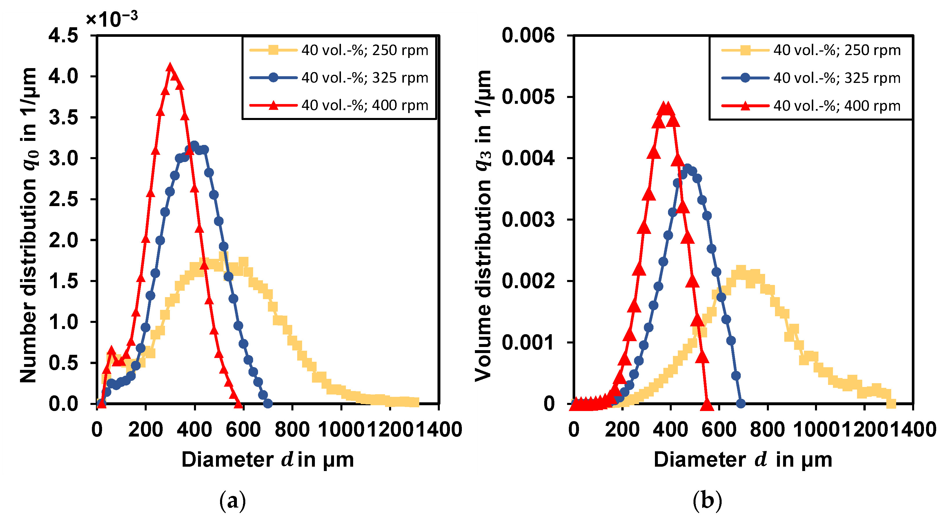
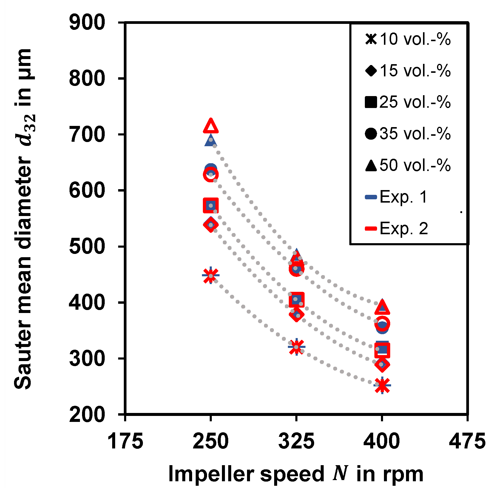
3.1. Influence of the Impeller Speed

The droplet diameters and the width of the distribution are mainly affected by the impeller speed [1,56]. Selected number distributions for the investigated impeller speed at φ = 40 vol.-% are exemplarily depicted in Figure 5a.

The shape of the measured number distributions in Figure 5a show a lognormal-distribution by trend. Local maxima in number distributions occur at the class $\overline{d}$ = 50 µm. These droplets are too small for further breakup or coalescence in this fine dispersion. Schäfer et al. [43] describe their CNN in combination with the presented camera and lens setup as poorly suited for small droplets, since the relative error for droplets smaller than d ≤ 80 µm exceeds 10%. This error is insignificant for the volume distribution q₃, since the fine dispersion has a negligible contribution to the volume distribution as depicted in Figure 5b. The volume distributions are nearly $q_{3,(<100 \mathsf{\mu }\mathrm{m})}$ ≈ 0 µm⁻¹ for particle classes smaller than 100 µm and are normally distributed in shape, which indicates a coalescing system [3]. As expected, the droplet size in the number as well as in the volume distribution decreases with increasing impeller speed. In addition, the distribution becomes narrower with increasing energy input and thus increasing impeller speed. This trend is observed for all experiments. DSD data of all q₀ and q₃ is given in the Supplementary material. For a simpler visualization of multiple experiments, Figure 6 depicts the Sauter mean diameters calculated according to Equation (13). The Sauter mean diameter decreases with increasing impeller speed. The qualitative trend of the Sauter mean diameter at different impeller speeds is similar for all phase fractions, with the trend shifting towards a larger droplet diameter for higher phase fractions.

All experimental data are in the typical error range. The average deviation of the Sauter mean diameter between two repetitions of an experiment (same impeller speed and phase fraction) is less than 4 µm and the maximum deviation, with one exception, is less than 9 µm, which confirms a high reproducibility. Small deviations are especially found for N = 250 rpm and are already discussed in the work of Rave et al. [24]. The largest error with approx. 25 µm is found at N = 250 rpm and φ = 50 vol.-% and could be caused by a slight malfunction of the CNN at those high phase fractions. All measured Sauter mean diameters and the number of measured particles are listed in the Supplementary Material in Tables S3–S48.

3.2. Influence of the Phase Fraction

As already seen in Figure 6, the DSD and the Sauter mean diameters are significantly affected by the phase fraction. The volume distributions in Figure 7a shifts towards larger droplets and becomes slightly broader with higher phase fractions. This effect is more pronounced for lower phase fractions than for higher ones. The experimental data for the phase fractions φ = 30 vol.-% and φ = 50 vol.-% in Figure 7a are almost identical. This indicates that the influence of the phase fraction on the DSD cannot be adequately represented by a linear function and that more complex functions have to be used. This effect was observed with all investigations within the typical error range of +/−20 µm. The Sauter mean diameter as a function of the phase fraction is depicted in Figure 7b. It decreases with increasing impeller speed. This is expected and reasonable since the mean energy dissipation increases with the impeller speed. An increase for the Sauter mean diameters is found for increasing phase fractions due to the higher collision rate of droplets.

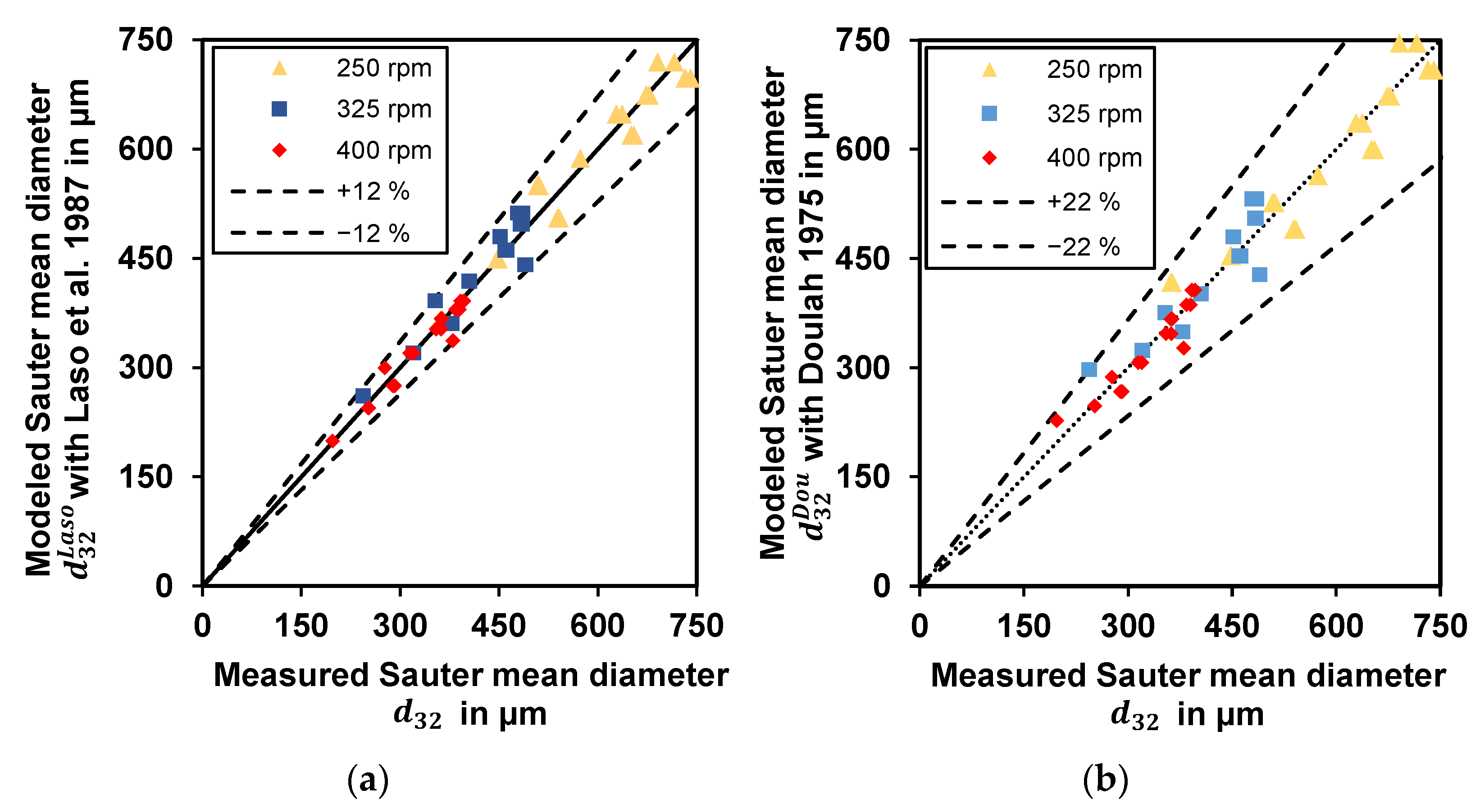
3.3. Modelling of the Sauter Mean Diameter

Table 2. Coefficients and confidence intervals for Equation (8) [50] and Equation (9) [51].

	Coefficients				Confidence Intervals
Values Equation (8)	C4	C5	C9	R2	C4	C5	C9
	0.1601	1.9190	−0.6456	0.9503	0.1113 to 0.2089	1.6180 to 2.2200	−0.6948 to −0.5964
Values Equation (9)	C6	C7	C9	R2	C6	C7	C9
	0.4283	0.2933	−0.6475	0.9719	0.3306 to 0.5260	0.2693 to 0.3173	−0.6845 to −0.6105

lists the coefficients and their corresponding confidence intervals of Equations (8) and (9), which were determined in this work.

Table 3. Absolute and relative deviations of the models.

	Calculated Errors
	Maximum Relative Error	Mean Relative Error	Maximum Absolute Error	Mean Absolute Error
	$$\begin{gathered} \mathsf{\Delta }{\mathit{d}}_{32}^{\mathit{m}\mathit{a}\mathit{x},\mathit{\%}} \\ \mathbf{in} \% \end{gathered}$$	$$\begin{gathered} \mathsf{\Delta }{\overline{\mathit{d}}}_{32}^{\mathit{m}\mathit{e}\mathit{a}\mathit{n},\mathit{\%}} \\ \mathbf{in} \% \end{gathered}$$	$$\begin{gathered} \mathsf{\Delta }{\mathit{d}}_{32}^{\mathit{m}\mathit{a}\mathit{x},\mathsf{\mu }\mathbf{m}} \\ \mathbf{in} \mu \mathbf{m} \end{gathered}$$	$$\begin{gathered} \mathsf{\Delta }{\overline{\mathit{d}}}_{32}^{\mathit{m}\mathit{e}\mathit{a}\mathit{n},\mathsf{\mu }\mathbf{m}} \\ \mathbf{in} \mu \mathbf{m} \end{gathered}$$
Values Equation (8)	21.9	5.7	63	24
Values Equation (9)	11.4	4.0	50	18

summarizes the quality of the re-correlated models. The coefficient C₈ of the viscosity in Equation (9) was taken from the data of Laso et al. [51], because the influence of the viscosity is not studied in this work.

Both models show a good agreement with the measured values (see Figure 8), which is confirmed by high coefficients of determination, R² > 0.95. The model of Laso et al. [51] represents the experimental data slightly better (higher value of R²). The deviation from the model to the experimental data is less than 12% absolute and 4.0% as mean deviation for Laso et al. [51] and less than 22% absolute and 5.7% as mean deviation for Doulah [50]. The errors are randomly distributed with the approach of Laso et al. [51], over all data. The standard approach by Doulah [50] has the highest errors for φ = 5 vol.-%, which is a result of the linear dependence of the phase fraction in the model. The value of the Weber exponent is for both models around C₉ ≈ −0.65, which is close to the theoretical one of −0.6 being obtained if coalescence is neglected [47]. The results with a Weber exponent C₉ = −0.6 are shown in the Supplementary Material in Tables S1 and S2 and in Figure S1.

4. Conclusions

In this work, a telecentric endoscopic transmitted light probe was used to measure the droplet size in a DN300 stirred vessel near the impeller region. The DSD was measured at phase fractions between φ = 5 vol.-% to 50 vol.-% and impeller speeds between N = 250 rpm and 400 rpm. The endoscopic probe can be easily installed and the measurement technique including a CNN based analysis is appropriate for the characterization of liquid-liquid systems with industrially relevant phase fractions up to φ = 50 vol.-%. In addition, large quantities of droplets can be reliably detected resulting in statistically significant and highly resolved DSD with at least 10,000 droplets per distribution. A repetition of the experiments showed minimal deviations for the same experimental parameters within the typical error range of approx. 20 µm. It could be shown, that telecentric shadowgraphic probes with a modern image analysis based on a CNN can be utilized to accurately characterize particulate liquid–liquid flows at industrial relevant phase fractions.

The experimental results show, that the impeller speed as well as the phase fraction mainly affect the Sauter mean diameter in stirred vessels. Especially the latter has a strong influence below a phase fraction of φ ≤ 30 vol.-%. For higher phase fractions, the influence is marginal and can be neglected. Two models from literature were re-correlated [50,51] and adequately represent the experimental data within relative deviations of 12% [51] and 22% [50]. As expected, the experimental data is better represented by the approach of Laso et al. [51] than by the standard approach [50], which can be explained by the additional substance properties that were taken into account.

The enhancement and validation of image analysis techniques in combination with telecentric shadowgraphic probes are part of future work, especially with a focus on industrial phase fractions and apparatus geometries. This new technique discussed here enables the improvement and development of models for the prediction of the behavior of dispersions and other particulate multiphase flows. Possible future applications are manifold, like the detection of cavitation bubbles, the measurement of bubbles in jet-loop-reactors or the use in fixed bed reactors for the characterization of the flow regime to name a few.

References

1. Kraume, M. Transportvorgänge in der Verfahrenstechnik; Springer: Berlin/Heidelberg, Germany, 2012. [Google Scholar]
2. Kresta, S.M.; Etchells, A.W.; Dickey, D.S.; Atiemo-Obeng, V.A. (Eds.) Advances in Industrial Mixing: A Companion to the Handbook of Industrial Mixing; Wiley: Hoboken, NJ, USA, 2016. [Google Scholar]
3. Zerfa, M.; Brooks, B.W. Prediction of vinyl chloride drop sizes in stabilised liquid-liquid agitated dispersion. Chem. Eng. Sci. 1996, 51, 3223–3233. [Google Scholar] [CrossRef]
4. Cull, S.G.; Lovick, J.W.; Lye, G.J.; Angeli, P. Scale-down studies on the hydrodynamics of two-liquid phase biocatalytic reactors. Bioprocess Biosyst. Eng. 2002, 25, 143–153. [Google Scholar] [PubMed]
5. Angle, C.W.; Hamza, H.A. Predicting the sizes of toluene-diluted heavy oil emulsions in turbulent flow Part 2: Hinze–Kolmogorov based model adapted for increased oil fractions and energy dissipation in a stirred tank. Chem. Eng. Sci. 2006, 61, 7325–7335. [Google Scholar] [CrossRef]
6. Abidin, M.I.I.Z.; Raman, A.A.A.; Nor, M.I.M. Review on Measurement Techniques for Drop Size Distribution in a Stirred Vessel. Ind. Eng. Chem. Res. 2013, 52, 16085–16094. [Google Scholar] [CrossRef]
7. Kumar, S.; Ganvir, V.; Satyanand, C.; Kumar, R.; Gandhi, K.S. Alternative mechanisms of drop breakup in stirred vessels. Chem. Eng. Sci. 1998, 53, 3269–3280. [Google Scholar] [CrossRef]
8. EL-Hamouz, A.; Cooke, M.; Kowalski, A.; Sharratt, P. Dispersion of silicone oil in water surfactant solution: Effect of impeller speed, oil viscosity and addition point on drop size distribution. Chem. Eng. Processing 2009, 48, 633–642. [Google Scholar] [CrossRef]
9. Maaß, S.; Wollny, S.; Voigt, A.; Kraume, M. Experimental comparison of measurement techniques for drop size distributions in liquid/liquid dispersions. Exp. Fluids 2011, 50, 259–269. [Google Scholar] [CrossRef]
10. Lovick, J.; Mouza, A.A.; Paras, S.V.; Lye, G.J.; Angeli, P. Drop size distribution in highly concentrated liquid-liquid dispersions using a light back scattering method. J. Chem. Technol. Biotechnol. 2005, 80, 545–552. [Google Scholar] [CrossRef]
11. Barrett, P.; Glennon, B. In-line FBRM Monitoring of Particle Size in Dilute Agitated Suspensions. Part. Part. Syst. Charact. 1999, 16, 207–211. [Google Scholar] [CrossRef]
12. Barrett, P.; Glennon, B. Characterizing the Metastable Zone Width and Solubility Curve Using Lasentec FBRM and PVM. Chem. Eng. Res. Des. 2002, 80, 799–805. [Google Scholar] [CrossRef] [Green Version]
13. Lichti, M.; Bart, H.-J. Particle Measurement Techniques in Fluid Process Engineering. Chembioeng. Rev. 2018, 5, 79–89. [Google Scholar] [CrossRef]
14. Amokrane, A.; Maaß, S.; Lamadie, F.; Puel, F.; Charton, S. On droplets size distribution in a pulsed column. Part I: In-situ measurements and corresponding CFD–PBE simulations. Int. J. Chem. Eng. 2016, 296, 366–376. [Google Scholar] [CrossRef]
15. Schlüter, M. Lokale Messverfahren für Mehrphasenströmungen. Chem. Ing. Tech. 2011, 83, 992–1004. [Google Scholar] [CrossRef]
16. Godfrey, J.C.; Grilc, V. (Eds.) Drop Size and Drop Size Distributions for Liquid-Liquid Dispersions in Agitated Tanks of Square Cross Section. In Proceedings of the 2nd European Conference on Mixing, Cambridge, UK, 22–27 June 1977; BHRA Fluid Engineering: Cambridge, UK, 1977; pp. 1–20. [Google Scholar]
17. Desnoyer, C.; Masbernat, O.; Gourdon, C. Experimental study of drop size distributions at high phase ratio in liquid–liquid dispersions. Chem. Eng. Sci. 2003, 58, 1353–1363. [Google Scholar] [CrossRef]
18. Qi, L.; Meng, X.; Zhang, R.; Liu, H.; Xu, C.; Liu, Z.; Klusener, P.A.A. Droplet size distribution and droplet size correlation of chloroaluminate ionic liquid–heptane dispersion in a stirred vessel. Int. J. Chem. Eng. 2015, 268, 116–124. [Google Scholar] [CrossRef]
19. Kraume, M.; Gäbler, A.; Schulze, K. Influence of Physical Properties on Drop Size Distribution of Stirred Liquid-Liquid Dispersions. Chem. Eng. Technol. 2004, 27, 330–334. [Google Scholar] [CrossRef]
20. Gäbler, A.; Wegener, M.; Paschedag, A.R.; Kraume, M. The effect of pH on experimental and simulation results of transient drop size distributions in stirred liquid–liquid dispersions. Chem. Eng. Sci. 2006, 61, 3018–3024. [Google Scholar] [CrossRef]
21. Rave, K.; Hermes, M.; Wirz, D.; Hundshagen, M.; Friebel, A.; Harbou, E.V.; Bart, H.-J.; Skoda, R. Experiments and fully transient coupled CFD-PBM 3D flow simulations of disperse liquid-liquid flow in a baffled stirred tank. Chem. Eng. Sci. 2022, 120, 117518. [Google Scholar] [CrossRef]
22. Mickler, M.; Bart, H.-J. Optical Multimode Online Probe: Erfassung und Analyse von Partikelkollektiven. Chem. Ing. Tech. 2013, 85, 901–906. [Google Scholar] [CrossRef]
23. Schuhmann, R.; Thöniß, T. Telezentrische Systeme fuer die optische Mess- und Prueftechnik. Technol. Mess 1998, 65, 131–136. [Google Scholar] [CrossRef]
24. Wirz, D.; Bart, H.-J. Advances in particle size analysis with transmitted light techniques. Bulg. Chem. Commun. 2020, 52, 554–560. [Google Scholar]
25. Lichti, M. Optische Erfassung von Partikelmerkmalen: Entwicklung einer Durchlichtmesstechnik für Apparate der Fluidverfahrenstechnik. Ph. D. Thesis, TU Kaiserslautern, Kaiserslautern, Germany, 2018. [Google Scholar]
26. Lichti, M.; Roth, C.; Bart, H.-J. Vorrichtung für Bildaufnahmen eines Messvolumens in Einem Behälter. Patent DE102015103497A1, 15 September 2016. [Google Scholar]
27. Lichti, M.; Cheng, X.; Stephani, H.; Bart, H.-J. Online Detection of Ellipsoidal Bubbles by an Innovative Optical Approach. Chem. Eng. Technol. 2019, 42, 506–511. [Google Scholar] [CrossRef]
28. Wirz, D.; Hofmann, M.; Lorenz, H.; Bart, H.-J.; Seidel-Morgenstern, A.; Temmel, E. A Novel Shadowgraphic Inline Measurement Technique for Image-Based Crystal Size Distribution Analysis. Crystals 2020, 10, 740. [Google Scholar] [CrossRef]
29. Steinhoff, J.; Bart, H.-J. Settling Behavior and CFD Simulation of a Gravity Separator. In Extraction 2018; The Minerals, Metals & Material Series; Davis, B.R., Moats, M.S., Wang, S., Gregurek, D., Kapusta, J., Battle, T.P., Schlesinger, M.E., Flores, G.R.A., Jak, E., Goodall, G., et al., Eds.; Springer International Publishing: Cham, Switzerland, 2018; pp. 1997–2007. [Google Scholar]
30. Steinhoff, J.; Charlafti, E.; Reinecke, L.; Kraume, M.; Bart, H.-J. Investigation and development of gravity separators with a standardized experimental setup. Can. J. Chem. Eng. 2020, 98, 384–393. [Google Scholar] [CrossRef]
31. Schmitt, P.; Hlawitschka, M.W.; Bart, H.-J. Centrifugal pumps as extractors. Chem. Ing. Tech. 2020, 262, 12215. [Google Scholar] [CrossRef] [Green Version]
32. Lichti, M.; Bart, H.-J. Bubble size distributions with a shadowgraphic optical probe. Flow Meas. Instrum. 2018, 60, 164–170. [Google Scholar] [CrossRef]
33. Jasch, K.; Schulz, J.; Bart, H.-J.; Scholl, S. Droplet Entrainment Analysis in a Flash Evaporator with an Image-Based Measurement Technique. Chem. Ing. Tech. 2021, 93, 1071–1079. [Google Scholar] [CrossRef]
34. Schulz, J.; Usslar, M.; Bart, H.-J. Impact of weir design on entrained liquid in tray columns. AIChE J. 2021, 67, A483. [Google Scholar] [CrossRef]
35. Schulz, J.; Bart, H.-J. Analysis of entrained liquid by use of optical measurement technology. Chem. Eng. Res. Des. 2019, 147, 624–633. [Google Scholar] [CrossRef]
36. Schulz, J. Local Image-Based and Conventional Integral Entrainment Analysis; Shaker Verlag: Düren, Germany, 2021. [Google Scholar]
37. Lichti, M.; Schulz, J.; Bart, H.-J. Quantification of Entrainment Using an Optical Inline Probe. Chem. Ing. Tech. 2019, 91, 429–434. [Google Scholar] [CrossRef]
38. Hough, P.V.C. Method and Means for Recognizing Complex Patterns. U.S. Patent US3069654A, 18 December 1962. [Google Scholar]
39. Yuen, H.K.; Princen, J.; Illingworth, J.; Kittler, J. Comparative study of Hough Transform methods for circle finding. Image Vis. Comput. 1990, 8, 71–77. [Google Scholar] [CrossRef] [Green Version]
40. Illingworth, J.; Kittler, J. A survey of the hough transform. Comput. Graph. Image Processing 1988, 44, 87–116. [Google Scholar] [CrossRef]
41. Mickler, M.; Didas, S.; Jaradat, M.; Attarakih, M.; Bart, H.-J. Tropfenschwarmanalytik mittels Bildverarbeitung zur Simulation von Extraktionskolonnen mit Populationsbilanzen. Chem. Ing. Tech. 2011, 83, 227–236. [Google Scholar] [CrossRef]
42. LeCun, Y.; Bengio, Y.; Hinton, G. Deep learning. Nature 2015, 521, 436–444. [Google Scholar] [CrossRef] [PubMed]
43. Schäfer, J.; Schmitt, P.; Hlawitschka, M.W.; Bart, H.-J. Measuring Particle Size Distributions in Multiphase Flows Using a Convolutional Neural Network. Chem. Ing. Tech. 2019, 83, 992. [Google Scholar] [CrossRef] [Green Version]
44. Steinhoff, J.; Charlafti, E.; Leleu, D.; Reinecke, L.; Becker, K.; Kalem, M.; Sixt, M.; Franken, H.; Braß, M.; Borchardt, D.; et al. ERICAA, Energie- und Ressourceneinsparung durch Innovative und CFD-Basierte Auslegung von Flüssig/Flüssig-Schwerkraftabscheidern, Abschlussbericht; Wiley: Hoboken, NJ, USA, 2019. [Google Scholar]
45. Kolmogorov, A. The Local Structure of Turbulence in Incompressible Viscous Fluid for Very Large Reynolds’ Numbers. Dokl. Akad. Nauk SSSR 1941, 30, 301–305. [Google Scholar]
46. Hinze, J.O. Fundamentals of the hydrodynamic mechanism of splitting in dispersion processes. AIChE J. 1955, 1, 289–295. [Google Scholar] [CrossRef]
47. Shinnar, R.; Church, J.M. Statistical theories of turbulence in predicting particle size in agitated dispersions. Ind. Eng. Chem. 1960, 52, 253–256. [Google Scholar] [CrossRef]
48. Gebauer, F. Fundamentals of Binary Droplet Coalescence in Liquid–Liquid Systems; Verlag Dr. Hut GmbH: München, Germany, 2018. [Google Scholar]
49. Sprow, F.B. Distribution of drop sizes produced in turbulent liquid—liquid dispersion. Chem. Eng. Sci. 1967, 22, 435–442. [Google Scholar] [CrossRef]
50. Doulah, M.S. An effect of hold-up on drop sizes in liquid-liquid dispersions. Ind. Eng. Chem. 1975, 14, 137–138. [Google Scholar] [CrossRef]
51. Laso, M.; Steiner, L.; Hartland, S. Dynamic simulation of agitated liquid—liquid dispersions—II. Experimental determination of breakage and coalescence rates in a stirred tank. Chem. Eng. Sci. 1987, 42, 2437–2445. [Google Scholar] [CrossRef]
52. Villwock, J.; Gebauer, F.; Kamp, J.; Bart, H.-J.; Kraume, M. Systematic Analysis of Single Droplet Coalescence. Chem. Eng. Technol. 2014, 37, 1103–1111. [Google Scholar] [CrossRef]
53. Montante, G.; Lee, K.C.; Brucato, A.; Yianneskis, M. Numerical simulations of the dependency of flow pattern on impeller clearance in stirred vessels. Chem. Eng. Sci. 2001, 56, 3751–3770. [Google Scholar] [CrossRef]
54. Montante, G.; Brucato, A.; Lee, K.C.; Yianneskis, M. An experimental study of double-to-single-loop transition in stirred vessels. Can. J. Chem. Eng. 1999, 77, 649–659. [Google Scholar] [CrossRef]
55. Rave, K.; Lehmenkühler, M.; Wirz, D.; Bart, H.-J.; Skoda, R. 3D flow simulation of a baffled stirred tank for an assessment of geometry simplifications and a scale-adaptive turbulence model. Chem. Eng. Sci. 2021, 231, 116262. [Google Scholar] [CrossRef]
56. Zlokarnik, M. Stirring: Theory and Practice; Wiley-VCH: Weinheim, Germany; Chichester, UK, 2010. [Google Scholar]
Figure 1. Scheme of a OMOP in a DN100 extraction column. The invasive tubes are mounted eccentric and do not interfere with the impeller shaft.
Applsci 12 04069 g001
Figure 2. Endoscopic probe at laboratory scale. The mounting flange is adaptable to DN40 or larger.
Applsci 12 04069 g002
Figure 3. Experimental setup of the DN300 stirred vessel and the measurement position MP1 of the OMOP probe; (a) side view and (b) top view of the vessel.
Applsci 12 04069 g003
Figure 4. CNN analysis at different phase fractions at N = 325 rpm. (a) 10 vol.-%, (b) 30 vol.-% and (c) 50 vol.-%. The green circles represent the detected droplet circumference.
Applsci 12 04069 g004
Figure 5. (a) Number distribution at different rpm at φ = 40 vol.-% phase fraction; (b) volume distribution at different rpm at φ = 40 vol.-% phase fraction. The lines are a guide to the eye.
Applsci 12 04069 g005
Figure 6. Experimental Sauter mean diameter (experiment 1: blue solid symbols, repetition experiment 2: red hollow symbols) at different rpm and phase fractions (dotted lines are a guide to the eye).
Applsci 12 04069 g006
Figure 7. (a) Experimental volume distributions at different phase fractions, N = 400 rpm. The lines are a guide to the eye; and (b) experimental Sauter mean diameters of both experiments at different rpm (model of Laso et al. [51] with the coefficients from Table 2).
Applsci 12 04069 g007
Figure 8. Parity plot: (a) model of Laso et al. [51] within 12% error, (b) model of Doulah [50] within 22% error (coefficients from Table 2).
Applsci 12 04069 g008