Tool for Predicting College Student Career Decisions: An Enhanced Support Vector Machine Framework

Abstract

The goal of this research is to offer an effective intelligent model for forecasting college students’ career decisions in order to give a useful reference for career decisions and policy formation by relevant departments. The suggested prediction model is mainly based on a support vector machine (SVM) that has been modified using an enhanced butterfly optimization approach with a communication mechanism and Gaussian bare-bones mechanism (CBBOA). To get a better set of parameters and feature subsets, first, we added a communication mechanism to BOA to improve its global search capability and balance exploration and exploitation trends. Then, Gaussian bare-bones was added to increase the population diversity of BOA and its ability to jump out of the local optimum. The optimal SVM model (CBBOA-SVM) was then developed to predict the career decisions of college students based on the obtained parameters and feature subsets that are already optimized by CBBOA. In order to verify the effectiveness of CBBOA, we compared it with some advanced algorithms on all benchmark functions of CEC2014. Simulation results demonstrated that the performance of CBBOA is indeed more comprehensive. Meanwhile, comparisons between CBBOA-SVM and other machine learning approaches for career decision prediction were carried out, and the findings demonstrate that the provided CBBOA-SVM has better classification and more stable performance. As a result, it is plausible to conclude that the CBBOA-SVM is capable of being an effective tool for predicting college student career decisions.

1. Introduction

With the advancement of technology and the development of society, the world today has become more challenging and uncertain. It can be said that we are now in the VUCA era, which is characterized by volatility, uncertainty, complexity, and ambiguity. The frequent “black swan events” in recent years and the new crown epidemic that swept the world this year are two very prominent examples [1]. In such an uncertain VUCA era, it is crucial for everyone to find their own positioning and future development direction. As a special group, college students are the backbone of China’s future society and the group of people who are responsible for China’s dream of achieving great rejuvenation. Thus, having strong career development ability is a requirement for their comprehensive quality and professionalism and also reflects their learning achievements in their college career. In September 2019, the Ministry of Education issued “the Opinions on Deepening the Reform of Undergraduate Education and Teaching to Comprehensively Improve the Quality of Talent Training”, proposing to “deepen the reform of the education and teaching system”, “develop personalized training programs and academic career plans” for college students, and “build a professional setting management system oriented to economic and social development and students’ career development needs”. The career development of college students is closely related to their academic career and career, and it is also related to the results of undergraduate education and teaching reform and the quality of talent cultivation, which are valued at the national level.

In recent years, especially since the Ministry of Education issued the notice of “Teaching Requirements of Career Development and Career Guidance Course for College Students”, career planning education has been in full swing in all colleges and universities, and the career development of college students has received attention from the state, society, colleges and universities, and scientific research institutions at all levels. There are many pieces of research on the career development of college students, but the existing research mainly focus on career education and guidance and career theory and application, while there is a lack of further exploration on the empirical research and model construction of college students’ career development; there is especially still a lot of room for exploration in combining the latest theoretical research results with the characteristics of Chinese local students at present. Since 2018, with the entry of “post-00” college students into colleges and universities, “post-00” college students have accounted for half of the population so far. The “post-00s” college students have a strong sense of autonomy, which is reflected in their desire to choose their own learning style, major direction, and life circle according to their own interests. They have a strong sense of self-awareness and self-identity, which is reflected in their courage to express and insist on their own opinions; they have pragmatic and rational life goals and realization paths, which is reflected in their belief that success mainly depends on personal efforts. After sorting out these characteristics, it is found that the Self-Determination Theory (SDT), which is currently the focus of academic circles, is in line with the characteristics of college students as the research target and the characteristics of the times.

According to Deci Edward L. and Professor Ryan Richard M., two well-known American psychologists, self-determination theory was first suggested in the 1980s and is a cognitive-motivational explanation of human self-determined action [2]. Those who believe in self-determination theory believe that people are active creatures who possess an inbuilt capacity for self-determination and psychological growth. This potential leads people to engage in interest-oriented behaviors that are conducive to the development of their abilities, and this innate motivation for self-determination constitutes an intrinsic motivation for human behavior. After several decades of research and development, self-determination theory has gradually formed a relatively complete theoretical system on human motivation and personality, which has been widely applied in the fields of organizational management, sports, psychological medicine, and educational counseling [3].

“Autonomy needs” are about having the psychological freedom to do things of one’s own choice, “Competence needs” are about having control over one’s environment and growing as a person, and “Belonging needs”, also called relationship needs, are about having a sense of connection with other people. These three needs are important for people to grow, internalize, and be happy [4]. The main assumption of this theory is that when the three basic psychological needs of autonomy, competence, and relationship are met, people will be more willing and able to participate in activities, which will lead to more sustained and high-quality behaviors and better behavioral outcomes as well as better physical and mental health for people. At the same time, we find that the three basic psychological needs are very individualized and, interestingly, can exist widely across cultures and situations. Through a literature review, the core assumptions of self-determination theory are consistent with the characteristics of college students; therefore, it is feasible to discuss the construction of a career development model for college students based on self-determination theory.

Until now, many studies have been conducted to better investigate and discuss the career development of college students. Using interview data from product development interns at a single engineering business, Powers et al. [5] contributed insights into the particular abilities that interns describe as gaining in their internship and identified linkages between school-and-work learning. Kim et al. [6] used a sample of 420 South Korean college students to analyze the cultural validity of the family impact scale in order to determine the degree to which family played a role in college students’ career development within collectivistic societies. Kiselev et al. [7] addressed the social constructivism foundations of machine learning approaches in career advising, as well as the relevance of social networks in psychological research. Chung et al. [8] employed random forests in machine learning to predict students at risk of dropping out in order to identify and assist students who are in danger of dropping out. Luo et al. [9] looked at how stereotyped attitudes about STEM occupations influenced STEM self-efficacy and STEM career-related result expectancies as well as how these constructs predicted STEM career desire in upper primary pupils. Nauta et al. [10] looked at the effects of interpersonal interactions on gay, lesbian, bisexual, and heterosexual college students’ job decisions. Park et al. [11] investigated the impacts of a future time perspective on job selections, which comprised three sessions that were opportunity, value, and connectivity. By collecting 558 completed questionnaires, Lee et al. [12] investigated the influence of several significant professional decision-making elements (i.e., advisers, industry mentors, parents, faculty members, and social media) on students.

Therefore, in order to discuss the construction of a career development model for college students based on self-determination theory, this paper proposes a support vector machine (SVM) combined with improved butterfly optimization algorithm (BOA) named CBBOA that adds two mechanisms to BOA. First, a communication mechanism (CM) was added, which can enhance the exploitation ability and improve the convergence accuracy of the original BOA. We also introduced Gaussian bare-bones mechanism into the original BOA. Mutation mechanism in Gaussian bare-bones can increase the diversity of the population and avoid falling into local optimum. In addition, in view of the shortcomings of SVM, we propose a new CBBOA-SVM model, which can substantially improve the classification accuracy of the original SVM by optimizing the parameters. In order to verify the effectiveness of the proposed CBBOA, we conducted a series of experiments based on benchmark functions. Simulation results illustrate that the algorithm showed better performance than the original BOA. In order to better study the career decision factors of college students, it is necessary to conduct comparative experiments between CBBOA-SVM and other algorithms. The results show that CBBOA-SVM can produce more accurate classification results as well as greater stability in terms of the four indicators studied when compared to all other comparison methods.

The following are some of its most significant contributions:

• An enhanced BOA (CBBOA) is proposed, where a communication mechanism is used to boost the exploitation ability of the convergence accuracy, as well as a Gaussian bare-bones mechanism is utilized to raise the diversity of the population and the capacity of avoiding falling into local optimum.
• A new CBBOA-SVM with a feature selection model is developed to predict the future career decisions of college students, which can aid jobless college students in selecting acceptable occupations for themselves but also help the government’s macro-management of college students’ employment market.
• The performance of CBBOA is experimentally verified by comparing the high-quality algorithm with CBBOA, which shows that the performance of CBBOA is better than other peers.
• To further validate the performance of CBBOA-SVM with feature selection, we compared it with five other similar methods, which indicates that it has a better performance than other similar methods and can be used to study the impact of career decisions.

The remainder of the paper’s structure is depicted below. The proposed CBBOA model and the CBBOA-SVM model are described in detail in Section 2 and Section 3, respectively. Section 4 is primarily concerned with the introduction of the data source and simulation settings. On the real-world dataset, the experimental results of CBBOA on benchmark functions and CBBOA-SVM on the benchmark functions are discussed in Section 5. Section 6 is devoted primarily to the discussion of the improved algorithm and its implications. Finally, there is a section dedicated to summaries and advice.

2. Proposed CBBOA

CBBOA has added two mechanisms compared with the original BOA. These two mechanisms are the communication mechanism and Gaussian Bare-Bones, respectively. The two mechanisms and the main flow of the proposed CBBOA are described in detail in the remainder of this section.

2.1. Communication Mechanism (CM)

This communication mechanism (CM) is inspired by DE [13] and proposed in the recent work [13]. CM will select one individual in the population to communicate with other two optimal individuals in the population, thus generating the location of new individuals. This updated approach will enhance the exploitation capabilities. The updated formula of CM is as follows:

$$X_i^{t+1}=a\cdot X_i^t+\left(1-a\right)\cdot \left(S\left(1\right)+S\left(2\right)\right)/2$$

(1)

where a is a random number in the range [0, 1]; $X_i^t$ represents the i-th individual in the population in the t-th iteration; $S\left(1\right)$ and $S\left(2\right)$ represent the two best individuals in the population.

2.2. Gaussian Bare-Bones

Gaussian Bare-Bones has been widely used in other algorithms. For example, Kennedy et al. [14] proposed bare-bones particle swarms optimization (BBPSO), and Omran et al. [15] proposed bare-bones differential evolution (BBDE) through this mechanism. Of course, the application of Gaussian Bare-Bones in these algorithms has changed and improved. In this paper, one of the updated formulas of Gaussian Bare-Bones adopts a new Gaussian variation strategy proposed by Wang et al. [16]. The formula of the Gaussian variation strategy is as follows:

$$x_{i,j}^{t+1}=N\left(mu, sigma\right)$$

(2)

where $N\left(mu,sigma\right)$ means a random generation from a Gaussian distribution with the mean of $mu=\left(x_{best,j}+x_{i,j}\right)/2$ and the standard deviation of $sigma=\left|x_{best,j}-x_{i,j}\right|$.

In this paper, in addition to the Gaussian variation mentioned above, another formula adopts the variation mutation strategy based on DE. The two mutation methods can effectively increase the population diversity and prevent the algorithm from falling into local optimum. The complete Gaussian Bare-Bones update formula is as follows:

$$x_{i,j}^{t+1}=\{\begin{array}{c}N\left(mu, sigma\right) rand<CR \left(1\right)\\ x_{i_1,j}^t+k*\left(x_{i_2,j}^t-x_{i_3,j}^t\right) rand\ge CR \left(2\right)\end{array}$$

(3)

where CR is the predetermined mutation probability. $x_{i_1,j}^t$, $x_{i_2,j}^t$ and $x_{i_3,j}^t$ are the $i_1$th population, the $i_2$th and the $i_3$th individual components in the jth dimension respectively. $i_1$, $i_2$ and $i_3$ are three random numbers between [1, N], and $i_1\ne i_2\ne i_3$.

2.3. Description of CBBOA

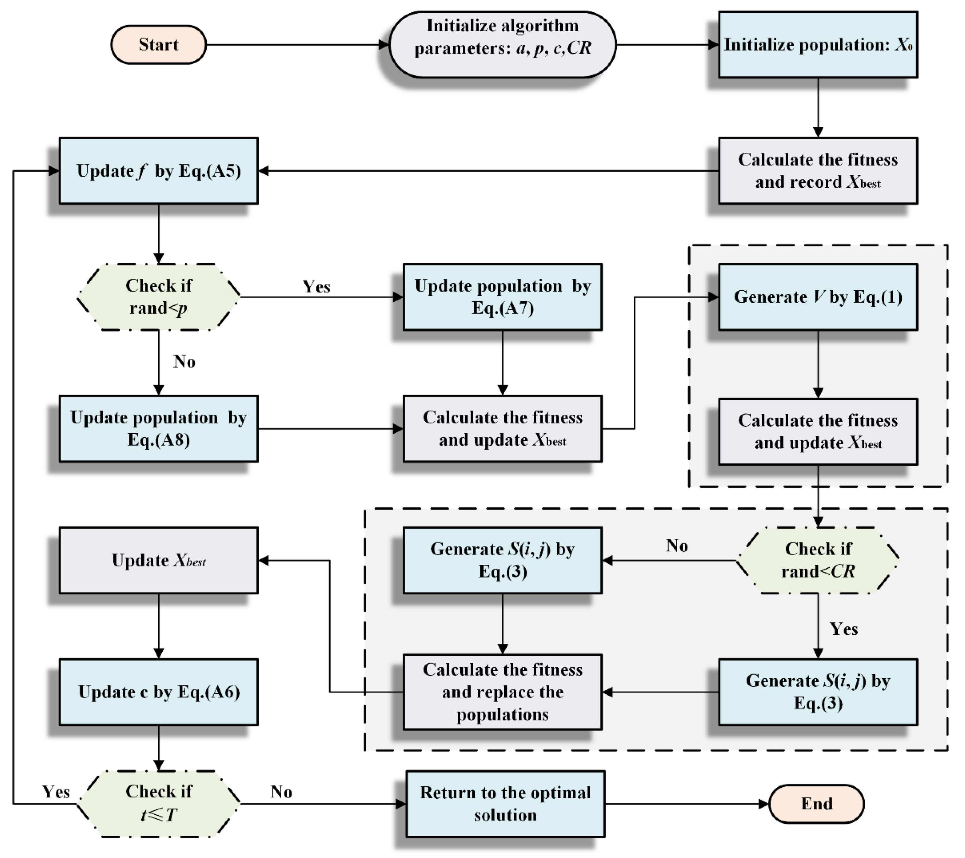
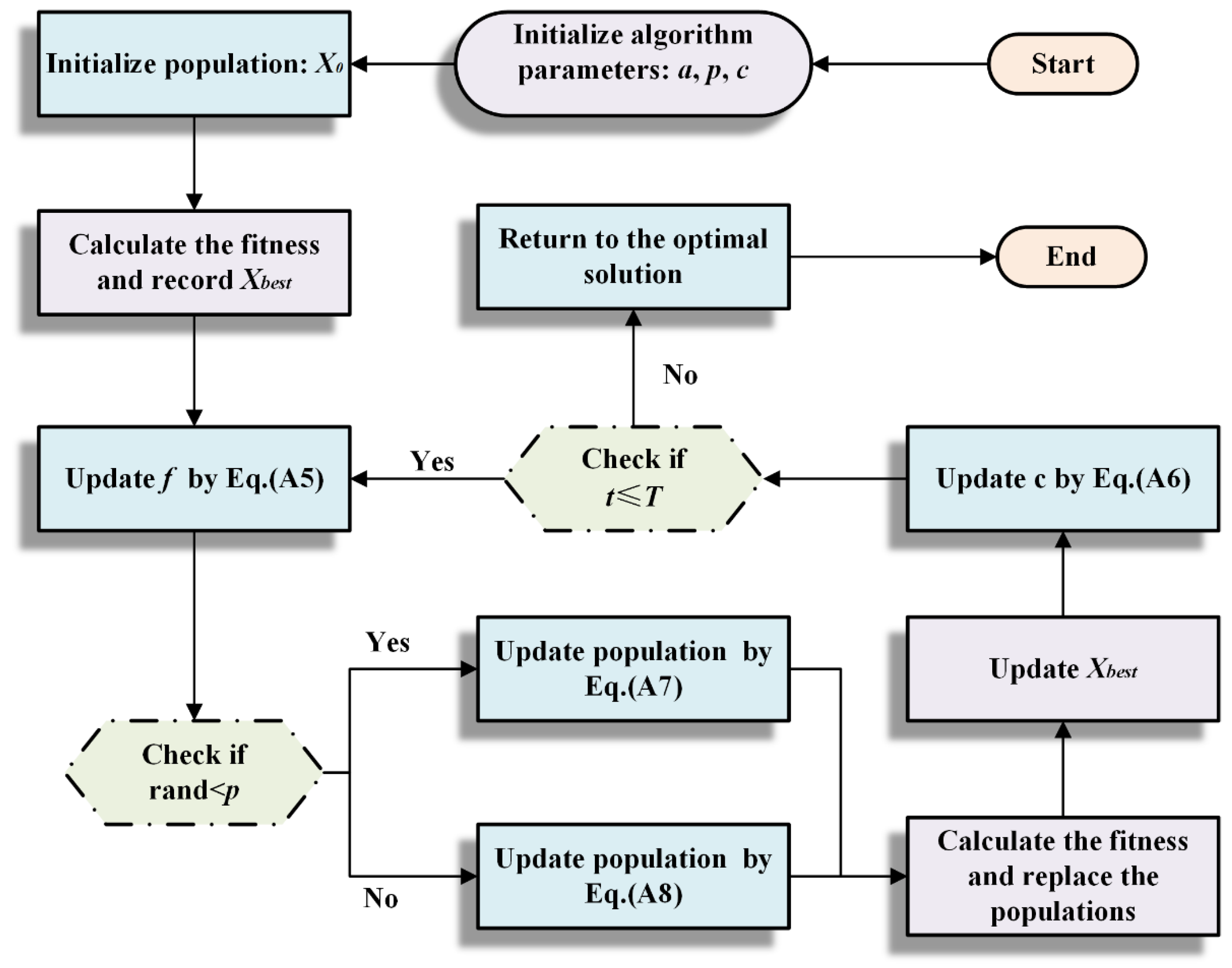
In this section, we propose CBBOA based on the above two mechanisms and introduce the entire process of CBBOA. CBBOA adds the above two mechanisms to BOA. CBBOA enters the communication mechanism stage after updating the population. Next, we use Equation (1) to generate a temporary individual V. Then, use Equation (3) to generate a temporary population S. Afterwards, it decides whether to replace the original population after comparison. Finally, we update the optimal solution; so far, a complete iteration end. Figure 1 shows the concrete process.

The temporal complexity of CBBOA is governed by the maximum number of iterations (T), the number of dimensions (dim), and the size of the population in each dimension (N). According to the results of the study, the overall time complexity of CBBOA is O(CBBOA) = O(initialization) + O(calculation fitness) + T ∗ (O(update position by BOA) + O(communication mechanism) + O(Gaussian Bare-Bones) + O(update the optimal solution)). Initializing the population has a O(N ∗ dim) time complexity, which means it takes a long time. The time complexity of computing fitness is O(N). Using BOA formula to update the time complexity is O(N). The time complexity of CM is O(N). The Gaussian Bare-Bones is O(N ∗ dim) and update the optimal solution is O(N). Therefore, its final complexity is as below. $\mathrm{O}\left(\mathrm{CBBOA}\right)=\mathrm{O}\left(N*dim\right)+\mathrm{O}\left(N\right)+T*\left(\mathrm{O}\left(N\right)+\mathrm{O}\left(N\right)+\mathrm{O}\left(N*dim\right)+\mathrm{O}\left(N\right)\right)=\mathrm{O}\left(N*dim\right)+\mathrm{O}\left(N\right)+T*\left(3\mathrm{O}\left(N\right)+\mathrm{O}\left(N*dim\right)\right)$.

3. Proposed CBBOA-SVM Method

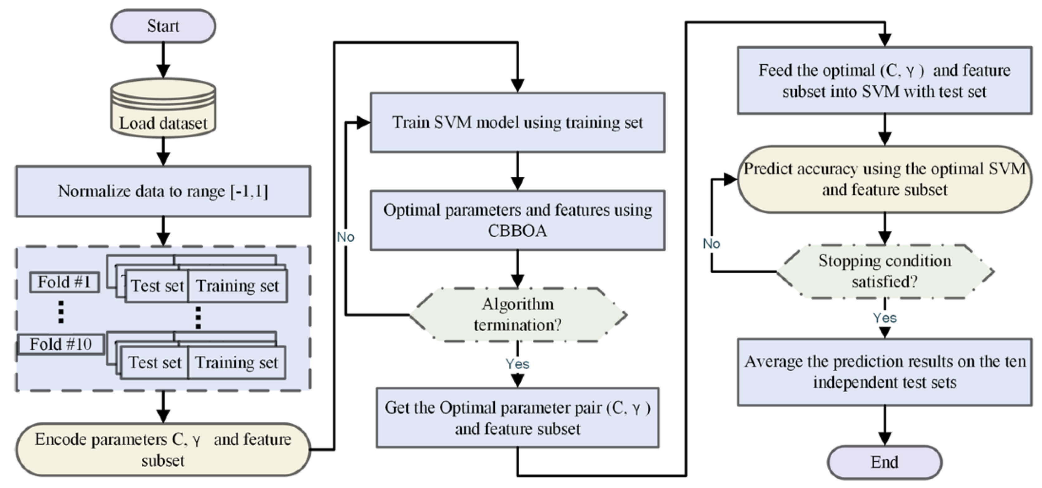
The two factors that affect the classification accuracy of SVM are the setting of hyperparameters and the selection of feature set, where the hyperparameters include penalty factor C and the kernel parameter $\gamma$, which greatly affect the classification accuracy. Feature subsets also use the entire set or a random selection, which results in low efficiency and accuracy. Based on this, we propose CBBOA-SVM to optimize the SVM by searching for the optimal hyperparameters as well as a subset of features. Next, we apply the model to two realistic scenarios to test the superiority of the model. Figure 2 depicts the framework of the CBBOA-SVM. The model consists mostly of two key components. The classification accuracy (ACC) of this optimized SVM is acquired in the right half using 10-fold cross-validation, nine of which are used to train and the remainder to test.

4. Experiments

4.1. Collection of Data

In this paper, a random web survey was conducted using Questionnaire Star to randomly select students from general undergraduate colleges and universities (comprehensive category), Sino-foreign cooperative colleges and universities, higher vocational colleges and universities (comprehensive category), and general undergraduate colleges and universities (specialist category). A total of 557 questionnaires were collected. Taking into account the volume of questions and the speed of answering, those with an answer time of 120 seconds or more were classified as valid questionnaires, totaling 445, of which 310 were male and 247 were female, and the distribution of majors included science and technology, medicine and health, literature, history and philosophy, arts, and sports. By examining the gender, education, grade, major, place of origin of the respondents, as well as the Chinese version of the Basic Psychological Needs Satisfaction Scale (nine attributes) using self-determination theory, and the Student Career Construct Questionnaire (25 attributes) (see

Table 1. Descriptions of each attribute.

Attributes	Name	Descriptions
F1	Gender	One for female, two for male
F2	Education	There are three categories: undergraduate in progress, specialist (senior) in progress, and master’s in progress, indicated by 1, 2, and 3, respectively.
F3	Grade	There are six categories: freshmen, sophomores, juniors, seniors, other grades, and graduate students, denoted by 1, 2, 3, 4, 5, and 6, respectively.
F4	Specialty	There are four categories: science and technology, literature, history and philosophy, medicine and health, and arts and sports, indicated by 1, 2, 3, and 4, respectively.
F5	Source	There are two categories, urban and rural, indicated by 1 and 2, respectively.
F6	Make choices based on interests and values	It is used to measure the degree of satisfaction of the individual’s basic psychological needs for autonomy, with higher values indicating higher satisfaction.
F7	Do things freely in your own way	Same as F6
F8	Express “ true self “ through my choice	Same as F6
F9	Successfully complete difficult tasks and programs	It is used to measure the degree of satisfaction of competence needs among the basic psychological needs of individuals, and a higher value indicates a higher degree of satisfaction.
F10	Accept and win difficult challenges	Same as F9
F11	Feel empowered by what you do	Same as F9
F12	Have a sense of connection with people who care about me and who I care about	It is used to measure the degree of satisfaction of relationship needs among the basic psychological needs of individuals, with higher values indicating higher satisfaction.
F13	Feel intimately connected to significant others	Same as F12
F14	Have a strong sense of closeness to those around you	Same as F12
F15	Have a clear understanding of the formation of self-personality traits	It is used to measure the clarity of an individual’s self-concept, with higher values indicating greater clarity.
F16	Know your natural abilities	Same as F15
F17	Decide what is more important to me (values)	Same as F15
F18	Know what others see in me	Same as F15
F19	Set an example in your mind	Same as F15
F20	Find out what I am interested in	Same as F15
F21	Set goals for yourself	Same as F15
F22	Interview with Career Professionals	It is used to measure the progress of individual career exploration, with higher values indicating better progress.
F23	Discuss your career	Same as F22
F24	Understand the type of job	Same as F22
F25	Read career information	Same as F22
F26	Research suitable careers	Same as F22
F27	Conduct career experience	Same as F22
F28	Identify the training required for the occupation	Same as F22
F29	Decide what you want to do	It is used to measure the clarity of an individual’s career decisions and goals, with higher values indicating greater clarity.
F30	Find the right job path	Same as F29
F31	Choose a career that you are satisfied with	Same as F29
F32	Develop an action plan for choosing a career	Same as F29
F33	Reconfirmation of a wise career choice	Same as F29
F34	Develop specific knowledge or skills needed for the job	It is used to measure the degree of learning of an individual’s required skills, with higher values indicating higher levels of learning.
F35	Get the training and experience you need	Same as F34
F36	Participate in the training required for the job	Same as F34
F37	Have the qualifications required for the job	Same as F34
F38	Develop a job search plan	It is used to measure an individual’s readiness for the transition from school to work, with higher values indicating greater readiness.
F39	Get a job once you complete the training	Same as F38

), the importance of these attributes and their intrinsic connections were explored, and a prediction model for college students’ career decisions was established on this basis.

4.2. Experimental Setup

The experiment was carried out with the assistance of the MATLAB R2018 software. Prior to dealing with classification, the data were scaled to [−1,1] before being analyzed.

In computational science, the fair setting of experiments plays a very important role in the comparison of methods, such as molecular signature identification [17,18], drug discovery [19,20], and recommender system [21,22,23,24]. The data was split using the k-fold cross-validation (CV) method, with the value of k being set to 10 [25,26].

5. Experimental Results

5.1. Benchmark Function Validation

This section mainly introduces and discusses related experiments to verify the performance of CBBOA. In order to verify the performance of CBBOA, we tested it with other advanced algorithms on the selected benchmark functions. In addition, in order to explore the impact of the mechanisms on CBBOA, a balance and diversity analysis experiment was also added.

5.1.1. Test Conditions and Benchmark Functions

It is important to set the fair test conditions for the comparison experiment [27,28,29,30,31]. All experiments were tested in the same environment, where the dimension, number of populations, and number of random runs were set to 30, while the maximum number of evaluations was 300,000, and CEC2014 was chosen as the test function set [32].

Table A1. Test benchmark functions.

ID	Function Equation	Dim	Range	F(min)
Unimodal Functions
F1	Rotated High Conditioned Elliptic Function	30	[−100,100]	100
F2	Rotated Bent Cigar Function	30	[−100,100]	200
F3	Rotated Discus Function	30	[−100,100]	300
Simple Multimodal Functions
F4	Shifted and Rotated Rosenbrock’s Function	30	[−100,100]	400
F5	Shifted and Rotated Ackley’s Function	30	[−100,100]	500
F6	Shifted and Rotated Weierstrass Function	30	[−100,100]	600
F7	Shifted and Rotated Griewank’s Function	30	[−100,100]	700
F8	Shifted Rastrigin’s Function	30	[−100,100]	800
F9	Shifted and Rotated Rastrigin’s Function	30	[−100,100]	900
F10	Shifted Schwefel’s Function	30	[−100,100]	1000
F11	Shifted and Rotated Schwefel’s Function	30	[−100,100]	1100
F12	Shifted and Rotated Katsuura Function	30	[−100,100]	1200
F13	Shifted and Rotated HappyCat Function	30	[−100,100]	1300
F14	Shifted and Rotated HGBat Function	30	[−100,100]	1400
F15	Shifted and Rotated Expanded Griewank’s plus Rosenbrock’s Function	30	[−100,100]	1500
F16	Shifted and Rotated Expanded Scaffer’s F6 Function	30	[−100,100]	1600
Hybrid Function
F17	Hybrid Function 1	30	[−100,100]	1700
F18	Hybrid Function 2	30	[−100,100]	1800
F19	Hybrid Function 3	30	[−100,100]	1900
F20	Hybrid Function 4	30	[−100,100]	2000
F21	Hybrid Function 5	30	[−100,100]	2100
F22	Hybrid Function 6	30	[−100,100]	2200
Composition Functions
F23	Composition Function 1	30	[−100,100]	2300
F24	Composition Function 2	30	[−100,100]	2400
F25	Composition Function 3	30	[−100,100]	2500
F26	Composition Function 4	30	[−100,100]	2600
F27	Composition Function 5	30	[−100,100]	2700
F28	Composition Function 6	30	[−100,100]	2800
F29	Composition Function 7	30	[−100,100]	2900
F30	Composition Function 8	30	[−100,100]	3000

shows the selected 30 benchmark functions which have been used in many recent studies [33,34]. In the table, the last three columns indicate the dimensionality, the upper and lower bounds of the search space, and the optimal solution of the corresponding function. In addition, the functions are divided into unimodal, simple multimodal, hybrid, and composition functions. The reason for choosing different types of functions is to evaluate the performance of the algorithm more comprehensively.

5.1.2. Comparison with the Excellent Algorithms

In order to test the effectiveness of the proposed CBBOA, several high-quality algorithms are selected for comparison with CBBOA in this section. The tested algorithms include BMWOA [35], ACWOA [36], COSCA [37], CESCA [38], CGPSO [39], ALCPSO [40], GL25 [41], DECLS [42], DE [43], GWO [44], and BOA.

Table A2. Comparison results of CBBOA and other algorithms.

	F1		F2
	Avg	Std	Avg	Std
CBBOA	1.8030 × 106	1.0304 × 106	2.0001 × 102	9.2127 × 10−3
BMWOA	1.0717 × 108	4.3745 × 107	2.6567 × 108	1.5529 × 108
ACWOA	1.4833 × 108	5.5638 × 107	7.9939 × 109	3.4474 × 109
COSCA	8.9386 × 108	5.3031 × 108	6.3658 × 1010	2.1103 × 1010
CESCA	1.1876 × 109	2.0735 × 108	7.6944 × 1010	4.2170 × 109
CGPSO	9.7702 × 106	2.5780 × 106	1.5498 × 108	2.1136 × 107
ALCPSO	6.4899 × 106	6.6766 × 106	2.2696 × 103	3.8048 × 103
GL25	6.8886 × 106	3.8457 × 106	1.2582 × 103	1.1673 × 103
DECLS	3.3217 × 107	9.1089 × 106	1.1338 × 103	3.6390 × 103
DE	1.9301 × 107	5.7413 × 106	8.2095 × 102	1.6488 × 103
GWO	5.5892 × 107	3.5683 × 107	2.1901 × 109	2.5341 × 109
BOA	1.6643 × 109	3.1079 × 108	7.8163 × 1010	8.3707 × 109
	F3		F4
	Avg	Std	Avg	Std
CBBOA	4.0850 × 102	1.3860 × 102	4.7838 × 102	3.6867 × 101
BMWOA	5.4968 × 104	9.3525 × 103	6.7336 × 102	7.3102 × 101
ACWOA	4.9095 × 104	8.8924 × 103	1.1387 × 103	2.8025 × 102
COSCA	5.6942 × 104	1.7497 × 104	9.8014 × 103	3.0534 × 103
CESCA	1.1103 × 105	1.5056 × 104	1.1600 × 104	1.4613 × 103
CGPSO	2.2727 × 103	6.6309 × 102	4.6431 × 102	3.1795 × 101
ALCPSO	5.1468 × 102	5.7009 × 102	5.1660 × 102	4.4261 × 101
GL25	7.1686 × 103	1.1124 × 104	5.1182 × 102	3.3736 × 101
DECLS	5.1436 × 102	1.8144 × 102	5.0966 × 102	1.9755 × 101
DE	4.0464 × 102	1.0122 × 102	5.0399 × 102	2.6263 × 101
GWO	3.1663 × 104	8.2882 × 103	6.4242 × 102	8.7207 × 101
BOA	7.3093 × 104	7.0422 × 103	1.6572 × 104	2.0742 × 103
	F5		F6
	Avg	Std	Avg	Std
CBBOA	5.2054 × 102	9.1124 × 10−2	6.1011 × 102	3.4478 × 100
BMWOA	5.2097 × 102	9.2063 × 10−2	6.3329 × 102	2.9235 × 100
ACWOA	5.2080 × 102	1.5647 × 10−1	6.3348 × 102	3.4412 × 100
COSCA	5.2104 × 102	7.6610 × 10−2	6.2130 × 102	4.7481 × 100
CESCA	5.2103 × 102	5.0365 × 10−2	6.4161 × 102	1.5680 × 100
CGPSO	5.2096 × 102	5.2391 × 10−2	6.2282 × 102	3.2396 × 100
ALCPSO	5.2082 × 102	6.2548 × 10−2	6.1614 × 102	3.6276 × 100
GL25	5.2107 × 102	1.2606 × 10−1	6.1431 × 102	2.9503 × 100
DECLS	5.2064 × 102	6.0533 × 10−2	6.2158 × 102	1.9812 × 100
DE	5.2057 × 102	5.7521 × 10−2	6.1966 × 102	2.0167 × 100
GWO	5.2096 × 102	5.3745 × 10−2	6.1427 × 102	2.8626 × 100
BOA	5.2105 × 102	4.2576 × 10−2	6.3918 × 102	1.5880 × 100
	F7		F8
	Avg	Std	Avg	Std
CBBOA	7.0001 × 102	1.3748 × 10−2	8.1898 × 102	1.0020 × 101
BMWOA	7.0291 × 102	8.9324 × 10−1	9.7229 × 102	2.6449 × 101
ACWOA	7.3695 × 102	1.6757 × 101	1.0027 × 103	2.4405 × 101
COSCA	1.1459 × 103	1.7911 × 102	1.0319 × 103	1.0624 × 102
CESCA	1.4151 × 103	5.7444 × 101	1.2180 × 103	1.5325 × 101
CGPSO	7.0237 × 102	1.8918 × 10−1	9.8251 × 102	2.2402 × 101
ALCPSO	7.0001 × 102	1.2223 × 10−2	8.2025 × 102	9.3172 × 100
GL25	7.0005 × 102	4.7467 × 10−2	8.5966 × 102	1.7631 × 101
DECLS	7.0000 × 102	4.9595 × 10−6	8.0092 × 102	9.9010 × 10−1
DE	7.0000 × 102	5.6014 × 10−13	8.0097 × 102	8.1531 × 10−1
GWO	7.1835 × 102	1.7971 × 101	8.8460 × 102	2.3224 × 101
BOA	1.5084 × 103	9.3231 × 101	1.0800 × 103	2.3929 × 101
	F9		F10
	Avg	Std	Avg	Std
CBBOA	9.9137 × 102	2.3780 × 101	1.6058 × 103	3.6765 × 102
BMWOA	1.1237 × 103	2.4960 × 101	4.8429 × 103	6.8002 × 102
ACWOA	1.1296 × 103	2.6544 × 101	4.8371 × 103	8.0218 × 102
COSCA	1.1912 × 103	4.7617 × 101	3.9767 × 103	7.9244 × 102
CESCA	1.3040 × 103	1.5796 × 101	8.8141 × 103	2.9668 × 102
CGPSO	1.1188 × 103	2.3346 × 101	5.5081 × 103	5.8401 × 102
ALCPSO	1.0081 × 103	3.0592 × 101	1.7183 × 103	4.3505 × 102
GL25	1.0288 × 103	3.3241 × 101	3.7255 × 103	9.2637 × 102
DECLS	1.0230 × 103	9.6967 × 100	1.0252 × 103	2.5235 × 101
DE	1.0098 × 103	9.3311 × 100	1.0301 × 103	4.1062 × 101
GWO	1.0040 × 103	2.1414 × 101	3.4005 × 103	5.9025 × 102
BOA	1.2821 × 103	4.7244 × 101	6.9291 × 103	3.9695 × 102
	F11		F12
	Avg	Std	Avg	Std
CBBOA	5.0119 × 103	6.0250 × 102	1.2009 × 103	2.3915 × 10−1
BMWOA	7.1530 × 103	6.0590 × 102	1.2024 × 103	4.8900 × 10−1
ACWOA	6.4025 × 103	8.5223 × 102	1.2018 × 103	4.4736 × 10−1
COSCA	6.3104 × 103	6.1537 × 102	1.2020 × 103	4.1068 × 10−1
CESCA	9.1132 × 103	2.4588 × 102	1.2036 × 103	4.0427 × 10−1
CGPSO	6.0632 × 103	4.8645 × 102	1.2026 × 103	2.3568 × 10−1
ALCPSO	4.1988 × 103	6.6139 × 102	1.2015 × 103	4.8177 × 10−1
GL25	6.4044 × 103	6.7616 × 102	1.2025 × 103	8.3770 × 10−1
DECLS	6.1820 × 103	2.5230 × 102	1.2011 × 103	1.3085 × 10−1
DE	5.8411 × 103	3.0834 × 102	1.2009 × 103	1.2453 × 10−1
GWO	3.9793 × 103	9.0198 × 102	1.2019 × 103	1.0066 × 100
BOA	7.6936 × 103	3.0339 × 102	1.2029 × 103	3.7932 × 10−1
	F13		F14
	Avg	Std	Avg	Std
CBBOA	1.3004 × 103	8.5067 × 10−2	1.4002 × 103	3.4669 × 10−2
BMWOA	1.3006 × 103	1.5480 × 10−1	1.4003 × 103	4.3141 × 10−2
ACWOA	1.3015 × 103	1.0365 × 100	1.4191 × 103	1.5916 × 101
COSCA	1.3057 × 103	2.6847 × 100	1.6137 × 103	8.0522 × 101
CESCA	1.3078 × 103	4.8390 × 10−1	1.6506 × 103	2.2394 × 101
CGPSO	1.3004 × 103	1.0740 × 10−1	1.4003 × 103	1.1888 × 10−1
ALCPSO	1.3005 × 103	8.7747 × 10−2	1.4007 × 103	3.0709 × 10−1
GL25	1.3004 × 103	8.0749 × 10−2	1.4003 × 103	5.0502 × 10−2
DECLS	1.3004 × 103	6.2113 × 10−2	1.4003 × 103	8.7249 × 10−2
DE	1.3004 × 103	4.2062 × 10−2	1.4003 × 103	4.5312 × 10−2
GWO	1.3004 × 103	1.0651 × 10−1	1.4028 × 103	5.0769 × 100
BOA	1.3088 × 103	3.9353 × 10−1	1.6981 × 103	3.5360 × 101
	F15		F16
	Avg	Std	Avg	Std
CBBOA	1.5098 × 103	2.5115 × 100	1.6113 × 103	6.4364 × 10−1
BMWOA	1.5759 × 103	4.1733 × 101	1.6125 × 103	3.2151 × 10−1
ACWOA	2.0604 × 103	6.0202 × 102	1.6120 × 103	5.3325 × 10−1
COSCA	3.6836 × 105	1.6560 × 105	1.6125 × 103	3.8935 × 10−1
CESCA	4.3189 × 105	1.0374 × 105	1.6135 × 103	2.1406 × 10−1
CGPSO	1.5174 × 103	1.1700 × 100	1.6115 × 103	3.5374 × 10−1
ALCPSO	1.5095 × 103	3.1903 × 100	1.6117 × 103	5.2657 × 10−1
GL25	1.5220 × 103	6.9231 × 100	1.6120 × 103	5.0226 × 10−1
DECLS	1.5133 × 103	8.2274 × 10−1	1.6118 × 103	2.8453 × 10−1
DE	1.5121 × 103	9.6677 × 10−1	1.6115 × 103	2.9432 × 10−1
GWO	2.1591 × 103	1.3597 × 103	1.6108 × 103	6.5913 × 10−1
BOA	3.8960 × 105	1.3187 × 105	1.6134 × 103	2.8382 × 10−1
	F17		F18
	Avg	Std	Avg	Std
CBBOA	2.1792 × 105	1.2091 × 105	3.9527 × 103	2.1688 × 103
BMWOA	5.5900 × 106	3.7204 × 106	8.5449 × 104	6.4288 × 104
ACWOA	1.6134 × 107	1.0735 × 107	5.0025 × 107	3.6272 × 107
COSCA	3.0648 × 107	3.5516 × 107	7.1814 × 108	2.1449 × 109
CESCA	1.0504 × 108	1.8015 × 107	4.0499 × 109	9.6455 × 108
CGPSO	3.1879 × 105	1.2726 × 105	2.8501 × 106	6.4288 × 105
ALCPSO	4.7325 × 105	5.4772 × 105	8.3538 × 103	7.5279 × 103
GL25	8.2784 × 105	4.6405 × 105	2.7815 × 103	1.4342 × 103
DECLS	2.0297 × 106	8.4694 × 105	1.9452 × 104	1.6845 × 104
DE	1.5640 × 106	6.5718 × 105	8.6163 × 103	4.8731 × 103
GWO	2.6886 × 106	2.9678 × 106	6.2481 × 106	1.4825 × 107
BOA	1.7617 × 108	8.5409 × 107	6.4244 × 109	2.5330 × 109
	F19		F20
	Avg	Std	Avg	Std
CBBOA	1.9123 × 103	1.6232 × 101	3.6498 × 103	1.2646 × 103
BMWOA	1.9331 × 103	2.3707 × 101	3.1152 × 104	2.7581 × 104
ACWOA	2.0086 × 103	2.9753 × 101	4.1432 × 104	1.9260 × 104
COSCA	2.0930 × 103	2.0199 × 102	2.5987 × 104	9.0261 × 103
CESCA	2.2572 × 103	4.4261 × 101	4.4640 × 105	2.8889 × 105
CGPSO	1.9177 × 103	2.8220 × 100	2.4449 × 103	8.9684 × 101
ALCPSO	1.9132 × 103	1.5071 × 101	3.0207 × 103	5.0969 × 102
GL25	1.9177 × 103	1.8849 × 101	1.5454 × 104	9.4537 × 103
DECLS	1.9090 × 103	1.1062 × 100	5.5417 × 103	1.9236 × 103
DE	1.9083 × 103	7.1246 × 10−1	4.9888 × 103	1.5815 × 103
GWO	1.9421 × 103	2.6740 × 101	1.8691 × 104	9.2334 × 103
BOA	2.4468 × 103	7.1856 × 101	1.3607 × 105	1.0837 × 105
	F21		F22
	Avg	Std	Avg	Std
CBBOA	1.5122 × 105	9.4180 × 104	2.5175 × 103	1.4193 × 102
BMWOA	1.7781 × 106	1.7201 × 106	2.8403 × 103	2.1005 × 102
ACWOA	5.3323 × 106	4.3368 × 106	2.9696 × 103	2.3798 × 102
COSCA	4.2385 × 105	4.1713 × 105	2.5624 × 103	1.3627 × 102
CESCA	3.6023 × 107	1.1128 × 107	5.6077 × 103	1.2488 × 103
CGPSO	1.7853 × 105	1.1978 × 105	2.9412 × 103	2.1692 × 102
ALCPSO	6.5221 × 104	6.3401 × 104	2.6419 × 103	2.3292 × 102
GL25	2.4524 × 105	1.5452 × 105	2.5479 × 103	1.2323 × 102
DECLS	3.4290 × 105	1.7048 × 105	2.4056 × 103	8.5474 × 101
DE	2.9194 × 105	1.4617 × 105	2.3745 × 103	9.1063 × 101
GWO	5.7270 × 105	1.3318 × 106	2.5510 × 103	1.7590 × 102
BOA	6.5589 × 107	6.2651 × 107	2.9678 × 104	2.4451 × 104
	F23		F24
	Avg	Std	Avg	Std
CBBOA	2.6152 × 103	1.1517 × 10−12	2.6000 × 103	5.1366 × 10−13
BMWOA	2.5006 × 103	9.7621 × 10−1	2.6003 × 103	2.8177 × 10−1
ACWOA	2.5187 × 103	5.7177 × 101	2.6000 × 103	1.9497 × 10−6
COSCA	2.5000 × 103	0.0000 × 100	2.6000 × 103	1.4417 × 10−4
CESCA	3.1011 × 103	1.1310 × 102	2.6559 × 103	2.1852 × 101
CGPSO	2.5000 × 103	1.6453 × 10−3	2.6000 × 103	1.2108 × 10−2
ALCPSO	2.6153 × 103	2.6885 × 10−2	2.6317 × 103	1.2483 × 101
GL25	2.6152 × 103	5.4858 × 10−11	2.6348 × 103	7.6871 × 100
DECLS	2.5000 × 103	1.5125 × 10−3	2.6000 × 103	1.1092 × 10−2
DE	2.6152 × 103	1.3876 × 10−12	2.6266 × 103	2.9836 × 100
GWO	2.6348 × 103	8.6286 × 100	2.6000 × 103	6.9708 × 10−4
BOA	2.5000 × 103	0.0000 × 100	2.6000 × 103	4.9958 × 10−13
	F25		F26
	Avg	Std	Avg	Std
CBBOA	2.7000 × 103	0.0000 × 100	2.7568 × 103	5.0205 × 101
BMWOA	2.7000 × 103	7.5052 × 10−3	2.7006 × 103	1.4230 × 10−1
ACWOA	2.7000 × 103	0.0000 × 100	2.7570 × 103	5.0001 × 101
COSCA	2.7000 × 103	0.0000 × 100	2.7535 × 103	5.0524 × 101
CESCA	2.7173 × 103	7.7569 × 100	2.7126 × 103	1.3655 × 100
CGPSO	2.7000 × 103	4.5423 × 10−5	2.7900 × 103	3.0386 × 101
ALCPSO	2.7112 × 103	3.5602 × 100	2.7659 × 103	8.0123 × 101
GL25	2.7149 × 103	3.2778 × 100	2.7470 × 103	5.0602 × 101
DECLS	2.7000 × 103	2.8374 × 10−5	2.7003 × 103	6.4985 × 10−2
DE	2.7070 × 103	1.0605 × 100	2.7003 × 103	3.7748 × 10−2
GWO	2.7093 × 103	4.8242 × 100	2.7635 × 103	4.8781 × 101
BOA	2.7000 × 103	0.0000 × 100	2.7710 × 103	3.9722 × 101
	F27		F28
	Avg	Std	Avg	Std
CBBOA	3.2793 × 103	1.4039 × 102	3.8798 × 103	1.9790 × 102
BMWOA	2.9001 × 103	1.6129 × 10−1	3.0002 × 103	2.0453 × 10−1
ACWOA	3.7057 × 103	3.4813 × 102	3.6620 × 103	1.0791 × 103
COSCA	2.9168 × 103	6.4131 × 101	3.0000 × 103	0.0000 × 100
CESCA	3.9890 × 103	1.7575 × 102	5.4311 × 103	3.3799 × 102
CGPSO	2.9750 × 103	1.8597 × 102	3.1379 × 103	7.5511 × 102
ALCPSO	3.4654 × 103	2.3066 × 102	4.3818 × 103	4.7586 × 102
GL25	3.2986 × 103	1.1776 × 102	4.0664 × 103	2.1919 × 102
DECLS	3.0343 × 103	1.8568 × 102	3.0442 × 103	1.6814 × 102
DE	3.2247 × 103	1.0311 × 102	3.6416 × 103	2.4955 × 101
GWO	3.3653 × 103	1.2923 × 102	3.9109 × 103	2.0234 × 102
BOA	3.2618 × 103	8.1426 × 101	9.4775 × 103	9.0608 × 102
	F29		F30
	Avg	Std	Avg	Std
CBBOA	2.3085 × 106	3.9835 × 106	6.0232 × 103	1.0071 × 103
BMWOA	9.2623 × 105	2.7754 × 106	5.0326 × 104	4.0784 × 104
ACWOA	2.4172 × 107	2.4069 × 107	4.1810 × 105	3.6525 × 105
COSCA	3.4284 × 106	1.0796 × 107	4.6562 × 104	1.2930 × 105
CESCA	1.7522 × 107	3.5720 × 106	1.3828 × 106	3.1673 × 105
CGPSO	6.3314 × 103	2.7923 × 103	1.3065 × 104	1.0994 × 104
ALCPSO	1.2267 × 106	3.7342 × 106	1.2522 × 104	8.6766 × 103
GL25	4.1844 × 103	2.1535 × 102	6.7032 × 103	8.8310 × 102
DECLS	6.6570 × 103	9.6293 × 103	6.6640 × 103	1.2451 × 103
DE	5.0815 × 103	1.8380 × 103	6.2438 × 103	1.1828 × 103
GWO	1.3376 × 106	3.5286 × 106	5.2609 × 104	3.5890 × 104
BOA	3.1000 × 103	0.0000 × 100	3.2000 × 103	5.9714 × 10−5

records the experimental results of CBBOA and the above algorithms on the CEC14 function.

In the table, Avg represents the average result, and Std represents the standard deviation. The best performing results on each function in the table have been bolded. We can see nine of the results of CBBOA ranking first. In the F1~F16, CBBOA ranks in the top three out of 15 functions. On F17~F30, which have more complicated function structures, CBBOA ranks in the top three among the nine functions. In contrast, the original BOA only performed well in F23, F24, and F25, and ranked at the end among other functions. This shows that the improvement for BOA is effective. CBBOA can achieve good results on different kinds of functions. These functions are more comprehensive and more versatile.

In order to analyze the experimental results more comprehensively, we used the Wilcoxon signed-rank test [45] to analyze the experimental results. In the Wilcoxon signed-rank test, when the p-value is less than 0.05, it indicates that this algorithm has a significant improvement compared with another algorithm in statistics.

Table A3. The p-value of CBBOA versus other algorithms.

	BMWOA	ACWOA	COSCA	CESCA	CGPSO	ALCPSO
F1	1.7344 × 10−6	1.7344 × 10−6	1.7344 × 10−6	1.7344 × 10−6	1.7344 × 10−6	2.8308 × 10−4
F2	1.7344 × 10−6	1.7344 × 10−6	1.7344 × 10−6	1.7344 × 10−6	1.7344 × 10−6	2.1266 × 10−6
F3	1.7344 × 10−6	1.7344 × 10−6	1.7344 × 10−6	1.7344 × 10−6	1.7344 × 10−6	1.5286 × 10−1
F4	1.7344 × 10−6	1.7344 × 10−6	1.7344 × 10−6	1.7344 × 10−6	9.3676 × 10−2	5.3197 × 10−3
F5	1.7344 × 10−6	3.8822 × 10−6	1.7344 × 10−6	1.7344 × 10−6	1.7344 × 10−6	1.7344 × 10−6
F6	1.7344 × 10−6	1.7344 × 10−6	1.7344 × 10−6	1.7344 × 10−6	2.3534 × 10−6	1.6394 × 10−5
F7	1.7344 × 10−6	1.7344 × 10−6	1.7344 × 10−6	1.7344 × 10−6	1.7344 × 10−6	5.0085 × 10−1
F8	1.7344 × 10−6	1.7344 × 10−6	1.7344 × 10−6	1.7344 × 10−6	1.7344 × 10−6	9.7539 × 10−1
F9	1.7344 × 10−6	1.7344 × 10−6	1.7344 × 10−6	1.7344 × 10−6	1.7344 × 10−6	7.5213 × 10−2
F10	1.7344 × 10−6	1.7344 × 10−6	1.7344 × 10−6	1.7344 × 10−6	1.7344 × 10−6	2.7116 × 10−1
F11	1.9209 × 10−6	9.3157 × 10−6	3.5152 × 10−6	1.7344 × 10−6	5.7517 × 10−6	6.8923 × 10−5
F12	1.9209 × 10−6	1.7344 × 10−6	1.9209 × 10−6	1.7344 × 10−6	1.7344 × 10−6	3.8811 × 10−4
F13	5.7517 × 10−6	1.7344 × 10−6	1.9209 × 10−6	1.7344 × 10−6	8.6121 × 10−1	5.3070 × 10−5
F14	1.4773 × 10−4	1.7344 × 10−6	1.7344 × 10−6	1.7344 × 10−6	4.4052 × 10−1	1.9209 × 10−6
F15	1.7344 × 10−6	1.7344 × 10−6	1.7344 × 10−6	1.7344 × 10−6	1.7344 × 10−6	9.0993 × 10−1
F16	2.6033 × 10−6	4.4493 × 10−5	2.3534 × 10−6	1.7344 × 10−6	3.0010 × 10−2	4.3896 × 10−3
F17	1.7344 × 10−6	1.7344 × 10−6	1.7344 × 10−6	1.7344 × 10−6	7.7309 × 10−3	7.5213 × 10−2
F18	1.7344 × 10−6	1.7344 × 10−6	1.7344 × 10−6	1.7344 × 10−6	1.7344 × 10−6	1.7088 × 10−3
F19	2.0515 × 10−4	1.7344 × 10−6	3.5152 × 10−6	1.7344 × 10−6	3.5888 × 10−4	1.1093 × 10−1
F20	1.7344 × 10−6	1.7344 × 10−6	1.7344 × 10−6	1.7344 × 10−6	4.7292 × 10−6	3.0010 × 10−2
F21	2.1266 × 10−6	1.7344 × 10−6	4.8603 × 10−5	1.7344 × 10−6	5.9994 × 10−1	5.2872 × 10−4
F22	1.2381 × 10−5	2.1266 × 10−6	2.2888 × 10−1	1.7344 × 10−6	1.9209 × 10−6	1.9569 × 10−2
F23	1.7322 × 10−6	2.9944 × 10−7	4.3205 × 10−8	1.7322 × 10−6	1.7322 × 10−6	1.7333 × 10−6
F24	1.7344 × 10−6	6.8988 × 10−5	1.1914 × 10−1	1.7344 × 10−6	1.7344 × 10−6	2.1253 × 10−6
F25	1.7333 × 10−6	1.0000 × 100	1.0000 × 100	1.7333 × 10−6	1.7333 × 10−6	1.7344 × 10−6
F26	2.2545 × 10−3	1.8408 × 10−1	9.1082 × 10−1	3.6085 × 10−3	7.5137 × 10−5	8.9718 × 10−2
F27	1.7344 × 10−6	4.0715 × 10−5	1.7344 × 10−6	1.7344 × 10−6	4.8603 × 10−5	7.7122 × 10−4
F28	1.7344 × 10−6	2.6230 × 10−1	1.7344 × 10−6	1.7344 × 10−6	3.1123 × 10−5	6.3198 × 10−5
F29	5.5774 × 10−1	3.7243 × 10−5	2.7653 × 10−3	1.7344 × 10−6	3.7094 × 10−1	1.8462 × 10−1
F30	2.1266 × 10−6	7.6909 × 10−6	3.8203 × 10−1	1.7344 × 10−6	1.7518 × 10−2	1.6394 × 10−5
	GL25	DECLS	DE	GWO	BOA
F1	1.9209 × 10−6	1.7344 × 10−6	1.7344 × 10−6	1.7344 × 10−6	1.7344 × 10−6
F2	1.7344 × 10−6	3.3173 × 10−4	3.6094 × 10−3	1.7344 × 10−6	1.7344 × 10−6
F3	1.7344 × 10−6	9.8421 × 10−3	8.7740 × 10−1	1.7344 × 10−6	1.7344 × 10−6
F4	1.1138 × 10−3	4.1955 × 10−4	3.8542 × 10−3	1.9209 × 10−6	1.7344 × 10−6
F5	1.9209 × 10−6	3.4053 × 10−5	2.2888 × 10−1	1.7344 × 10−6	1.7344 × 10−6
F6	3.8811 × 10−4	1.7344 × 10−6	2.1266 × 10−6	2.8308 × 10−4	1.7344 × 10−6
F7	1.6046 × 10−4	1.4093 × 10−4	1.5391 × 10−4	1.7344 × 10−6	1.7344 × 10−6
F8	1.7344 × 10−6	1.7333 × 10−6	1.9185 × 10−6	1.9209 × 10−6	1.7344 × 10−6
F9	8.9187 × 10−5	1.9729 × 10−5	6.6392 × 10−4	1.1093 × 10−1	1.7344 × 10−6
F10	1.7344 × 10−6	1.9209 × 10−6	1.9209 × 10−6	1.7344 × 10−6	1.7344 × 10−6
F11	2.1266 × 10−6	2.6033 × 10−6	5.2165 × 10−6	4.0715 × 10−5	1.7344 × 10−6
F12	1.7344 × 10−6	1.0357 × 10−3	1.2544 × 10−1	2.8434 × 10−5	1.7344 × 10−6
F13	8.1302 × 10−1	1.6503 × 10−1	1.8519 × 10−2	5.8571 × 10−1	1.7344 × 10−6
F14	1.2453 × 10−2	1.6394 × 10−5	3.5152 × 10−6	4.0715 × 10−5	1.7344 × 10−6
F15	1.7344 × 10−6	2.1630 × 10−5	4.5336 × 10−4	1.7344 × 10−6	1.7344 × 10−6
F16	2.5967 × 10−5	1.6046 × 10−4	1.2544 × 10−1	4.9498 × 10−2	1.7344 × 10−6
F17	2.3534 × 10−6	1.7344 × 10−6	1.7344 × 10−6	3.5152 × 10−6	1.7344 × 10−6
F18	4.2767 × 10−2	2.3534 × 10−6	1.8910 × 10−4	2.3704 × 10−5	1.7344 × 10−6
F19	7.7122 × 10−4	2.8021 × 10−1	8.4508 × 10−1	1.9209 × 10−6	1.7344 × 10−6
F20	1.7344 × 10−6	4.1955 × 10−4	5.7064 × 10−4	1.7344 × 10−6	1.7344 × 10−6
F21	1.2453 × 10−2	1.7988 × 10−5	1.1499 × 10−4	7.8647 × 10−2	1.7344 × 10−6
F22	5.8571 × 10−1	7.7122 × 10−4	4.1955 × 10−4	5.3044 × 10−1	1.7344 × 10−6
F23	1.6354 × 10−6	1.7344 × 10−6	1.0000 × 100	1.7344 × 10−6	4.3205 × 10−8
F24	1.7333 × 10−6	1.7333 × 10−6	1.7333 × 10−6	1.7333 × 10−6	6.2500 × 10−2
F25	1.7333 × 10−6	1.7333 × 10−6	1.7333 × 10−6	1.2279 × 10−5	1.0000 × 100
F26	5.0383 × 10−1	2.3704 × 10−5	1.9729 × 10−5	1.0937 × 10−1	8.5924 × 10−2
F27	6.5833 × 10−1	3.4053 × 10−5	2.0589 × 10−1	3.3269 × 10−2	6.4352 × 10−1
F28	1.2866 × 10−3	1.7344 × 10−6	1.7344 × 10−6	5.4401 × 10−1	1.7344 × 10−6
F29	3.0650 × 10−4	1.3591 × 10−1	8.2206 × 10−2	2.8948 × 10−1	1.7344 × 10−6
F30	1.3194 × 10−2	2.4308 × 10−2	4.1653 × 10−1	1.7344 × 10−6	1.7344 × 10−6

shows the p-value of CBBOA compared with other algorithms. Values greater than or equal to 0.05 are indicated in bold. From the table, we can see that CBBOA has improved significantly over CESCA in all functions. Compared with BMWOA, it can be found that only one function has a test value not less than 0.05. Compared with the original BOA, CBBOA has significant improvements in functions other than F24~F27. This once again proves that the performance of CBBOA is superior and more comprehensive.

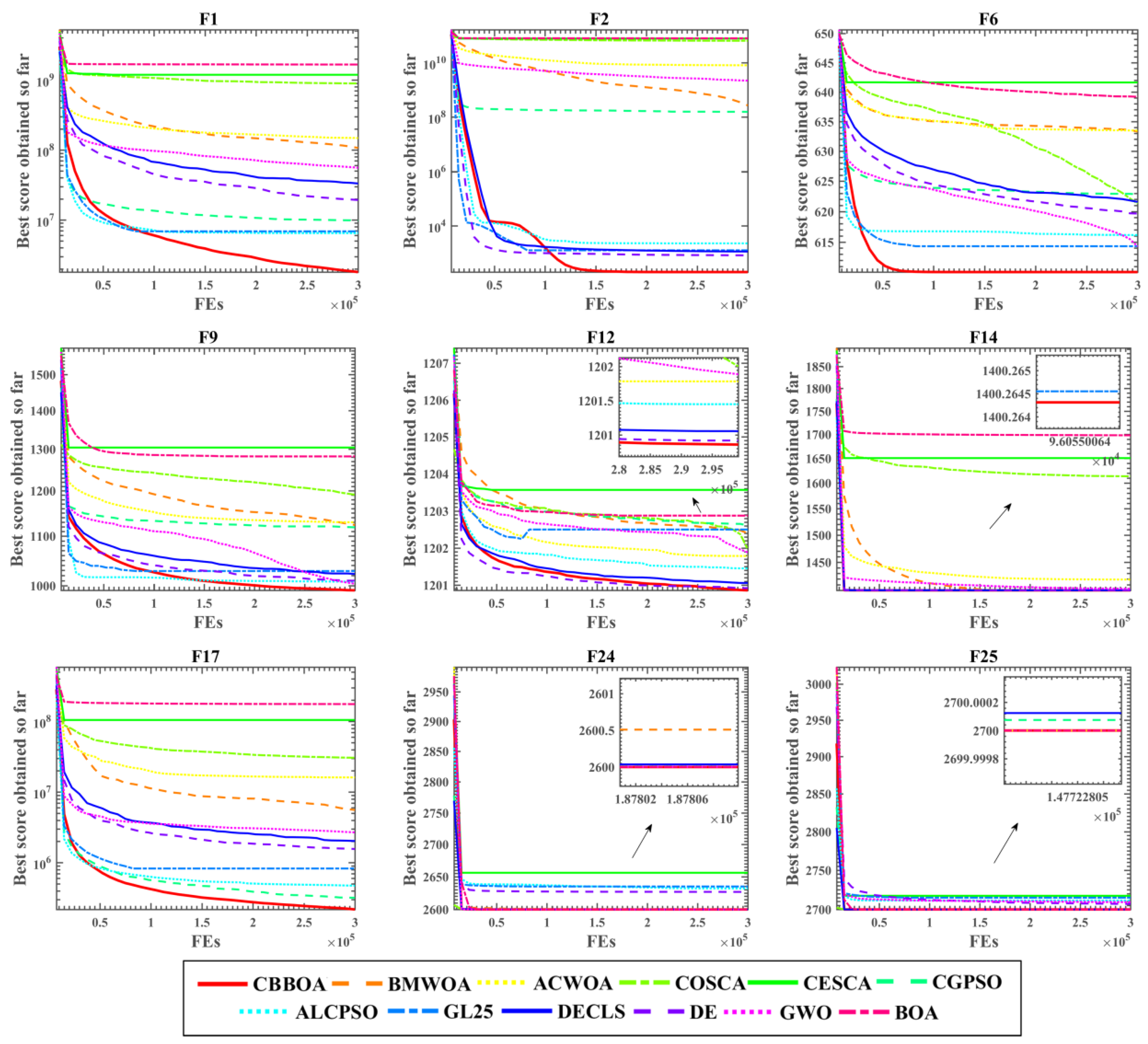
The convergence curves of this experiment can be seen in Figure 3. From the figure, we can see that in F1, F2, F6, and F17, the convergence curve of CBBOA has obvious advantages. In F9, algorithms such as ALCPSO and GL25 have stabilized in the early stage of iteration, while CBBOA can continue to decline. This shows that CBBOA doesn’t easily fall into the local optimum. This is where CBBOA has improved compared with BOA.

5.1.3. Mechanism Comparison Experiment

We made a mechanism comparison experiment to compare the effects of the two mechanisms added in CBBOA. To compare the effects of the two mechanisms, we set up an algorithm that uses only a single mechanism, hence the following four algorithms are used for testing: CBBOA, BOABB, BOACM, and BOA. BOABB means that the original BOA adds Gaussian Bare-Bones. BOACM only adds a communication mechanism. CBBOA added both mechanisms. BOA is the original version. The four algorithms are tested on the same 30 benchmark functions.

Table A4. Comparison results of CBBOA and other algorithms.

	F1			F2
	Avg	Std		Avg	Std
CBBOA	1.4818 × 106	7.6067 × 105	CBBOA	2.0000 × 102	8.9172 × 10−3
BOABB	2.1815 × 106	1.1008 × 106	BOABB	2.0000 × 102	3.7543 × 10−3
BOACM	1.4030 × 109	2.0120 × 108	BOACM	7.6129 × 1010	1.0019 × 1010
BOA	1.7705 × 109	2.9979 × 108	BOA	7.5017 × 1010	6.8016 × 109
	F3			F4
	Avg	Std		Avg	Std
CBBOA	4.1096 × 102	1.2917 × 102	CBBOA	4.7678 × 102	3.7929 × 101
BOABB	4.5098 × 102	1.6666 × 102	BOABB	4.8281 × 102	3.7593 × 101
BOACM	7.6585 × 104	4.3189 × 103	BOACM	1.3699 × 104	3.0500 × 103
BOA	7.4196 × 104	5.6359 × 103	BOA	1.6618 × 104	2.1750 × 103
	F5			F6
	Avg	Std		Avg	Std
CBBOA	5.2052 × 102	9.0294 × 10−2	CBBOA	6.1162 × 102	3.4318 × 100
BOABB	5.2050 × 102	7.6702 × 10−2	BOABB	6.1223 × 102	3.0495 × 100
BOACM	5.2100 × 102	5.8757 × 10−2	BOACM	6.3825 × 102	1.7127 × 100
BOA	5.2105 × 102	6.0785 × 10−2	BOA	6.3823 × 102	2.2752 × 100
	F7			F8
	Avg	Std		Avg	Std
CBBOA	7.0001 × 102	1.3063 × 10−2	CBBOA	8.1958 × 102	7.8919 × 100
BOABB	7.0001 × 102	1.1507 × 10−2	BOABB	8.2585 × 102	1.0404 × 101
BOACM	1.3306 × 103	8.9903 × 101	BOACM	1.0957 × 103	2.1952 × 101
BOA	1.5138 × 103	6.5163 × 101	BOA	1.0867 × 103	2.8582 × 101
	F9			F10
	Avg	Std		Avg	Std
CBBOA	9.9045 × 102	2.9712 × 101	CBBOA	1.5833 × 103	2.9764 × 102
BOABB	9.7194 × 102	2.1876 × 101	BOABB	1.6668 × 103	3.8606 × 102
BOACM	1.2604 × 103	1.8657 × 101	BOACM	6.9789 × 103	3.5990 × 102
BOA	1.2788 × 103	3.3273 × 101	BOA	6.8713 × 103	4.0484 × 102
	F11			F12
	Avg	Std		Avg	Std
CBBOA	4.6879 × 103	7.0222 × 102	CBBOA	1.2008 × 103	1.9694 × 10−1
BOABB	5.0674 × 103	7.8285 × 102	BOABB	1.2008 × 103	2.1869 × 10−1
BOACM	7.5830 × 103	5.1201 × 102	BOACM	1.2028 × 103	3.1569 × 10−1
BOA	7.5866 × 103	3.4520 × 102	BOA	1.2028 × 103	4.2705 × 10−1
	F13			F14
	Avg	Std		Avg	Std
CBBOA	1.3004 × 103	6.5511 × 10−2	CBBOA	1.4002 × 103	3.9803 × 10−2
BOABB	1.3004 × 103	6.4113 × 10−2	BOABB	1.4003 × 103	1.0610 × 10−1
BOACM	1.3084 × 103	7.9012 × 10−1	BOACM	1.6396 × 103	2.4950 × 101
BOA	1.3088 × 103	6.0851 × 10−1	BOA	1.6987 × 103	2.9022 × 101
	F15			F16
	Avg	Std		Avg	Std
CBBOA	1.5085 × 103	2.6655 × 100	CBBOA	1.6112 × 103	4.8598 × 10−1
BOABB	1.5093 × 103	2.9331 × 100	BOABB	1.6113 × 103	4.3135 × 10−1
BOACM	1.5791 × 105	5.9606 × 104	BOACM	1.6128 × 103	2.6040 × 10−1
BOA	3.6709 × 105	1.3770 × 105	BOA	1.6134 × 103	1.8603 × 10−1
	F17			F18
	Avg	Std		Avg	Std
CBBOA	2.4572 × 105	1.6260 × 105	CBBOA	3.7389 × 103	2.3791 × 103
BOABB	2.6297 × 105	1.2144 × 105	BOABB	4.4248 × 103	2.6027 × 103
BOACM	1.6116 × 108	7.3356 × 107	BOACM	5.6867 × 109	2.4342 × 109
BOA	2.1369 × 108	1.0842 × 108	BOA	6.6090 × 109	1.9399 × 109
	F19			F20
	Avg	Std		Avg	Std
CBBOA	1.9117 × 103	1.5060 × 101	CBBOA	4.1870 × 103	1.5712 × 103
BOABB	1.9148 × 103	2.0418 × 101	BOABB	4.3564 × 103	1.8372 × 103
BOACM	2.3700 × 103	8.8841 × 101	BOACM	1.8488 × 105	5.1230 × 105
BOA	2.4259 × 103	6.0800 × 101	BOA	1.1590 × 105	7.4029 × 104
	F21			F22
	Avg	Std		Avg	Std
CBBOA	9.6956 × 104	6.6030 × 104	CBBOA	2.4939 × 103	1.4941 × 102
BOABB	1.2602 × 105	1.2720 × 105	BOABB	2.4979 × 103	1.2878 × 102
BOACM	4.9917 × 107	4.5993 × 107	BOACM	3.3284 × 104	6.0774 × 104
BOA	4.8587 × 107	2.6658 × 107	BOA	4.7721 × 104	8.5557 × 104
	F23			F24
	Avg	Std		Avg	Std
CBBOA	2.6037 × 103	3.5164 × 101	CBBOA	2.6000 × 103	5.9711 × 10−13
BOABB	2.6152 × 103	1.5548 × 10−12	BOABB	2.6064 × 103	1.0767 × 101
BOACM	2.5000 × 103	0.0000 × 100	BOACM	2.6000 × 103	8.4444 × 10−14
BOA	2.5000 × 103	0.0000 × 100	BOA	2.6000 × 103	4.4684 × 10−13
	F25			F26
	Avg	Std		Avg	Std
CBBOA	2.7000 × 103	0.0000 × 100	CBBOA	2.7602 × 103	4.9627 × 101
BOABB	2.7000 × 103	0.0000 × 100	BOABB	2.7116 × 103	4.6443 × 101
BOACM	2.7000 × 103	0.0000 × 100	BOACM	2.7714 × 103	3.8205 × 101
BOA	2.7000 × 103	0.0000 × 100	BOA	2.7733 × 103	3.8978 × 101
	F27			F28
	Avg	Std		Avg	Std
CBBOA	3.2691 × 103	1.2932 × 102	CBBOA	3.8365 × 103	1.3805 × 102
BOABB	3.2718 × 103	1.5141 × 102	BOABB	3.8623 × 103	1.9048 × 102
BOACM	2.9598 × 103	6.6784 × 101	BOACM	3.6505 × 103	1.4264 × 103
BOA	3.2628 × 103	7.4755 × 101	BOA	8.9360 × 103	8.8515 × 102
	F29			F30
	Avg	Std		Avg	Std
CBBOA	3.0868 × 106	4.5614 × 106	CBBOA	6.2096 × 103	8.9321 × 102
BOABB	2.6707 × 106	3.6263 × 106	BOABB	6.6561 × 103	2.0851 × 103
BOACM	3.1000 × 103	0.0000 × 100	BOACM	3.2000 × 103	3.7537 × 10−5
BOA	3.1000 × 103	0.0000 × 100	BOA	7.3943 × 103	2.2973 × 104

records the experimental results. Similarly, the best-optimized solution for each function is bolded. In the table, we can see that among 30 functions, CBBOA ranks first in 19 functions. In addition to comparing Avg, comparing the values of Std can prove that CBBOA is more stable than other algorithms. This shows that the combination of the two mechanisms exerts a better effect.

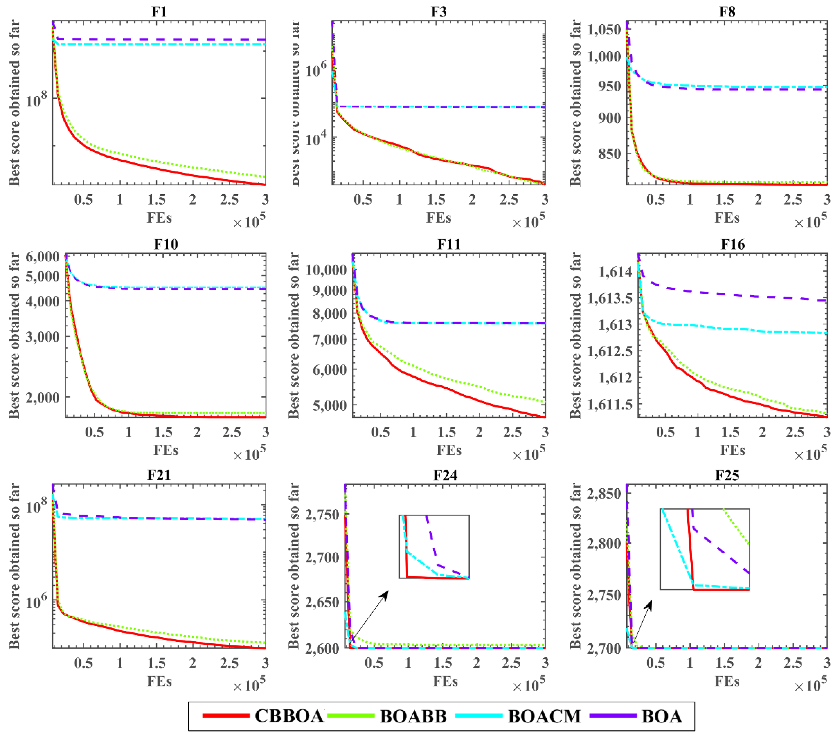
Figure 4 shows the convergence curves of the above experiment. In F1 and F11, we can clearly see that CBBOA has got a better solution. We can see that the optimal solutions of the four algorithms are relatively similar in F24 and F25. However, the convergence speed of CBBOA is faster than BOABB and BOA in these two functions. The above experimental analyses all show that the combination of the two mechanisms helps BOA achieve better performance.

5.1.4. Qualitative Analysis

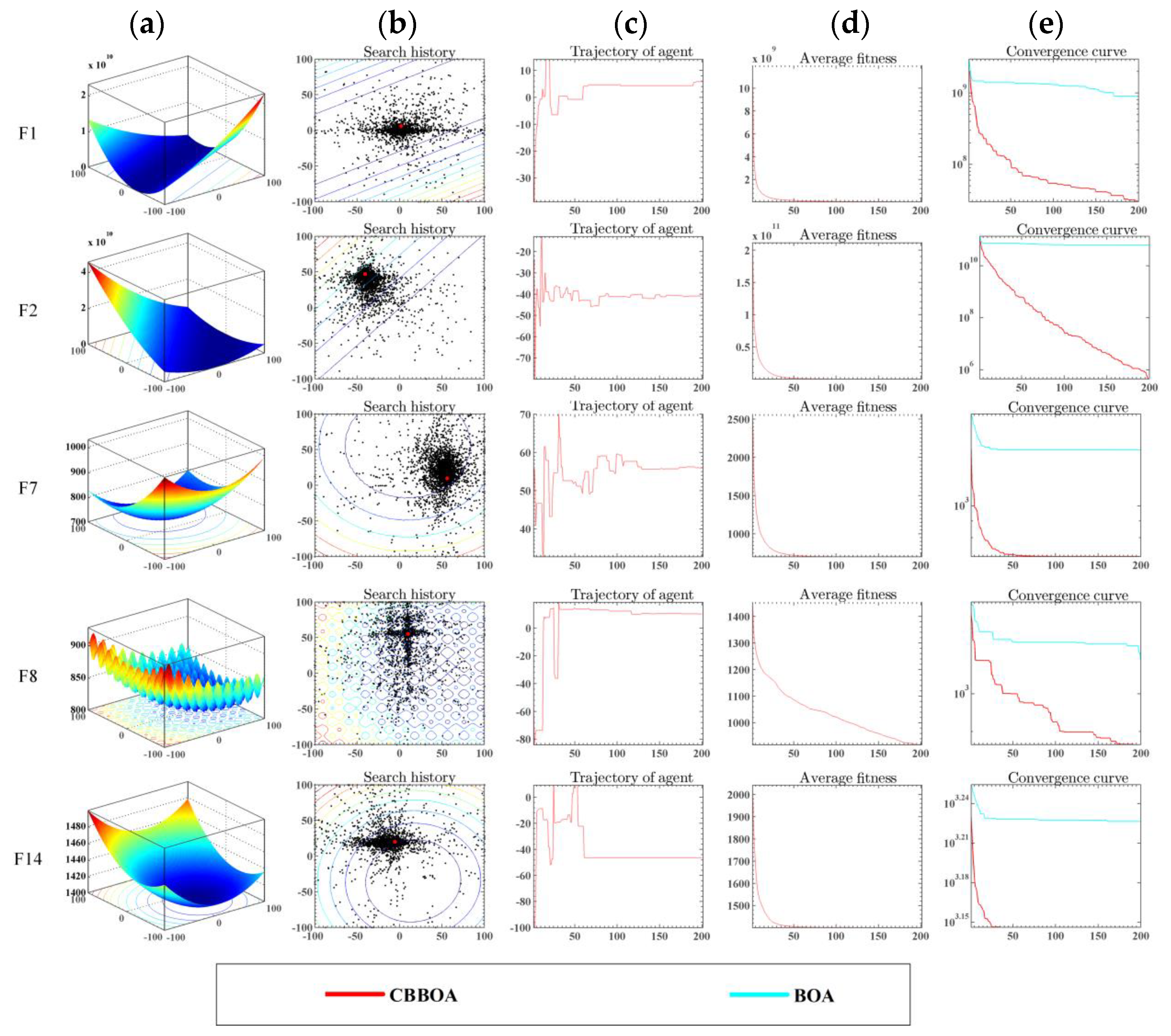
The purpose of this part is to undertake a qualitative study of CBBOA. In the first instance, the function of CEC14 is subjected to a feasibility study. The findings of the feasibility study of CBBOA and BOA are shown in Figure 5. In the illustration, there are five columns. The figure shows five columns of data, from left to right, indicating the three-dimensional distribution, two-dimensional distribution, and one-dimensional distribution of the search trajectory of CBBOA in the multidimensional space, the variation of the average fitness, and the convergence curve, respectively. In Figure 5b, the red dot shows the position of the optimum solution, and the black dot represents the location of the search for CBBOA, which is shown in the lower right corner. The fact that the black dots are dispersed over the whole search plane in the picture indicates that CBBOA is capable of traversing the solution space to the greatest extent conceivable. The black dots closest to the best answer are the densest, indicating that CBBOA can define the target region and perform additional development in this part of the world. The trajectory curve in Figure 5c fluctuates greatly in the early period and tends to stabilize in the later period. The fluctuation of the trajectory indicates that the algorithm is searching extensively in the early period. When the algorithm finds the target area, the trajectory becomes stable. In Figure 5d, the average fitness decreases during the iteration. The average fitness dropped to a lower value in the mid-term, indicating that the CBBOA has a good convergence speed. In Figure 5e, the convergence curve of CBBOA is lower than BOA. This shows that the quality of the solutions found by CBBOA is better.

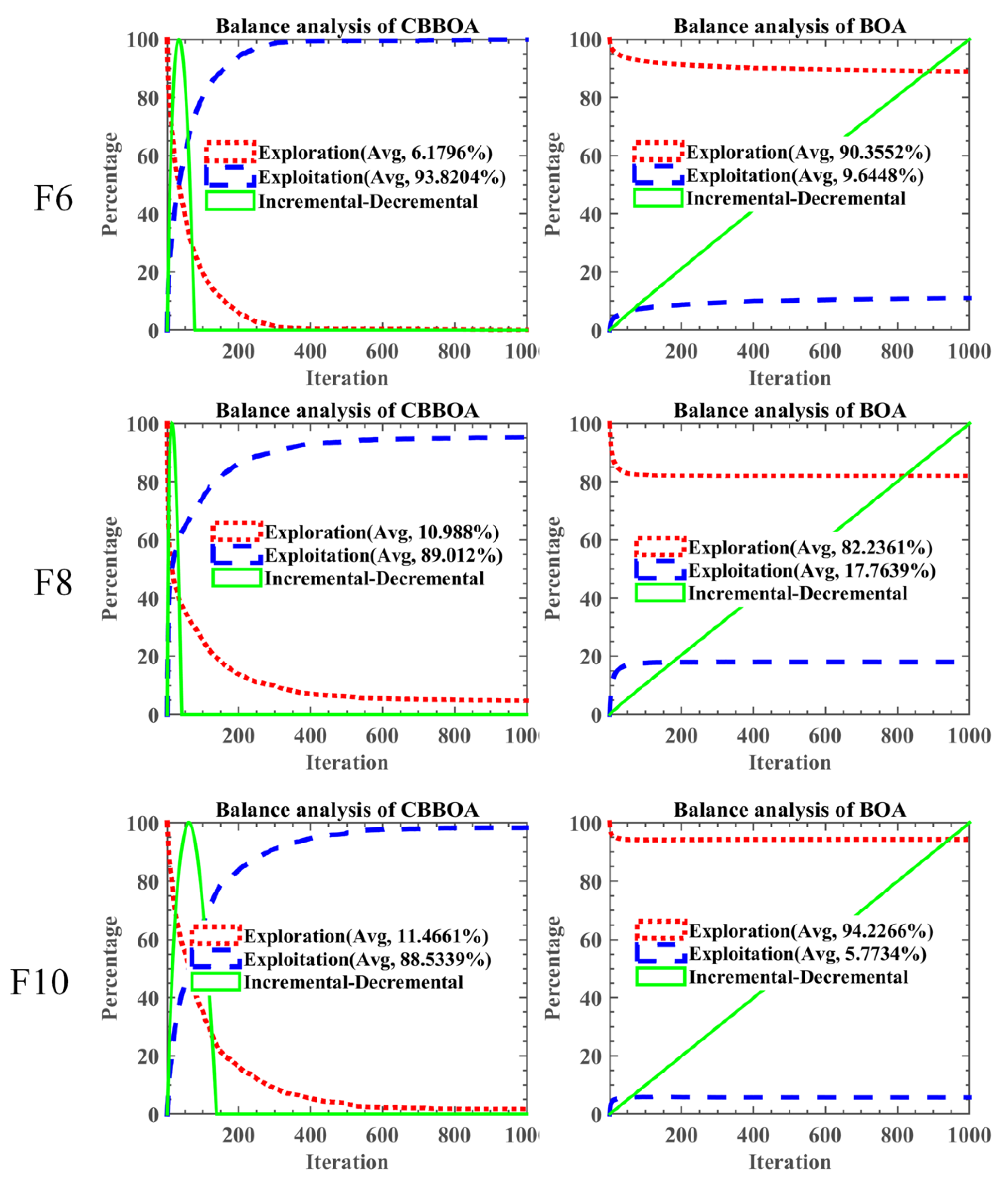
Figure 6 shows the results of the balanced analysis of CBBOA and BOA, tested on the same functions as the diversity analysis above. The results show the presence of three curves, red, blue, and green, in each graph. Red indicates the exploration capability of the algorithm, blue indicates the exploitation capability, while green is the increment–decrement curve, which is used to describe the trend of the red and blue curves, with the curve rising, indicating the dominance of exploration. On the contrary, exploitation behavior dominates. From the figure, we can see that the two behaviors are at the same level when the incremental-decremental curve reaches the maximum.

From the selected graphs, we can see that the added mechanisms have a great influence on the balance of the original BOA. The original BOA maintains a high exploration and low exploitation trend in functions. However, from the proportion of the two behaviors, we can see that the proportion of BOA exploration behavior is too high. For example, in F10, exploration accounts for more than 90%. This may lead to BOA not being able to get a high-quality solution. In contrast, the exploitation behavior of CBBOA accounts for a higher proportion. It means that it spends most of its time exploiting the target area.

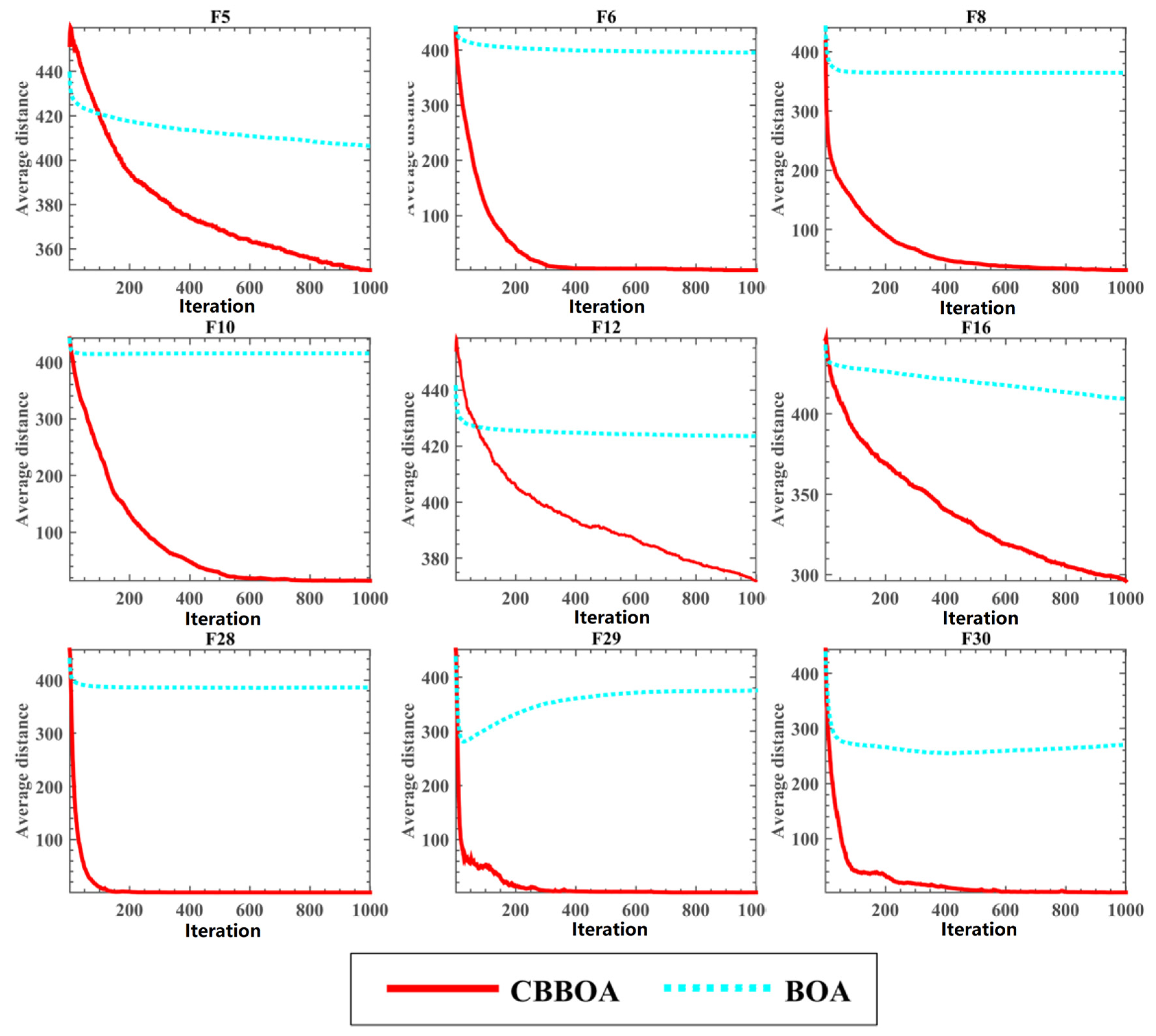
Figure 7 is the result of the diversity analysis. From the figure we can see that the diversity curves are all decreasing curves. The reason is that the algorithm randomly generates the population at the beginning, so the diversity at the beginning is large. In the process of algorithm iteration, the continuous narrowing of the search range makes the population diversity continue to decrease. As can be seen from Figure 7, the population diversity of BOA is maintained at a high value in multiple functions. This shows that BOA has been kept in a large search range and cannot determine the target area, which makes the algorithm sometimes unable to find high-quality solutions. The diversity of CBBOA can maintain a steady decline, indicating that it has determined the region where the optimal solution is located and further developed.

5.2. Predicting Results of Employment Stability

In this subsection, to investigate the impact of career decisions, we evaluated CBBOA-SVM with feature selection (CBBOA-SVM-FS) with some real datasets collected. The results of the evaluation using accuracy (ACC), Matthews Correlation Coefficient (MCC), Sensitivity, and Specificity are given in

Table 2. Classification results of CBBOA-SVM-FS in the light of four metrics.

Fold	ACC	MCC	Sensitivity	Specificity
Num.1	0.950	0.905	0.900	1.000
Num.2	0.952	0.909	0.909	1.000
Num.3	0.952	0.908	1.000	0.900
Num.4	0.952	0.909	0.909	1.000
Num.5	0.952	0.908	1.000	0.900
Num.6	0.857	0.716	0.909	0.800
Num.7	0.905	0.826	0.818	1.000
Num.8	0.950	0.905	1.000	0.900
Num.9	0.950	0.905	1.000	0.900
Num.10	1.000	1.000	1.000	1.000
AVG	0.942	0.889	0.945	0.940
STD	0.037	0.074	0.064	0.070

. The ACC of a model is defined as the proportion of properly categorized events out of all classified events, and it represents the model’s performance in categorizing the information. Specificity is a performance metric used to evaluate the ability of a binary classification model to distinguish between normal and abnormal cases. The sensitivity of the binary classification model is used to evaluate the metrics of the model in terms of spotting aberrant data. In order to properly examine the effectiveness of the classification model, the MCC is utilized. This provides a more objective predictive evaluation than just percentile rankings. Among the results given, the ACC result for CBBOA-SVM-FS is 94.2%, the MCC result is 88.9%, the Sensitivity result is 94.5%, and the Specificity result is 94%. The analysis of the results obtained by CBBOA-SVM-FS through these four evaluation metrics fully illustrates the feasibility of using CBBOA-SVM-FS to study the impact of career decisions for college students.

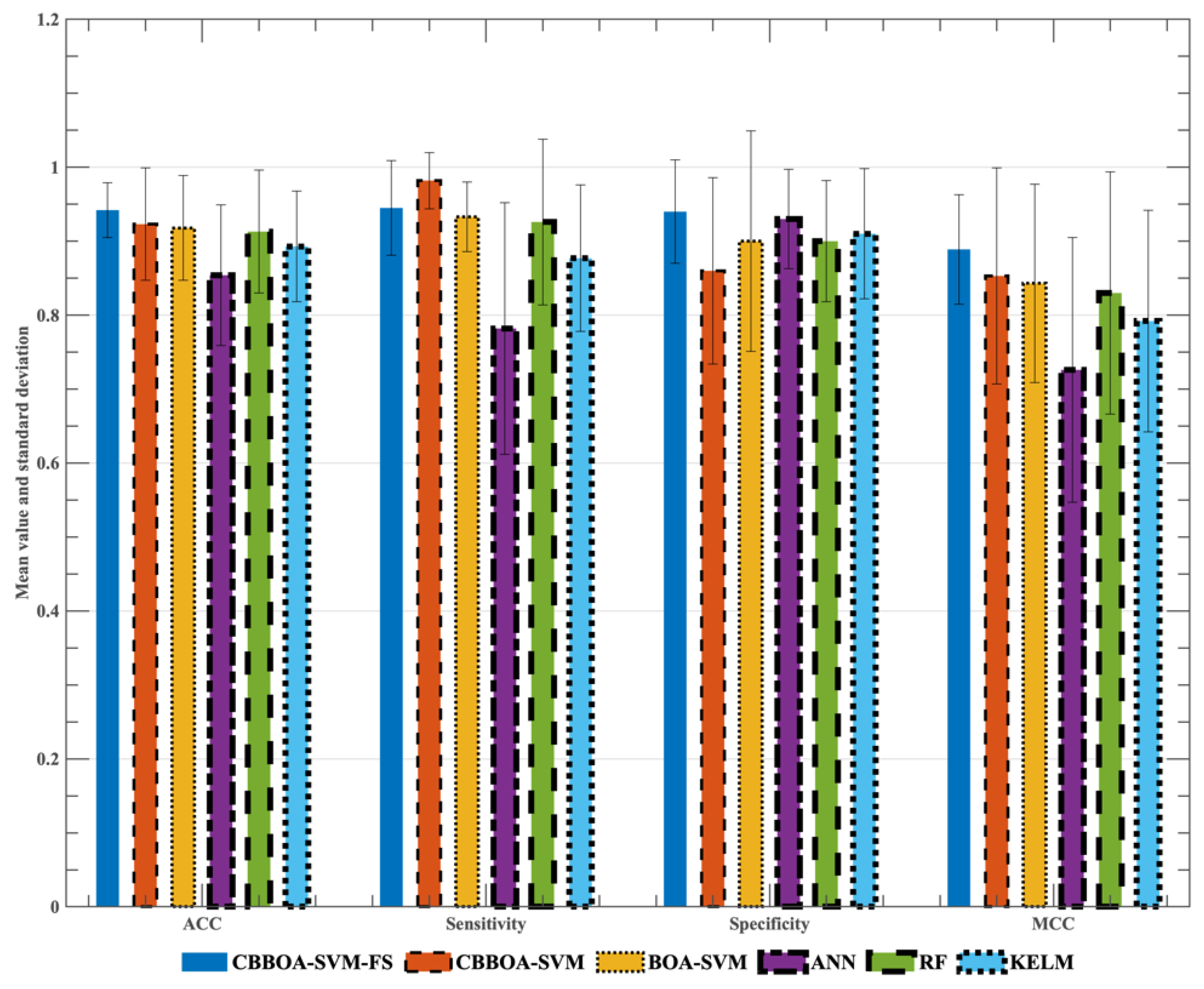
To further validate the performance of CBBOA-SVM-FS, we compared it with five other similar methods, namely CBBOA-SVM, BOA-SVM, ANN, RF, and KELM. The evaluation results of ACC, sensitivity, specificity, and MCC for each method are shown in Figure 8. For the most important one, ACC, CBBOA-SVM-FS obtained a high result of 94.20%, which is 1.90% better than CBBOA-SVM, 2.40% better than BOA-SVM, 8.80% better than ANN, 2.90% better than RF, and 4.90% better than KELM. Therefore, CBBOA-SVM-FS is the best among the performance of all the methods involved in the comparison.

Moreover, in terms of the variance of the ACC obtained by the methods involved in the comparison, CBBOA-SVM-FS is 0.037, CBBOA-SVM is 0.076, BOA-SVM is 0.071, ANN is 0.095, RF is 0.083, and KELM is 0.075. By comparing the variance, we can find that the stability of CBBOA-SVM-FS is also better with respect to ACC.

In terms of sensitivity, CBBOA-SVM obtains the best result of 98.20%, and CBBOA-SVM-FS is the second-best, with a result of 94.50%. In addition, the results of other methods are 93.30% for BOA-SVM, 92.60% for RF, 87.70% for KELM, and 78.20% for ANN, respectively, which shows that the proposed methods CBBOA-SVM-FS and CBBOA-SVM are also superior to other methods in terms of Sensitivity.

Further, the results in terms of variance also show that CBBOA-SVM-FS and CBBOA-SVM are more stable than the other methods. When evaluated using Specificity, CBBOA-SVM-FS is 94%, which is 8.00% better than CBBOA-SVM, 4.00% better than BOA-SVM, 1.00% better than ANN, 4.00% better than RF, and 3.00% better than KELM, showing that CBBOA-SVM-FS is the best. Moreover, on top of stability, CBBOA-SVM-FS is also better than CBBOA-SVM, BOA-SVM, RF, and KELM.

In the MCC results, CBBOA-SVM-FS is the best with 88.90%. CBBOA-SVM, BOA-SVM, ANN, RF, and KELM are 85.30%, 84.30%, 72.60%, 83.00%, and 79.20%, respectively, which shows that CBBOA-SVM-FS is 3.60% better than the next best CBBOA-SVM and 16.30% better than the worst ANN. Therefore, CBBOA-SVM-FS also performs the best, and its stability performance can be seen from Figure 8 that it is the best. In summary, CBBOA-SVM-FS has a better performance than other similar methods and can be used to study the impact of career decisions.

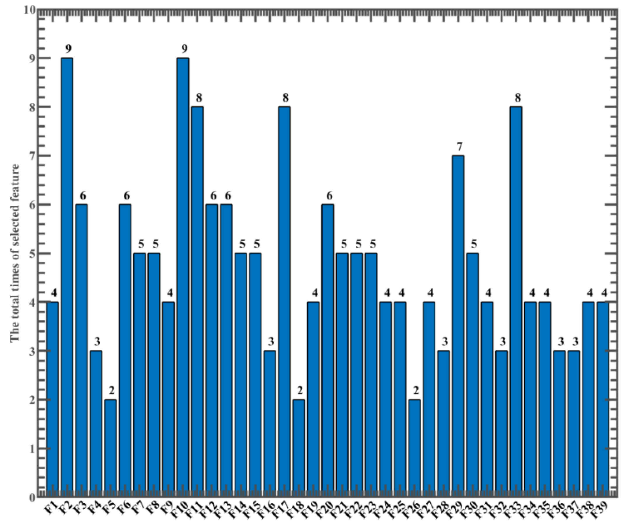
The proposed CBBOA not only accomplishes the optimum configuration of the SVM’s super parameters but also achieves the selection of the best feature set throughout the process. We took use of a ten-fold CV approach to our benefit. Figure 9 depicts the frequency distribution of the primary features found by the CBBOA-SVM via the 10-fold CV method, as determined by the CBBOA-SVM.

Because of this, as seen in the chart, the characteristics that appeared the most frequently were “Education” (F2), “Accept and win difficult challenges” (F10), “Feel empowered by what you do” (F11), “Decide what is more important to me” (values) (F17), “Set an example in your mind” (F19), “Decide what you want to do” (F29), and “Reconfirmation of a wise career choice” (F33). The five most frequent characteristics appeared 9, 9, 8, 7, and 8 times, respectively. As a result, the study came to the conclusion that such attributes may have an important role in predicting the effect of career decisions.

6. Discussion

By analyzing the results obtained experimentally for the questionnaire, it can be found that the most important 6 attribute features among the 39 attributes are F2, F10, F11, F17, F29, and F33, which have a more prominent impact on the career decision-making ability of college students.

The survey data shows that the strengths and weaknesses of college students’ career decisions differ among different education levels, with students with master’s degrees being stronger than those with bachelor’s degrees, and those with bachelor’s degrees being stronger than those with college (higher vocational), and it can be seen that the higher the education level, the stronger their career decision-making ability. This is because college students with strong career decision-making abilities have clearer and more targeted goals and clearer directions for their studies and future development, and they are more committed to improving their education.

F10 and F11 are two characteristics that measure the degree of satisfaction of competence needs among the basic psychological needs of individuals. We can find that college students who have accepted and won difficult challenges and feel competent in what they do have stronger career decision-making ability, because individuals whose competence needs are satisfied to have more confidence in their abilities in various aspects, and this ability also includes career decision-making ability. At the same time, the successes and difficulties won in career decision making promote the individual’s sense of competence.

The characteristics of F17 reflect the values in the individual’s self-concept, and it can be seen that the clearer the university students are about their self-values, the stronger their career decision-making ability is. This is because values are the overall evaluation of the meaning, role, effect, and importance of objective things (including people, things, and events) and the results of one’s own behavior, and they are the principles and standards that drive and guide one’s decisions and actions, and they are one of the core elements of the psychological structure of personality. The clearer one’s values are, the clearer one is about what one wants, needs, and needs, and the clearer and more determined one’s decisions will be; therefore, the clarity of one’s values also determines the strength of one’s career decision-making ability. We find that the stronger the degree of deciding what you want to do, the clearer the career decisions and goals, and the stronger the career decision-making ability, because deciding what to do and how to do it is part of the decision-making ability.

F33 is actually a reconfirmation and re-enforcement of the individual’s decision, which can be said to be a recognition of self-decision-making ability and can enhance the individual’s self-efficacy for decision making. The research still needs to be improved: first, the number of samples collected for the model construction needs to be increased, so that it is more comprehensive, perfect, and accurate for the model construction. Secondly, the sample collection is currently concentrated in one city, which will be influenced by factors such as the urban environment and college environment. It is necessary to expand different geographical areas, especially different provinces, to expand colleges and universities in different cities including first-tier cities, new first-tier cities, second-tier, third-tier, and fourth-tier cities, and to expand different types of colleges and universities to enrich the model. Thirdly, we can also expand more attributes that affect college students’ career decision-making ability and seek more influential attributes to make the model more convincing.

The practical value of this paper’s study on forecasting college students’ career selections is vast, and it not only can aid jobless college students in selecting acceptable occupations for themselves but also help the government’s macro-management of college students’ employment market. As a result, conducting prediction studies on college students’ future profession choices can provide very valuable information.

Because the proposed CBBOA in this paper has a strong optimization ability, it can be applied to many other scenarios in the future, such as disease module identification [46,47], molecular signatures identification for cancer diagnosis [48,49], drug-disease associations prediction [50], fractional-order controller [51], prediction of mortality rates in high-risk diabetic foot patients [52], urban road planning [53] and fault diagnosis [54,55], information retrieval services [56,57,58], and location-based services [59,60]. In addition, the method proposed in this paper can also be extended to distributed version [61,62], multi-objective or many optimization version [63,64,65], or matrix-based evolutionary computation version [66].

7. Conclusions and Future Work

In this study, we developed an effective hybrid CBBOA-SVM model to predict career decisions for college students. This paper proposes an improved BOA called CBBOA by introducing the Gaussian Bare-Bones and communication mechanism. The mechanisms effectively improve the exploitation ability and convergence accuracy of BOA. In order to evaluate the performance of CBBOA, we test it with other algorithms on benchmark functions of CEC14. Experimental results show that CBBOA has a great improvement in most functions compared with BOA. CBBOA also has competitiveness compared with some advanced algorithms. Meanwhile, by optimizing SVM with CBBOA, it is feasible to get better parameter combinations and feature subsets than previous approaches. Compared to previous machine learning approaches, the suggested method can still predict more correctly and realize more consistently while dealing with the issue of predicting career selections for college students.

In the following study, due to the advanced characteristic of the proposed CBBOA-SVM model, it will be generalized in China and utilized to anticipate various issues, such as medical diagnostics and financial risk prediction. Furthermore, it is envisaged that the CBBOA method may be expanded to handle new application domains, such photovoltaic cell optimization and optimization of deep learning network nodes.

References

- Wakelin-Theron, N.; Spowart, J. Determining tourism graduate employability, knowledge, skills, and competencies in a VUCA world: Constructing a tourism employability model. Afr. J. Hosp. Tour. Leis. 2019, 8, 1–18. [Google Scholar]
- Deci, E.L.; Ryan, R.M. Intrinsic Motivation and Self-Determination in Human Behavior; Springer Science & Business Media: New York, NY, USA, 2013. [Google Scholar]
- Rigby, C.S.; Ryan, R.M. Self-determination theory in human resource development: New directions and practical considerations. Adv. Dev. Hum. Resour. 2018, 20, 133–147. [Google Scholar] [CrossRef]
- Deci, E.L.; Olafsen, A.H.; Ryan, R.M. Self-determination theory in work organizations: The state of a science. Annu. Rev. Organ. Psychol. Organ. Behav. 2017, 4, 19–43. [Google Scholar] [CrossRef]
- Powers, K.; Chen, H.; Prasad, K.; Gilmartin, S.; Sheppard, S. Exploring How Engineering Internships and Undergraduate Research Experiences Inform and Influence College Students’ Career Decisions and Future Plans. In Proceedings of the American Society for Engineering Education Annual Conference, Salt Lake City, UT, USA, 24–27 June 2018. [Google Scholar]
- Kim, S.-Y.; Ahn, T.; Fouad, N. Family influence on Korean students’ career decisions: A social cognitive perspective. J. Career Assess. 2016, 24, 513–526. [Google Scholar] [CrossRef]
- Kiselev, P.; Kiselev, B.; Matsuta, V.; Feshchenko, A.; Bogdanovskaya, I.; Kosheleva, A. Career guidance based on machine learning: Social networks in professional identity construction. Procedia Comput. Sci. 2020, 169, 158–163. [Google Scholar] [CrossRef]
- Chung, J.Y.; Lee, S. Dropout early warning systems for high school students using machine learning. Child. Youth Serv. Rev. 2019, 96, 346–353. [Google Scholar] [CrossRef]
- Luo, T.; So, W.W.M.; Wan, Z.H.; Li, W.C. STEM stereotypes predict students’ STEM career interest via self-efficacy and outcome expectations. Int. J. STEM Educ. 2021, 8, 36. [Google Scholar] [CrossRef]
- Nauta, M.M.; Saucier, A.M.; Woodard, L.E. Interpersonal influences on students’ academic and career decisions: The impact of sexual orientation. Career Dev. Q. 2001, 49, 352–362. [Google Scholar] [CrossRef]
- Park, I.-J.; Rie, J.; Kim, H.S.; Park, J. Effects of a future time perspective–based career intervention on career decisions. J. Career Dev. 2020, 47, 96–110. [Google Scholar] [CrossRef]
- Lee, P.C.; Lee, M.J.; Dopson, L.R. Who influences college students’ career choices? An empirical study of hospitality management students. J. Hosp. Tour. Educ. 2019, 31, 74–86. [Google Scholar] [CrossRef] [Green Version]
- Tu, J.; Chen, H.; Liu, J.; Heidari, A.A.; Zhang, X.; Wang, M.; Ruby, R.; Pham, Q.-V. Evolutionary biogeography-based whale optimization methods with communication structure: Towards measuring the balance. Knowl.-Based Syst. 2021, 212, 106642. [Google Scholar] [CrossRef]
- Kennedy, J. Bare Bones Particle Swarms. In Proceedings of the 2003 IEEE Swarm Intelligence Symposium, Indianapolis, IN, USA, 26 April 2003; pp. 80–87. [Google Scholar] [CrossRef]
- Omran, M.; Engelbrecht, A.; Salman, A. Bare bones differential evolution. Eur. J. Oper. Res. 2009, 196, 128–139. [Google Scholar] [CrossRef] [Green Version]
- Wang, H.; Rahnamayan, S.; Sun, H.; Omran, M. Gaussian Bare-Bones Differential Evolution. IEEE Trans. Cybern. 2013, 43, 634–647. [Google Scholar] [CrossRef]
- Fu, J.; Zhang, Y.; Wang, Y.; Zhang, H.; Liu, J.; Tang, J.; Yang, Q.; Sun, H.; Qiu, W.; Ma, Y.; et al. Optimization of metabolomic data processing using NOREVA. Nat. Protoc. 2022, 17, 129–151. [Google Scholar] [CrossRef]
- Li, B.; Tang, J.; Yang, Q.; Li, S.; Cui, X.; Li, Y.; Chen, Y.; Xue, W.; Li, X.; Zhu, F. NOREVA: Normalization and evaluation of MS-based metabolomics data. Nucleic Acids Res. 2017, 45, W162–W170. [Google Scholar] [CrossRef] [Green Version]
- Li, Y.; Li, X.; Hong, J.; Wang, Y.; Fu, J.; Yang, H.; Yu, C.; Li, F.; Hu, J.; Xue, W.; et al. Clinical trials, progression-speed differentiating features and swiftness rule of the innovative targets of first-in-class drugs. Brief. Bioinform. 2020, 21, 649–662. [Google Scholar] [CrossRef] [Green Version]
- Zhu, F.; Li, X.; Yang, S.; Chen, Y. Clinical success of drug targets prospectively predicted by in silico study. Trends Pharmacol. Sci. 2018, 39, 229–231. [Google Scholar] [CrossRef]
- Wang, D.; Liang, Y.; Xu, D.; Feng, X.; Guan, R.J.K.-B.S. A content-based recommender system for computer science publications. Knowl.-Based Syst. 2018, 157, 1–9. [Google Scholar] [CrossRef]
- Li, J.; Chen, C.; Chen, H.; Tong, C. Towards Context-aware Social Recommendation via Individual Trust. Knowl.-Based Syst. 2017, 127, 58–66. [Google Scholar] [CrossRef]
- Li, J.; Lin, J. A probability distribution detection based hybrid ensemble QoS prediction approach. Inf. Sci. 2020, 519, 289–305. [Google Scholar] [CrossRef]
- Li, J.; Zheng, X.-L.; Chen, S.-T.; Song, W.-W.; Chen, D.-r. An efficient and reliable approach for quality-of-service-aware service composition. Inf. Sci. 2014, 269, 238–254. [Google Scholar] [CrossRef]
- Yin, J.; Sun, W.; Li, F.; Hong, J.; Li, X.; Zhou, Y.; Lu, Y.; Liu, M.; Zhang, X.; Chen, N.; et al. VARIDT 1.0: Variability of drug transporter database. Nucleic Acids Res. 2020, 48, D1042–D1050. [Google Scholar] [CrossRef] [PubMed]
- Zhu, F.; Shi, Z.; Qin, C.; Tao, L.; Liu, X.; Xu, F.; Zhang, L.; Song, Y.; Zhang, J.; Han, B.; et al. Therapeutic target database update 2012: A resource for facilitating target-oriented drug discovery. Nucleic Acids Res. 2012, 40, D1128–D1136. [Google Scholar] [CrossRef] [PubMed]
- Zhang, Q.; Chen, H.; Heidari, A.A.; Zhao, X.; Xu, Y.; Wang, P.; Li, Y.; Li, C. Chaos-induced and mutation-driven schemes boosting salp chains-inspired optimizers. IEEE Access 2019, 7, 31243–31261. [Google Scholar] [CrossRef]
- Qiu, S.; Hao, Z.; Wang, Z.; Liu, L.; Liu, J.; Zhao, H.; Fortino, G. Sensor Combination Selection Strategy for Kayak Cycle Phase Segmentation Based on Body Sensor Networks. IEEE Internet Things J. 2021, 9, 4190–4201. [Google Scholar] [CrossRef]
- Qiu, S.; Zhao, H.; Jiang, N.; Wu, D.; Song, G.; Zhao, H.; Wang, Z. Sensor network oriented human motion capture via wearable intelligent system. Int. J. Intell. Syst. 2021, 37, 1646–1673. [Google Scholar] [CrossRef]
- Pei, H.; Yang, B.; Liu, J.; Chang, K.C.C. Active Surveillance via Group Sparse Bayesian Learning. IEEE Trans. Pattern Anal. Mach. Intell. 2022, 44, 1133–1148. [Google Scholar] [CrossRef]
- Guan, R.; Zhang, H.; Liang, Y.; Giunchiglia, F.; Huang, L.; Feng, X. Deep Feature-Based Text Clustering and Its Explanation. IEEE Trans. Knowl. Data Eng. 2020, 14, 8. [Google Scholar] [CrossRef]
- Chen, H.; Heidari, A.A.; Zhao, X.; Zhang, L.; Chen, H. Advanced orthogonal learning-driven multi-swarm sine cosine optimization: Framework and case studies. Expert Syst. Appl. 2020, 144, 113113. [Google Scholar] [CrossRef]
- Wang, X.; Chen, H.; Heidari, A.A.; Zhang, X.; Xu, J.; Xu, Y.; Huang, H. Multi-population following behavior-driven fruit fly optimization: A Markov chain convergence proof and comprehensive analysis. Knowl.-Based Syst. 2020, 210, 106437. [Google Scholar] [CrossRef]
- Song, S.; Wang, P.; Heidari, A.A.; Wang, M.; Zhao, X.; Chen, H.; He, W.; Xu, S. Dimension decided Harris hawks optimization with Gaussian mutation: Balance analysis and diversity patterns. Knowl.-Based Syst. 2021, 215, 106425. [Google Scholar] [CrossRef]
- Heidari, A.A.; Aljarah, I.; Faris, H.; Chen, H.; Luo, J.; Mirjalili, S. An enhanced associative learning-based exploratory whale optimizer for global optimization. Neural Comput. Appl. 2019, 32, 5185–5211. [Google Scholar] [CrossRef]
- Elhosseini, M.A.; Haikal, A.Y.; Badawy, M.; Khashan, N. Biped robot stability based on an A–C parametric Whale Optimization Algorithm. J. Comput. Sci. 2019, 31, 17–32. [Google Scholar] [CrossRef]
- Liang, X.; Cai, Z.-N.; Wang, M.; Zhao, X.; Chen, H.; Li, C. Chaotic oppositional sine–cosine method for solving global optimization problems. Eng. Comput. 2020, 38, 1223–1239. [Google Scholar] [CrossRef]
- Lin, A.; Wu, Q.; Heidari, A.A.; Xu, Y.; Chen, H.; Geng, W.; Li, Y.; Li, C. Predicting Intentions of Students for Master Programs Using a Chaos-Induced Sine Cosine-Based Fuzzy K-Nearest Neighbor Classifier. IEEE Access 2019, 7, 67235–67248. [Google Scholar] [CrossRef]
- Sun, T.-Y.; Liu, C.-C.; Tsai, S.-J.; Hsieh, S.-T.; Li, K.-Y. Cluster Guide Particle Swarm Optimization (CGPSO) for Underdetermined Blind Source Separation With Advanced Conditions. IEEE Trans. Evol. Comput. 2011, 15, 798–811. [Google Scholar] [CrossRef]
- Singh, C.L.; Anandini, C.; Gogoi, A.; Baishnab, K. Automated sizing of low-noise CMOS analog amplifier using ALCPSO optimization algorithm. J. Inf. Optim. Sci. 2017, 39, 99–111. [Google Scholar] [CrossRef]
- García-Martínez, C.; Lozano, M.; Herrera, F.; Molina, D.; Sánchez, A. Global and local real-coded genetic algorithms based on parent-centric crossover operators. Eur. J. Oper. Res. 2008, 185, 1088–1113. [Google Scholar] [CrossRef]
- Gao, S.; Yu, Y.; Wang, Y.; Wang, J.; Cheng, J.; Zhou, M. Chaotic Local Search-Based Differential Evolution Algorithms for Optimization. IEEE Trans. Syst. Man Cybern. Syst. 2019, 51, 3954–3967. [Google Scholar] [CrossRef]
- Storn, R.; Price, K. Differential Evolution—A Simple and Efficient Heuristic for global Optimization over Continuous Spaces. J. Glob. Optim. 1997, 11, 341–359. [Google Scholar] [CrossRef]
- Mirjalili, S.; Mirjalili, S.M.; Lewis, A. Grey Wolf Optimizer. Adv. Eng. Softw. 2014, 69, 46–61. [Google Scholar] [CrossRef] [Green Version]
- Carrasco, J.; García, S.; Rueda, M.M.; Das, S.; Herrera, F. Recent trends in the use of statistical tests for comparing swarm and evolutionary computing algorithms: Practical guidelines and a critical review. Swarm Evol. Comput. 2020, 54, 100665. [Google Scholar] [CrossRef] [Green Version]
- Su, Y.; Liu, C.; Niu, Y.; Cheng, F.; Zhang, X. A community structure enhancement-based community detection algorithm for complex networks. IEEE Trans. Syst. Man Cybern. Syst. 2019, 51, 2833–2846. [Google Scholar] [CrossRef]
- Tian, Y.; Su, X.; Su, Y.; Zhang, X. EMODMI: A multi-objective optimization based method to identify disease modules. IEEE Trans. Emerg. Top. Comput. Intell. 2020, 5, 570–582. [Google Scholar] [CrossRef]
- Su, Y.; Li, S.; Zheng, C.; Zhang, X. A heuristic algorithm for identifying molecular signatures in cancer. IEEE Trans. NanoBioscience 2019, 19, 132–141. [Google Scholar] [CrossRef]
- Li, L.; Gao, Z.; Wang, Y.-T.; Zhang, M.-W.; Ni, J.-C.; Zheng, C.-H.; Su, Y. SCMFMDA: Predicting microRNA-disease associations based on similarity constrained matrix factorization. PLoS Comput. Biol. 2021, 17, e1009165. [Google Scholar] [CrossRef]
- Cai, L.; Lu, C.; Xu, J.; Meng, Y.; Wang, P.; Fu, X.; Zeng, X.; Su, Y. Drug repositioning based on the heterogeneous information fusion graph convolutional network. Brief. Bioinform. 2021, 22, bbab319. [Google Scholar] [CrossRef]
- Li, G.; Li, Y.; Chen, H.; Deng, W. Fractional-Order Controller for Course-Keeping of Underactuated Surface Vessels Based on Frequency Domain Specification and Improved Particle Swarm Optimization Algorithm. Appl. Sci. 2022, 12, 3139. [Google Scholar] [CrossRef]
- Zhang, X.; Wang, H.; Du, C.; Fan, X.; Cui, L.; Chen, H.; Deng, F.; Tong, Q.; He, M.; Yang, M.; et al. Custom-Molded Offloading Footwear Effectively Prevents Recurrence and Amputation, and Lowers Mortality Rates in High-Risk Diabetic Foot Patients: A Multicenter, Prospective Observational Study. Diabetes Metab. Syndr. Obes. Targets Ther. 2022, 15, 103–109. [Google Scholar] [CrossRef]
- Ran, X.; Zhou, X.; Lei, M.; Tepsan, W.; Deng, W. A novel k-means clustering algorithm with a noise algorithm for capturing urban hotspots. Appl. Sci. 2021, 11, 11202. [Google Scholar] [CrossRef]
- Cui, H.; Guan, Y.; Chen, H. Rolling element fault diagnosis based on VMD and sensitivity MCKD. IEEE Access 2021, 9, 120297–120308. [Google Scholar] [CrossRef]
- Deng, W.; Li, Z.; Li, X.; Chen, H.; Zhao, H. Compound Fault Diagnosis Using Optimized MCKD and Sparse Representation for Rolling Bearings. IEEE Trans. Instrum. Meas. 2022, 71, 1–9. [Google Scholar] [CrossRef]
- Wu, Z.; Li, R.; Zhou, Z.; Guo, J.; Jiang, J.; Su, X. A user sensitive subject protection approach for book search service. J. Assoc. Inf. Sci. Technol. 2020, 71, 183–195. [Google Scholar] [CrossRef]
- Wu, Z.; Shen, S.; Lian, X.; Su, X.; Chen, E. A dummy-based user privacy protection approach for text information retrieval. Knowl.-Based Syst. 2020, 195, 105679. [Google Scholar] [CrossRef]
- Wu, Z.; Shen, S.; Zhou, H.; Li, H.; Lu, C.; Zou, D. An effective approach for the protection of user commodity viewing privacy in e-commerce website. Knowl.-Based Syst. 2021, 220, 106952. [Google Scholar] [CrossRef]
- Wu, Z.; Li, G.; Shen, S.; Lian, X.; Chen, E.; Xu, G. Constructing dummy query sequences to protect location privacy and query privacy in location-based services. World Wide Web 2021, 24, 25–49. [Google Scholar] [CrossRef]
- Wu, Z.; Wang, R.; Li, Q.; Lian, X.; Xu, G.; Chen, E.; Liu, X. A location privacy-preserving system based on query range cover-up for location-based services. IEEE Trans. Veh. Technol. 2020, 69, 5244–5254. [Google Scholar] [CrossRef]
- Zhan, Z.-H.; Wang, Z.-J.; Jin, H.; Zhang, J. Adaptive distributed differential evolution. IEEE Trans. Cybern. 2019, 50, 4633–4647. [Google Scholar] [CrossRef]
- Zhan, Z.-H.; Liu, X.-F.; Zhang, H.; Yu, Z.; Weng, J.; Li, Y.; Gu, T.; Zhang, J. Cloudde: A heterogeneous differential evolution algorithm and its distributed cloud version. IEEE Trans. Parallel Distrib. Syst. 2016, 28, 704–716. [Google Scholar] [CrossRef]
- Gu, Z.-M.; Wang, G.-G. Improving NSGA-III algorithms with information feedback models for large-scale many-objective optimization. Future Gener. Comput. Syst. 2020, 107, 49–69. [Google Scholar] [CrossRef]
- Liu, X.-F.; Zhan, Z.-H.; Gao, Y.; Zhang, J.; Kwong, S.; Zhang, J. Coevolutionary particle swarm optimization with bottleneck objective learning strategy for many-objective optimization. IEEE Trans. Evol. Comput. 2018, 23, 587–602. [Google Scholar] [CrossRef]
- Deng, W.; Zhang, X.; Zhou, Y.; Liu, Y.; Zhou, X.; Chen, H.; Zhao, H. An enhanced fast non-dominated solution sorting genetic algorithm for multi-objective problems. Inf. Sci. 2022, 585, 441–453. [Google Scholar] [CrossRef]
- Zhan, Z.-H.; Zhang, J.; Lin, Y.; Li, J.-Y.; Huang, T.; Guo, X.-Q.; Wei, F.-F.; Kwong, S.; Zhang, X.-Y.; You, R. Matrix-based evolutionary computation. IEEE Trans. Emerg. Top. Comput. Intell. 2021, 6, 315–328. [Google Scholar] [CrossRef]
- Huang, H.; Feng, X.a.; Zhou, S.; Jiang, J.; Chen, H.; Li, Y.; Li, C. A new fruit fly optimization algorithm enhanced support vector machine for diagnosis of breast cancer based on high-level features. BMC Bioinform. 2019, 20, 290. [Google Scholar] [CrossRef] [Green Version]
- Li, C.; Hou, L.; Sharma, B.Y.; Li, H.; Chen, C.; Li, Y.; Zhao, X.; Huang, H.; Cai, Z.; Chen, H. Developing a new intelligent system for the diagnosis of tuberculous pleural effusion. Comput. Methods Programs Biomed. 2018, 153, 211–225. [Google Scholar] [CrossRef]
- Hu, L.; Lin, F.; Li, H.; Tong, C.; Pan, Z.; Li, J.; Chen, H. An intelligent prognostic system for analyzing patients with paraquat poisoning using arterial blood gas indexes. J. Pharmacol. Toxicol. Methods 2017, 84, 78–85. [Google Scholar] [CrossRef]
- Chen, H.; Hu, L.; Li, H.; Hong, G.; Zhang, T.; Ma, J.; Lu, Z. An Effective Machine Learning Approach for Prognosis of Paraquat Poisoning Patients Using Blood Routine Indexes. Basic Clin. Pharmacol. Toxicol. 2017, 120, 86–96. [Google Scholar] [CrossRef]
- Weron, R. Electricity price forecasting: A review of the state-of-the-art with a look into the future. Int. J. Forecast. 2014, 30, 1030–1081. [Google Scholar] [CrossRef] [Green Version]
- Cincotti, S.; Gallo, G.; Ponta, L.; Raberto, M. Modeling and forecasting of electricity spot-prices: Computational intelligence vs classical econometrics. AI Commun. 2014, 27, 301–314. [Google Scholar] [CrossRef]
- Cai, Z.; Gu, J.; Chen, H. A New Hybrid Intelligent Framework for Predicting Parkinson’s Disease. IEEE Access 2017, 5, 17188–17200. [Google Scholar] [CrossRef]
- Ahmadianfar, I.; Heidari, A.A.; Noshadian, S.; Chen, H.; Gandomi, A.H. INFO: An Efficient Optimization Algorithm based on Weighted Mean of Vectors. Expert Syst. Appl. 2022, 195, 116516. [Google Scholar] [CrossRef]
- Yang, Y.; Chen, H.; Heidari, A.A.; Gandomi, A.H. Hunger games search: Visions, conception, implementation, deep analysis, perspectives, and towards performance shifts. Expert Syst. Appl. 2021, 177, 114864. [Google Scholar] [CrossRef]
- Ahmadianfar, I.; Heidari, A.A.; Gandomi, A.H.; Chu, X.; Chen, H. RUN Beyond the Metaphor: An Efficient Optimization Algorithm Based on Runge Kutta Method. Expert Syst. Appl. 2021, 181, 115079. [Google Scholar] [CrossRef]
- Heidari, A.A.; Mirjalili, S.; Faris, H.; Aljarah, I.; Mafarja, M.; Chen, H. Harris hawks optimization: Algorithm and applications. Future Gener. Comput. Syst. 2019, 97, 849–872. [Google Scholar] [CrossRef]
- Li, S.; Chen, H.; Wang, M.; Heidari, A.A.; Mirjalili, S. Slime mould algorithm: A new method for stochastic optimization. Future Gener. Comput. Syst. 2020, 111, 300–323. [Google Scholar] [CrossRef]
- Tu, J.; Chen, H.; Wang, M.; Gandomi, A.H. The Colony Predation Algorithm. J. Bionic Eng. 2021, 18, 674–710. [Google Scholar] [CrossRef]
- Yu, H.; Cheng, X.; Chen, C.; Heidari, A.A.; Liu, J.; Cai, Z.; Chen, H. Apple leaf disease recognition method with improved residual network. Multimed. Tools Appl. 2022, 81, 7759–7782. [Google Scholar] [CrossRef]
- Xia, J.; Wang, Z.; Yang, D.; Li, R.; Liang, G.; Chen, H.; Heidari, A.A.; Turabieh, H.; Mafarja, M.; Pan, Z. Performance optimization of support vector machine with oppositional grasshopper optimization for acute appendicitis diagnosis. Comput. Biol. Med. 2022, 143, 105206. [Google Scholar] [CrossRef]
- Xia, J.; Yang, D.; Zhou, H.; Chen, Y.; Zhang, H.; Liu, T.; Heidari, A.A.; Chen, H.; Pan, Z. Evolving kernel extreme learning machine for medical diagnosis via a disperse foraging sine cosine algorithm. Comput. Biol. Med. 2022, 141, 105137. [Google Scholar] [CrossRef]
- Hu, J.; Han, z.; Heidari, A.A.; Shou, Y.; Ye, H.; Wang, L.; Huang, X.; Chen, H.; Chen, Y.; Wu, P. Detection of COVID-19 severity using blood gas analysis parameters and Harris hawks optimized extreme learning machine. Comput. Biol. Med. 2022, 142, 105166. [Google Scholar] [CrossRef]
- Hu, J.; Chen, H.; Heidari, A.A.; Wang, M.; Zhang, X.; Chen, Y.; Pan, Z. Orthogonal learning covariance matrix for defects of grey wolf optimizer: Insights, balance, diversity, and feature selection. Knowl.-Based Syst. 2021, 213, 106684. [Google Scholar] [CrossRef]
- Hu, J.; Gui, W.; Heidari, A.A.; Cai, Z.; Liang, G.; Chen, H.; Pan, Z. Dispersed foraging slime mould algorithm: Continuous and binary variants for global optimization and wrapper-based feature selection. Knowl.-Based Syst. 2022, 237, 107761. [Google Scholar] [CrossRef]
- Too, J.; Liang, G.; Chen, H. Memory-based Harris hawk optimization with learning agents: A feature selection approach. Eng. Comput. 2021, 1–22. [Google Scholar] [CrossRef]
- Hussien, A.G.; Heidari, A.A.; Ye, X.; Liang, G.; Chen, H.; Pan, Z. Boosting whale optimization with evolution strategy and Gaussian random walks: An image segmentation method. Eng. Comput. 2022, 1–45. [Google Scholar] [CrossRef]
- Su, H.; Zhao, D.; Yu, F.; Heidari, A.A.; Zhang, Y.; Chen, H.; Li, C.; Pan, J.; Quan, S. Horizontal and vertical search artificial bee colony for image segmentation of COVID-19 X-ray images. Comput. Biol. Med. 2022, 142, 105181. [Google Scholar] [CrossRef] [PubMed]
- Yu, H.; Song, J.; Chen, C.; Heidari, A.A.; Liu, J.; Chen, H.; Zaguia, A.; Mafarja, M. Image segmentation of Leaf Spot Diseases on Maize using multi-stage Cauchy-enabled grey wolf algorithm. Eng. Appl. Artif. Intell. 2022, 109, 104653. [Google Scholar] [CrossRef]
- Zhang, H.; Liu, T.; Ye, X.; Heidari, A.A.; Liang, G.; Chen, H.; Pan, Z. Differential evolution-assisted salp swarm algorithm with chaotic structure for real-world problems. Eng. Comput. 2022, 1–35. [Google Scholar] [CrossRef]
- Shan, W.; Qiao, Z.; Heidari, A.A.; Chen, H.; Turabieh, H.; Teng, Y. Double adaptive weights for stabilization of moth flame optimizer: Balance analysis, engineering cases, and medical diagnosis. Knowl.-Based Syst. 2021, 214, 106728. [Google Scholar] [CrossRef]
- Dong, R.; Chen, H.; Heidari, A.A.; Turabieh, H.; Mafarja, M.; Wang, S. Boosted kernel search: Framework, analysis and case studies on the economic emission dispatch problem. Knowl.-Based Syst. 2021, 233, 107529. [Google Scholar] [CrossRef]
- Fan, C.; Hu, K.; Feng, S.; Ye, J.; Fan, E. Heronian mean operators of linguistic neutrosophic multisets and their multiple attribute decision-making methods. Int. J. Distrib. Sens. Netw. 2019, 15, 1550147719843059. [Google Scholar] [CrossRef]
- Cui, W.-H.; Ye, J. Logarithmic similarity measure of dynamic neutrosophic cubic sets and its application in medical diagnosis. Comput. Ind. 2019, 111, 198–206. [Google Scholar]
- Fan, C.; Fan, E.; Hu, K. New form of single valued neutrosophic uncertain linguistic variables aggregation operators for decision-making. Cogn. Syst. Res. 2018, 52, 1045–1055. [Google Scholar]
- Ye, J.; Cui, W. Modeling and stability analysis methods of neutrosophic transfer functions. Soft Comput. 2020, 24, 9039–9048. [Google Scholar] [CrossRef]
- Shi, B.; Ye, H.; Zheng, L.; Lyu, J.; Chen, C.; Heidari, A.A.; Hu, Z.; Chen, H.; Wu, P. Evolutionary warning system for COVID-19 severity: Colony predation algorithm enhanced extreme learning machine. Comput. Biol. Med. 2021, 136, 104698. [Google Scholar] [CrossRef]
- Sun, Y.; Xue, B.; Zhang, M.; Yen, G.G. Evolving deep convolutional neural networks for image classification. IEEE Trans. Evol. Comput. 2019, 24, 394–407. [Google Scholar] [CrossRef] [Green Version]
- Liu, P.; Gao, H. A novel green supplier selection method based on the interval type-2 fuzzy prioritized choquet bonferroni means. IEEE/CAA J. Autom. Sin. 2020, 8, 1549–1566. [Google Scholar] [CrossRef]
- Han, X.; Han, Y.; Chen, Q.; Li, J.; Sang, H.; Liu, Y.; Pan, Q.; Nojima, Y. Distributed Flow Shop Scheduling with Sequence-Dependent Setup Times Using an Improved Iterated Greedy Algorithm. Complex Syst. Model. Simul. 2021, 1, 198–217. [Google Scholar] [CrossRef]
- Gao, D.; Wang, G.-G.; Pedrycz, W. Solving fuzzy job-shop scheduling problem using DE algorithm improved by a selection mechanism. IEEE Trans. Fuzzy Syst. 2020, 28, 3265–3275. [Google Scholar] [CrossRef]
- Zhao, F.; Di, S.; Cao, J.; Tang, J. A novel cooperative multi-stage hyper-heuristic for combination optimization problems. Complex Syst. Model. Simul. 2021, 1, 91–108. [Google Scholar] [CrossRef]
- Heidari, A.A.; Abbaspour, R.A.; Chen, H. Efficient boosted grey wolf optimizers for global search and kernel extreme learning machine training. Appl. Soft Comput. 2019, 81, 105521. [Google Scholar]
- Shen, L.; Chen, H.; Yu, Z.; Kang, W.; Zhang, B.; Li, H.; Yang, B.; Liu, D. Evolving support vector machines using fruit fly optimization for medical data classification. Knowl.-Based Syst. 2016, 96, 61–75. [Google Scholar] [CrossRef]
- Wang, M.; Chen, H.; Yang, B.; Zhao, X.; Hu, L.; Cai, Z.; Huang, H.; Tong, C. Toward an optimal kernel extreme learning machine using a chaotic moth-flame optimization strategy with applications in medical diagnoses. Neurocomputing 2017, 267, 69–84. [Google Scholar] [CrossRef]
- Wang, M.; Chen, H. Chaotic multi-swarm whale optimizer boosted support vector machine for medical diagnosis. Appl. Soft Comput. 2020, 88, 105946. [Google Scholar] [CrossRef]
- Yi, J.-H.; Deb, S.; Dong, J.; Alavi, A.H.; Wang, G.-G. An improved NSGA-III algorithm with adaptive mutation operator for Big Data optimization problems. Future Gener. Comput. Syst. 2018, 88, 571–585. [Google Scholar] [CrossRef]
- Arora, S.; Singh, S. Butterfly optimization algorithm: A novel approach for global optimization. Soft Comput. 2019, 23, 715–734. [Google Scholar] [CrossRef]
- Yu, H.; Yuan, K.; Li, W.; Zhao, N.; Chen, W.; Huang, C.; Chen, H.; Wang, M. Improved Butterfly Optimizer-Configured Extreme Learning Machine for Fault Diagnosis. Complexity 2021, 2021, 6315010. [Google Scholar] [CrossRef]
- Liu, G.; Jia, W.; Luo, Y.; Wang, M.; Heidari, A.A.; Ouyang, J.; Chen, H.; Chen, M. Prediction Optimization of Cervical Hyperextension Injury: Kernel Extreme Learning Machines With Orthogonal Learning Butterfly Optimizer and Broyden- Fletcher-Goldfarb-Shanno Algorithms. IEEE Access 2020, 8, 119911–119930. [Google Scholar] [CrossRef]
- Maheshwari, P.; Sharma, A.K.; Verma, K. Energy efficient cluster based routing protocol for WSN using butterfly optimization algorithm and ant colony optimization. Ad Hoc Netw. 2021, 110, 102317. [Google Scholar] [CrossRef]
- Long, W.; Wu, T.; Xu, M.; Tang, M.; Cai, S. Parameters identification of photovoltaic models by using an enhanced adaptive butterfly optimization algorithm. Energy 2021, 229, 120750. [Google Scholar] [CrossRef]
- Sharma, S.; Saha, A.K.; Majumder, A.; Nama, S. MPBOA-A novel hybrid butterfly optimization algorithm with symbiosis organisms search for global optimization and image segmentation. Multimed. Tools Appl. 2021, 80, 12035–12076. [Google Scholar] [CrossRef]
- Sadeghian, Z.; Akbari, E.; Nematzadeh, H. A hybrid feature selection method based on information theory and binary butterfly optimization algorithm. Eng. Appl. Artif. Intell. 2021, 97, 104079. [Google Scholar] [CrossRef]
Figure 1.
Flowchart of CBBOA.
Figure 2.
Flowchart of the CBBOA-SVM model.
Figure 3.
Convergence curves of the CBBOA and advanced algorithms (First row: F1, F2, F6; second row: F9, F12, F14; third row: F17, F24, F25).
Figure 4.
Convergence curves of CBBOA and its variants (First row: F1, F3, F8; second row: F10, F11, F16; third row: F21, F24, F25).
Figure 5.
(a) Three-dimensional location distribution of CBBOA, (b) two -dimensional location distribution of CBBOA, (c) Trajectory of CBBOA in the first dimension, (d) Average fitness of CBBOA, (e) Convergence curves of CBBOA and BOA.
Figure 6.
Balance analysis of CBBOA and BOA.
Figure 7.
Diversity analysis of CBBOA and BOA.
Figure 8.
Classification results of five models in terms of four metrics.
Figure 9.
Frequency of the features chosen from CBBOA-SVM through the 10-fold CV procedure.