Article

A Real-Time Computation Model of the Electromagnetic Force and Torque for a Maglev Planar Motor with the Concentric Winding

1
School of Electrical Engineering and Automation, Harbin Institute of Technology, Harbin 150001, China
2
Faculty of Technology, Policy and Management (TPM), Delft University of Technology, Delft 2628 BX, The Netherlands
*
Author to whom correspondence should be addressed.
Submission received: 4 October 2016 / Revised: 12 December 2016 / Accepted: 12 January 2017 / Published: 20 January 2017

Abstract

:
The traditional model of the electromagnetic force and torque does not take the coil corners into account, which is the major cause for the motor fluctuation. To reduce the fluctuation, a more accurate real-time computation model, which considers the influence of the coil corners, is proposed in this paper. Three coordinate systems respectively for the stator, the mover, and the corner are established. The first harmonic of the magnetic flux density distribution of a Halbach magnet array is taken into account in this model. The coil is divided into the straight coil segment and the corner coil segment based on its structure. For the straight coil segment, the traditional Lorenz force method can be used to compute its electromagnetic force and torque, which is a function of the mover position. For the corner coil segment, however, the numerical calculation method can be used to get its respective electromagnetic force and torque. Based on the above separate analysis, an electromagnetic model can be derived, which is suitable for practical application. Compared with the well-known harmonic model, the proposed real-time computation model is found to have less model inaccuracy. Additionally, the real-time ability of the maglev planar motor model and the decoupling computation is validated by NI PXI platform (Austin, TX, USA).

1. Introduction

Planar motion is required for various applications in high-precision industry, for example, pick and place machines, semiconductor lithography, and transport devices [1,2]. The planar movement can be realized through super-accurate 2-D positioning stages. Traditionally, these stages are often constructed by stacking several one-degree-of-freedom linear drives supported by mechanical bearings [3]. Such constructions inherently have a high moving mass and a limited stiffness, restricting the dynamic performance. In recent years, the 2-D positioning stage has been driven directly by the planar motor [4,5,6], which makes it an integrated structure featuring many advantages, such as direct driving, fast response, high sensitivity, good dynamic nature, and simple structure. Therefore, the traditional method of stacking several one-degree-of-freedom linear drives has been replaced by the planar motor.
Among the planar motors, the permanent magnet synchronous planar motor has many advantages, such as simple structure, high power conversion ratio, low cost, and excellent control performance. Thus, it has been widely used in accurate and super-accurate manufacturing equipment, like photolithography machines [7,8,9]. Mechanical bearings [10], air bearings [11], and magnetic bearings [12,13] are the three major bearings used in the planar motor. Compared with the other two methods, the adoption of magnetic bearings in the planar motor system makes the whole system enjoy fast response, high accuracy, and simple structure, etc. At the same time, the new-generation photolithography machine will adopt ultraviolet rays to achieve higher accuracy, which requires the machine to work in a vacuum environment to avoid the influence of the air [14,15]. Therefore, the maglev permanent magnet synchronous planar motor has caught wide attention of researchers in relevant research fields [16,17,18,19].
In the semiconductor industry, positioning accuracy, and acceleration are critical parameters [20]. To achieve the goal of high acceleration, high thrust density is a very important factor to be taken into account in the design process of the planar motor. At the same time, the winding structure should be simple for easy manufacturing. Besides, fewer drive units and better control performance are needed to be considered for a better control system. Therefore, a maglev ironless planar motor adopting the concentric winding structure and moving coils is proposed in this paper. This motor has many advantages such as high winding utilization rate, good dynamic performance, and no cogging force [21], thus the motor of this structure is very suitable for application in high-accuracy two-dimensional movement. Meanwhile, the effective winding length of each phase is increased in the concentric winding structure. Thus, on the condition that the whole system is controllable, fewer phases are needed for the same mover area, which makes fewer drive units needed accordingly. It is another big advantage of the proposed concentric winding structure.
Concentric winding adopts the square structure instead of the traditional rectangle one [22]. The square structure leads to more complex electromagnetic model, the accuracy of which is essential for system control accuracy. To realize high-speed real-time control, a real-time computation model is needed, which reflects the relation between the current in each winding and the relevant electromagnetic force or torque. Therefore, an accurate real-time computation model contributes to the high-speed high-accuracy movement control.
Hamers [23] in Eindhoven university points out in its research report that three different analytic methods can be used to calculate the electromagnetic force, namely virtual work method, Maxwell stress method, and the Lorentz force equation method. The virtual work method is normally used in non-carrier fluid electromagnetic force calculation, and the calculation process is relatively complex. The Maxwell stress method needs to use large-scale matrix and integration, which is normally used in the case of using the iron core. The Lorentz force equation method is the easiest way to calculate the electromagnetic force, and the conditions of using this method are met for the surface mount permanent magnet array and coreless winding structure. Thus, the Lorenz force equation method [24,25,26] is widely adopted to calculate the electromagnetic force for the maglev planar motor.
However, this method can not be directly used to calculate the electromagnetic force on the corner segment of the winding, therefore, the shape of the real winding needs to be simplified. In the paper [27], they have simplified it into either four straight filaments or four rectangular surfaces. The paper [28] treats the winding as four straight current carrying volumes. The above methods have the disadvantage of overlapping the corner segment of the winding. The paper [29] treats the winding as four trapezoids, which does not overlap the corner segment of the winding and does not take the real shape of the corner segment into account either. For all the above methods, the real electromagnetic force on the corner segment has been simplified and does not reflect the real force, thus leading to the inaccurate computation model of the electromagnetic force and torque. The paper [30] proposes a magnetically levitated positioner using square coils and 1-D Halbach array, in which the electromagnetic force and torque modeling of the corner windings are converted to the polar coordination system. This method can improve the accuracy of the electromagnetic force and torque of the corner windings, however it is obvious that converting coordination is needed both before and after the computation. The paper [31] proposes the parallel computation of a wrench model for the maglev planar motor moving magnets. Normally the maglev planar motor moving magnets has more windings than moving coils, and needs a coil switch and other algorithms during control process. To make the established model, a program running on CPU and GPU respectively can achieve better real-time control ability. However, the program for the maglev planar motor moving coils has less computation, thus, it is more concise and effective to program that portion once good real-time performance is obtained.
To reduce the modeling error and, in the meantime, maintain the simplicity of the program and the real-time performance during operation, this paper proposes a new method to accurately calculate the electromagnetic force and torque based on a real-time computation model. The coil is divided into the straight coil segment and the corner coil segment based on its structure. For the straight coil segment, the traditional Lorenz force method can be used to compute its electromagnetic force and torque, which is a function of the mover position. For the corner coil segment, however, the numerical computation method can be used to get its respective electromagnetic force and torque. Based on the above separate analysis, an electromagnetic model can be derived that is suitable for practical real-time application, and the model decoupling computation can be achieved on NI PXI platform concisely and effectively.

2. Maglev Planar Motor and Coordinate System

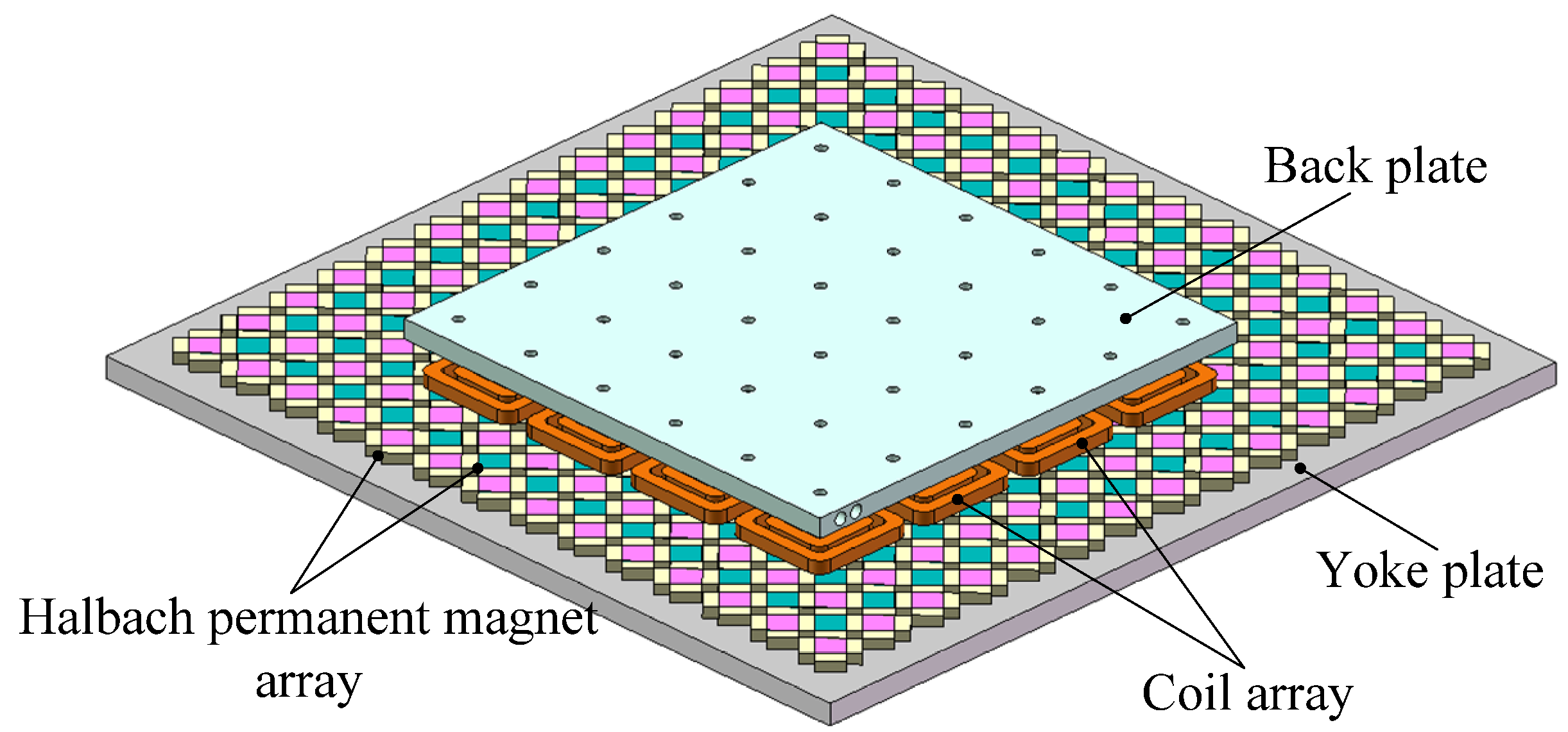
2.1. Basic Structure and Working Principle

Figure 1 shows the basic structure of the concentric maglev planar motor. It adopts the coreless moving-winding structure. The mover consists of the base plate and 16 sets of the concentric winding, which are displayed as 4 × 4. The stator consists of the yoke plate and the new-type Halbach permanent magnet array, which is rotated 45 degrees from the traditional Halbach [32] permanent magnet array.
The working principle of the proposed planar motor is described as follows. The permanent magnet generates a magnetic field, in which the windings with current in them will generate electromagnetic force and electromagnetic torque. There is no constraint on the motor mover, thus the mover can move in six degrees of freedom. To realize the full control of the movement in six degrees of freedom, all the windings on the mover need to be controlled properly. After the 16 windings are fixed to the mover, the position of the 16 windings relevant to the stator can be known by the relevant position between the mover and the stator. Thus, the relationship between the electromagnetic forces (and torques) and the respective current in the winding can be derived. Through the decoupling calculation, we can get the needed current in each winding for the expected forces and torques. Therefore, the multi-degree freedom of control of the proposed maglev planar motor can be realized.

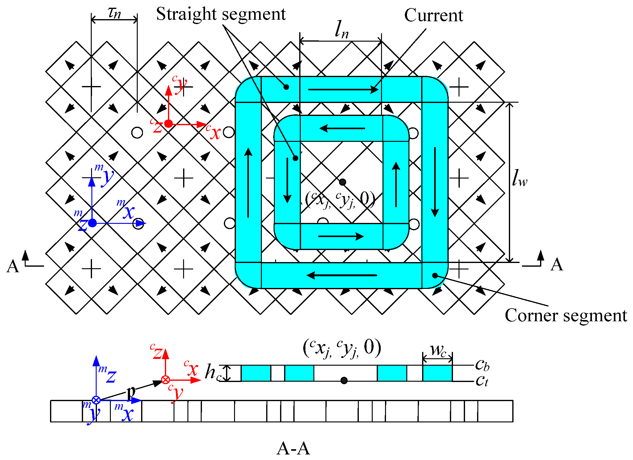
2.2. Winding Model and Parameter Definition

The whole concentric winding (see Figure 2) consists of the outer coil and the inner coil, which are connected in series. The directions of the currents in them are just the opposite. The whole winding is then divided into four long straight segments, four short straight segments, and eight corner segments. The electromagnetic force and torque can be derived by calculating separately. In Figure 2, τn denotes the pole pitch, lw denotes the outer winding length of the straight coil segment, ln denotes the inner coil length of the straight segment, hc is the thickness of the coil, wc is the width of the coil, ct and cb are the height coordinates of the coil.

2.3. Coordinate Definitions and Transformation

Three different coordinate systems are defined in Figure 2 and Figure 3. The first one is the stator global coordinate system denoted with the superscript m, which is fixed on the top face of the stator permanent magnet. It can be expressed as
x m = [ x m y m z m ] T
The second one is the mover local coordinate system denoted with the superscript c, which is fixed on the mover bottom surface center. It can be expressed as
x c = [ x c y c z c ] T
The third one is the corner local coordinate system denoted with the superscript s. It can be expressed as
x s = [ x s y s z s ] T
The vector p is the position vector of the mover local coordinate system in the global coordinate system. It can be expressed as
p = [ p x p y p z ] T
The coordinate position of the j-th winding center in the mover local coordinate system can be expressed as
x j c = [ x j c y j c z j c ] T
The two coordinate systems can be converted into each other with the coordinate transformation. For example, the vector in the mover local coordinate system and that in the global coordinate system can be transformed into each other through the following equations
x m = R c m x c + p
x c = R m c ( x m p )
The orientation transformation matrix is defined as
R c m = R o t ( x c , ψ ) R o t ( y c , θ ) R o t ( z c , ϕ )
R m c = R c 1 m = R c T m
where
R o t ( x c , ψ ) = [ 1 0 0 0 cos ( ψ ) sin ( ψ ) 0 sin ( ψ ) cos ( ψ ) ]
R o t ( y c , θ ) = [ cos ( θ ) 0 sin ( θ ) 0 1 0 sin ( θ ) 0 cos ( θ ) ]
R o t ( z c , ϕ ) = [ cos ( ϕ ) sin ( ϕ ) 0 sin ( ϕ ) cos ( ϕ ) 0 0 0 1 ]
and in the above equations ψ , θ , and ϕ are the rotation angles about the cx-, cy-, and cz-axes, respectively. Thus, the position and orientation of the translator can be described in six degrees of freedom.

3. Electromagnetic Force and Torque

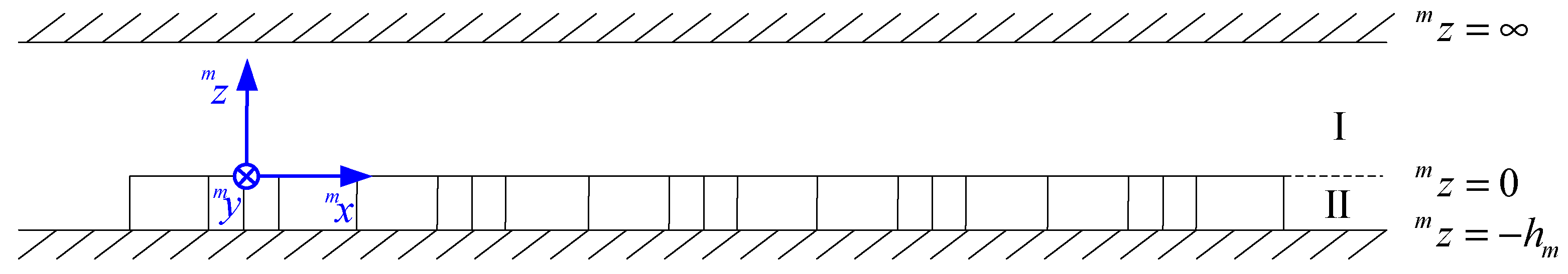
3.1. Permanent Magnet Array Model

To get the mathematic model of the electromagnetic force and torque, the gap magnetic field generated by the Halbach permanent magnet arrangement in Figure 2 needs to be calculated first. To simplify the analysis, the following assumptions are made:
  • The relative permeability of the iron yoke has a value of infinity;
  • The magnet array has a periodicity over the mx and my direction and the magnetization value of the permanent magnet is not changed;
  • Ending effect is neglected.
The analysis model of the Halbach magnet array, the three-dimensional space is divided into two regions, region I is in the air and the permanent magnets in region II are located in between −hmmz ≤ 0. For region II, the permeability μ = μ0μr, where μr is the relative permeability of the permanent magnets, μ0 is the permeability of free space.
A magnetic scalar potential φ is introduced in both charge free regions to solve the problem. The magnetic scalar potential in the air (regions I in Figure 3) is governed by Laplace’s equation and in the permanent magnets by Poisson’s equation [4,27].
The boundary conditions are as follows. The subscript I and II denote the air region and the magnets region respectively, and mx, my, mz mean the components of the three directions.
φ 1 ( x m , y m , + ) = 0
φ 2 ( x m , y m , h m ) = 0
H 1 x ( x m , y m , 0 ) = H 2 x ( x m , y m , 0 )
H 1 y ( x m , y m , 0 ) = H 2 y ( x m , y m , 0 )
B 1 z ( x m , y m , 0 ) = B 2 z ( x m , y m , 0 )
where hm is the thickness of the magnetization thickness of the permanent magnet, H is the magnetic field strength, B is the magnetic flux density.
Based on Maxwell electromagnetic field theory, the magnetic flux density is the sum of Fourier harmonic components. In general, only the first harmonic component is taken into account in the maglev planar motor force and torque real-time model to realize the fast calculation. When high harmonic components are neglected, the paper [28,33] states that the Halbach permanent magnet array magnetic flux density, with the counterclockwise rotation direction as the positive direction, can be transformed in the global coordinate system and expressed as
B m ( x m ) = e π τ n m z B x y m ( x m ) = e π τ n m z [ B x y 2 sin ( π τ n x m ) B x y 2 sin ( π τ n y m ) B z 2 ( cos ( π τ n y m ) cos ( π τ n x m ) ) ]
where Bxy and Bz are the amplitudes of the mean value of the magnetic flux density components in the cross section of the coil at mz = 0. Thus, it can be derived as
B z = 2 B x y
The above equation can be transformed into that in the local coordinate system of the mover
B c ( x c , p ) = R m c B m ( R c m ( x c + p ) )
The two coordinate systems only have relevant translation movement without rotation to each other. Thus, it can be derived as follows
R m c = R c 1 m = [ 1 0 0 0 1 0 0 0 1 ]
Furthermore, the magnetic flux density in the mover local coordinate system can be derived as
B c ( x c , p ) = e π τ n ( z c + p z ) B x y c ( x c , p ) = e π τ n ( z c + p z ) [ B x y 2 sin ( π τ n ( x c + p x ) ) B x y 2 sin ( π τ n ( y c + p y ) ) B z 2 ( cos ( π τ n ( y c + p y ) ) cos ( π τ n ( x c + p x ) ) ) ]

3.2. Force and Torque on Straight Segment

The goal of this paper is to derive a set of basic equations which predict the forces and torques produced in the actuator. Three simplifications are made to obtain this model:
  • The magnetic flux density distribution of the Halbach permanent magnet array is modeled by a 2-D sine wave;
  • The coils are replaced by filament ones;
  • The coil and magnet arrays are rigid.
The forces and torques are calculated with the Lorentz force method. According to the Lorenz’s law of force, the electromagnetic force and torque on the winding can be derived when the magnetic flux density and the current in the winding are known. The force on the mover is opposite to the force on the coils. The Lorentz force and torque equations are
F = V J × B d V
T = V r × ( J × B ) d V
where B is the magnetic flux density of the magnet array, J is the volume current density in the coil, V is the volume of the coil, r is the vector from the point about which the torque is calculated.
In the maglev planar motor with the concentric winding structure, the magnetic field generated by the Halbach permanent magnet is exponentially decayed in the vertical direction. In the mover local coordinate system, the electromagnetic force on the straight segment of the coil can be derived as
F l c = V J c × B c ( x c , p ) d V = C z J c × B x y c ( x c , p ) d x c d y c
where
C z = c t c b e π τ n z m d z m = c t c b e π τ n ( z c + p z ) d z c
As shown in Figure 2, the concentric winding coil consists of the inner coil and the outer coil. Thus, the force on the whole coil can be expressed as
F l c = F l o u t c + F l i n c
The methods to calculate the forces on the inner and outer coils are the same. Taking the outer coil as an example, the force can be calculated as
F l o u t j c = C z ( y j c + l w 2 y j c + l w 2 + w c x j c l w 2 x j c + l w 2 [ J 0 0 ] × B x y c ( x c , p ) d x c d y c + y j c l w 2 y j c + l w 2 x j c + l w 2 x j c + l w 2 + w c [ 0 J 0 ] × B x y c ( x c , p ) d x c d y c + y j c l w 2 w c y j c l w 2 x j c l w 2 x j c + l w 2 [ J 0 0 ] × B x y c ( x c , p ) d x c d y c + y j c l w 2 y j c + l w 2 x j c l w 2 w c x j c l w 2 [ 0 J 0 ] × B x y c ( x c , p ) d x c d y c )
where cxj and cyj are the coordinate positions for the j winding.
The same approach is applied to the torque. The volume integral to calculate the torque can also be split into an integral over cz and a surface integral over cx and cy, In the mover local coordinate system. The electromagnetic torque on the straight segment of the coil can be derived as
T l c = V r × ( J c × B c ( x c , p ) ) d V = C z [ x c y c r z c ] × ( J c × B x y c ( x c , p ) ) d x c d y c
where crz is the equivalent force arm in the cz-direction.
Similar to the analysis of the force, the torque on the winding can be expressed as
T l c = T l o u t c + T l i n c
Taking the outer coil as an example, the torque can be calculated as
T l o u t j c = C z ( y j c + l w 2 y j c + l w 2 + w c x j c l w 2 x j c + l w 2 [ x c y c r z c ] × ( [ J 0 0 ] × B x y c ( x c , p ) ) d x c d y c + y j c l w 2 y j c + l w 2 x j c + l w 2 x j c + l w 2 + w c [ x c y c r z c ] × ( [ 0 J 0 ] × B x y c ( x c , p ) ) d x c d y c + y j c l w 2 w c y j c l w 2 x j c l w 2 x j c + l w 2 [ x c y c r z c ] × ( [ J 0 0 ] × B x y c ( x c , p ) ) d x c d y c + y j c l w 2 y j c + l w 2 x j c l w 2 w c x j c l w 2 [ x c y c r z c ] × ( [ 0 J 0 ] × B x y c ( x c , p ) ) d x c d y c )
Based on Equations (27), (28), (30), and (31), the three forces cFxj, cFyj, cFzj and the three torques cTxj, cTyj, cTzj can be derived.

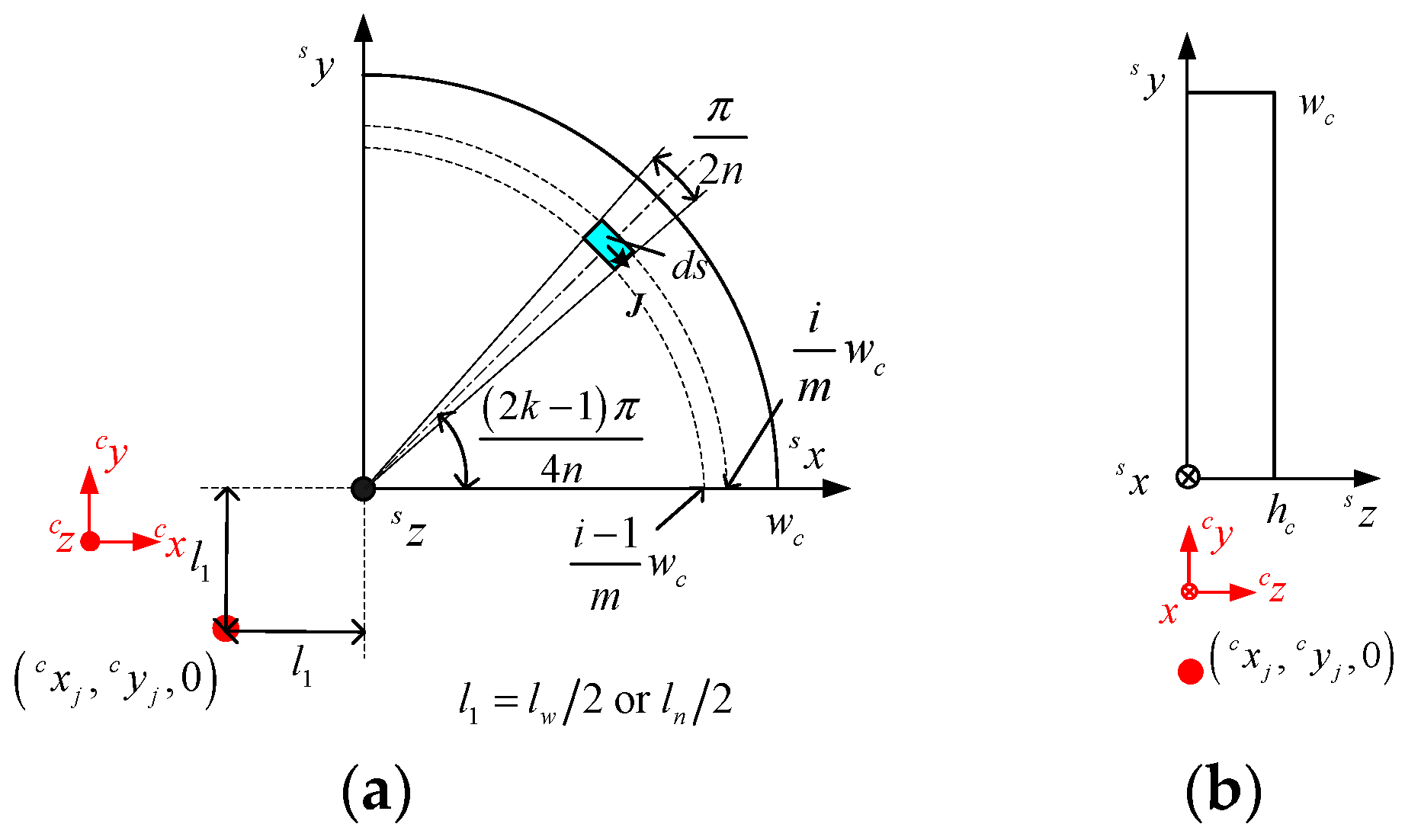
3.3. Force and Torque on Corner Segment

The computation model using only the straight segment of the coil does not take the corner segment into account. Thus, the accuracy of the computation model is not high, which is one of the major reasons for the fluctuation of the force and torque of the maglev planar motor. To reduce the fluctuation, the corner segment cannot be neglected. The force and torque on the corner segment can be derived through the numerical calculation method.
One coil has four corner segments. For different corner segments, the rotation matrix can be used according to the relation between the respective corner coordinate system and the mover coordinate system. In the subdivision area, the magnetic flux density value and direction can be seen as identical and the force and torque on the corner segment (see Figure 4) of the coil based on numerical calculation method can be expressed as
F c j 1 c = C z lim m , n + i = 1 m k = 1 n π w c 2 2 i 1 4 n m 2 J [ sin ( ( 2 k 1 ) π 4 n ) cos ( ( 2 k 1 ) π 4 n ) 0 ] × [ B x y 2 sin ( π τ n ( x s + l w 2 + x j c + p x ) ) B x y 2 sin ( π τ n ( y s + l w 2 + y j c + p y ) ) B z 2 ( cos ( π τ n ( y s + l w 2 + y j c + p y ) ) cos ( π τ n ( x s + l w 2 + x j c + p x ) ) ) ]
T c j 1 c = C z lim m , n + i = 1 m k = 1 n π w c 2 2 i 1 4 n m 2 [ x j c + x s + l w 2 y j c + y s + l w 2 r z c ] × ( J [ sin ( ( 2 k 1 ) π 4 n ) cos ( ( 2 k 1 ) π 4 n ) 0 ] × [ B x y 2 sin ( π τ n ( x s + l w 2 + x j c + p x ) ) B x y 2 sin ( π τ n ( y s + l w 2 + y j c + p y ) ) B z 2 ( cos ( π τ n ( y s + l w 2 + y j c + p y ) ) cos ( π τ n ( x s + l w 2 + x j c + p x ) ) ) ] )
where
x s = 2 i 1 2 m w c cos ( π ( 2 k 1 ) 4 n )
y s = 2 i 1 2 m w c sin ( π ( 2 k 1 ) 4 n )
Equations (32) and (33) present the method to calculate the electromagnetic force and torque for one corner. Likewise, the other force and torque for the other three corners can be derived.

3.4. Accurate Real-Time Equation of Electromagnetic Force and Torque

According to the calculation results of straight and corner segments, the electromagnetic force and torque on the concentric winding can be derived as
F x j c = C z J B z sin ( π τ n ( x j c + p x ) ) ( C 1 + C x )
F y j c = C z J B z sin ( π τ n ( y j c + p y ) ) ( C 1 + C y )
F z j c = 2 C z J B x y ( cos ( π τ n ( x j c + p x ) ) ( C 1 + C x ) cos ( π τ n ( y j c + p y ) ) ( C 1 + C y ) )
T x j c = y j c F z j c r z c F y j c + 2 C z J B x y sin ( π τ n ( y j c + p y ) ) ( C 2 + τ n π C 1 + C y 1 )
T y j c = r z c F x j c x j c F z j c + 2 C z J B x y sin ( π τ n ( x j c + p x ) ) ( C 2 + τ n π C 1 + C x 1 )
T z j c = F y j c x j c F x j c y j c
where
C 1 = τ n π ( l w ( cos ( π τ n ( l w 2 + w c ) ) cos ( π τ n l w 2 ) ) l n ( cos ( π τ n ( l n 2 + w c ) ) cos ( π τ n l n 2 ) ) )
C 2 = τ n π ( l w ( l w 2 + w c ) sin ( π τ n ( l w 2 + w c ) ) ( l w 2 2 ) sin ( π τ n l w 2 ) ) τ n π ( l n ( l n 2 + w c ) sin ( π τ n ( l n 2 + w c ) ) ( l n 2 2 ) sin ( π τ n l n 2 ) )
C x = π w c 2 lim m , n + i = 1 m k = 1 n 2 i 1 n m 2 cos ( π ( 2 k 1 ) 4 n ) cos ( π τ n ( x s + l w + l n 4 ) ) sin ( π ( l n l w ) 4 τ n )
C y = π w c 2 lim m , n + i = 1 m k = 1 n 2 i 1 n m 2 sin ( π ( 2 k 1 ) 4 n ) cos ( π τ n ( y s + l w + l n 4 ) ) sin ( π ( l n l w ) 4 τ n )
C x 1 = π w c 2 lim m , n + i = 1 m k = 1 n 2 i 1 2 n m 2 cos ( ( 2 k 1 ) π 4 n ) × ( cos ( π τ n ( x s + l n 2 ) ) ( x s + l n 2 ) cos ( π τ n ( x s + l w 2 ) ) ( x s + l w 2 ) )
C y 1 = π w c 2 lim m , n + i = 1 m k = 1 n 2 i 1 2 n m 2 sin ( ( 2 k 1 ) π 4 n ) × ( cos ( π τ n ( y s + l n 2 ) ) ( y s + l n 2 ) cos ( π τ n ( y s + l w 2 ) ) ( y s + l w 2 ) )
The electromagnetic model of the whole winding can be derived when the equations for both the straight and corner segment are added together. Once the permanent magnet array and winding size are determined, the numerical value of C1, C2, Cx, Cy, Cx1, and Cy1 can be derived. Once the winding is put on the mover, the position deviation on the cx-cy plane can be seen as a constant, therefore, the whole electromagnetic force and torque on the mover is the sum result of that on each winding, taking the position deviation into account.

4. Validation and Analysis

The electromagnetic model is made of 16 sets of coils. After the 16 sets are fixed on the mover, the position cxj and cyj of each winding can be known. The electromagnetic force and torque on each winding is different due to the phase difference among them. They, however, share the same pattern depending on the position. It can be seen from Equations (36)–(41) that different windings have different cxj and cyj due to the different relevant position to the magnetic field, and the relevant position is the real factor that affects the force on each coil. The calculation results of this electromagnetic model can be validated by using the harmonic model [34,35]. The electromagnetic model parameters are show in Table 1.

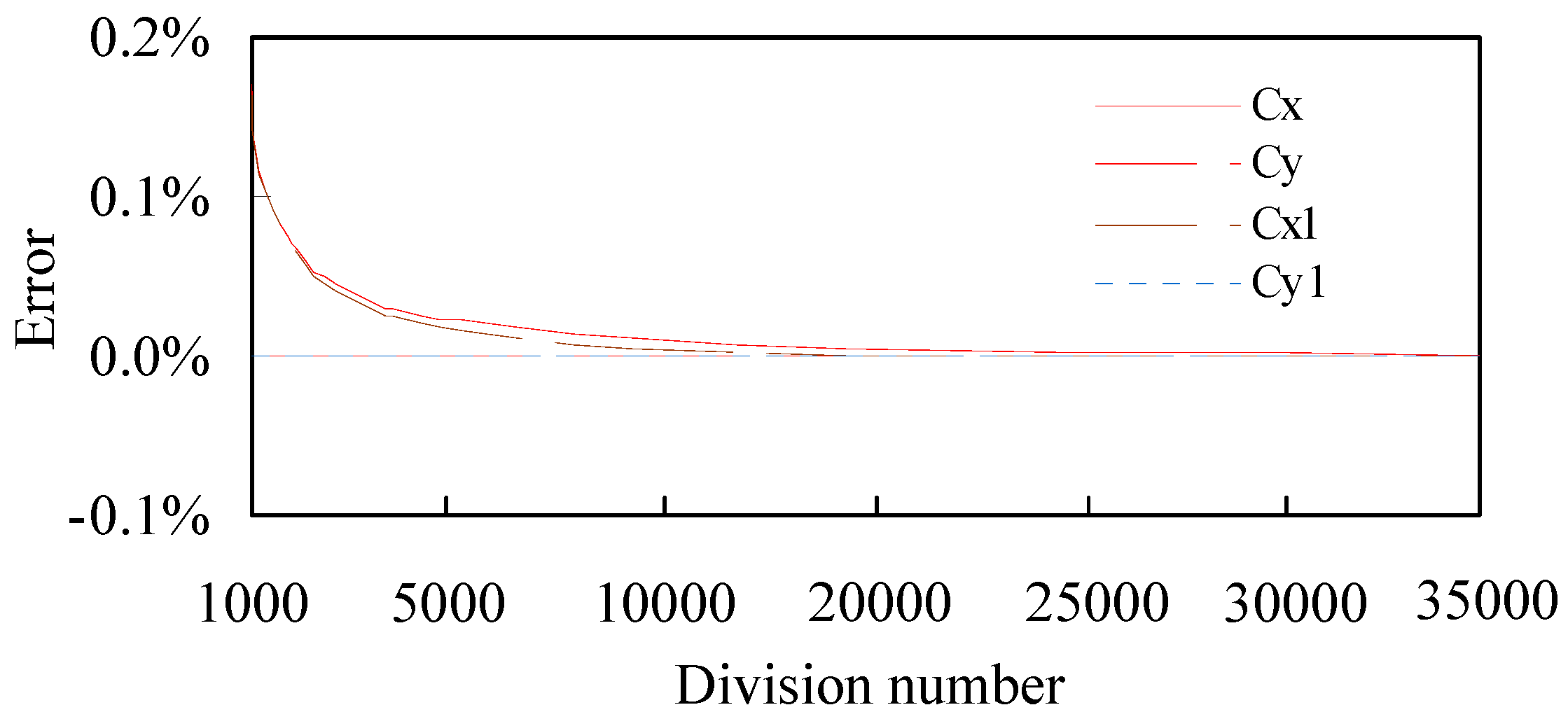
4.1. Precision Analysis of Coefficient

Equations (44)–(47) the accuracy of the numerical value Cx, Cy, Cx1, and Cy1 increases with the increase of the subdivision numbers. Figure 5 gives the relation between the four numerical solutions and the subdivision amount m and n. With five significant figures as the goal, when m ≥ 35,000 and n ≥ 35,000, all of the four coefficients can achieve this significance level; when m ≥ 5000 and n ≥ 5000, all the four coefficients can reach four significant figures.

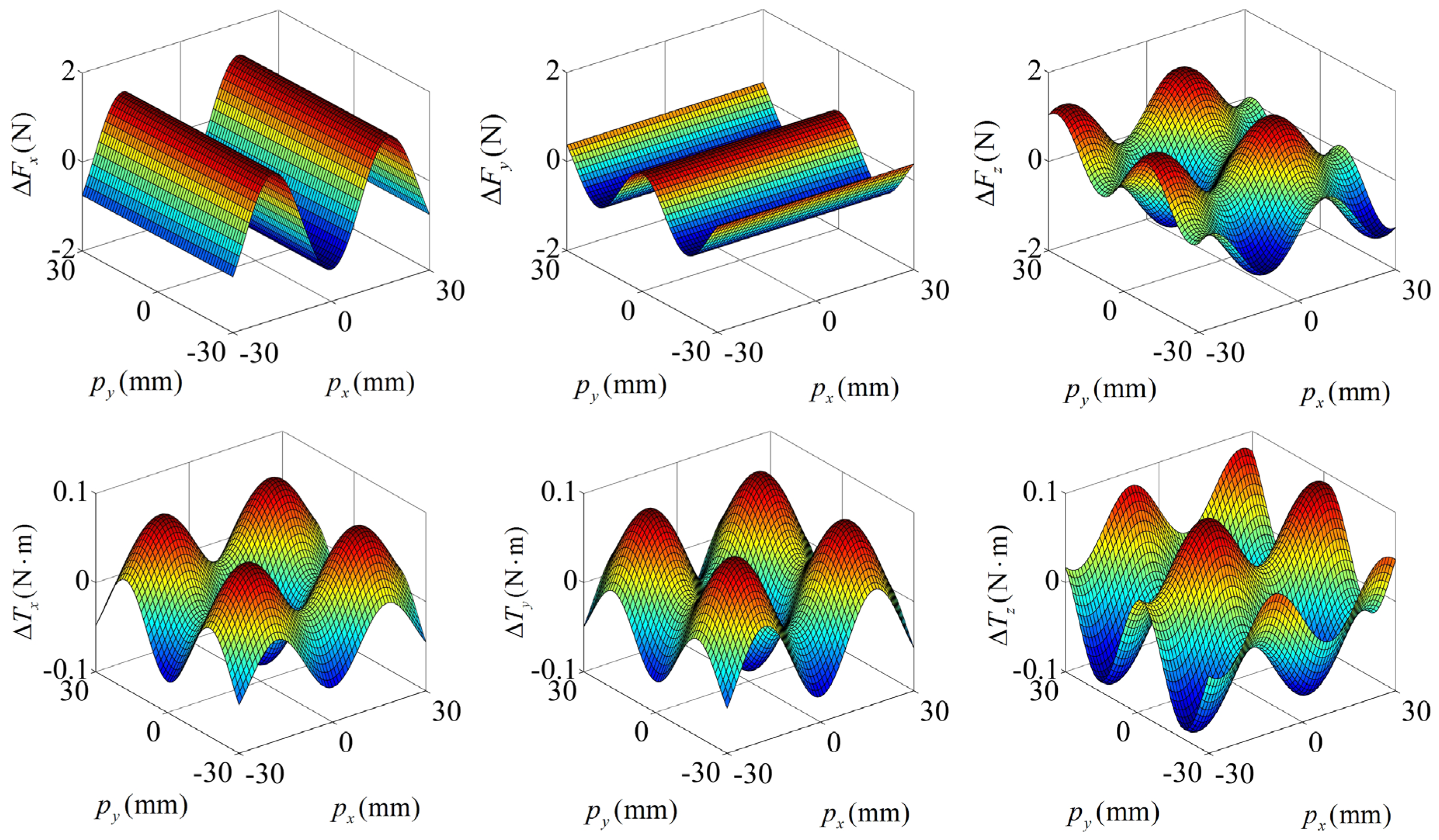
4.2. Precision Validation of Model

The computation model of maglev planar motor is verified by comparison with the harmonic model. In Figure 6, the displacement in the direction of px is from −30 mm to 30 mm, the same displacement length and the same sampling method are applied to the direction of py. The harmonic coefficient is set to be 1, to prevent the winding force and torque from neutralizing each other too much, the current of ±2 A is imposed on certain groups of windings.
The peak values calculated by the harmonic model are 91.93 N for Fx, 45.93 N for Fy, 91.97 N for Fz, 5.75 N·m for Tx, 6.21 N·m for Ty, and 6.82 N·m for Tz. It can be seen from Figure 6 that the error of the deduced model of maglev planar motor in this paper is minor, the maximum of the error is 1.41% for the force and torque. Compared with the well-known harmonic model, the proposed model has high accuracy and can realize practical application easily as well.

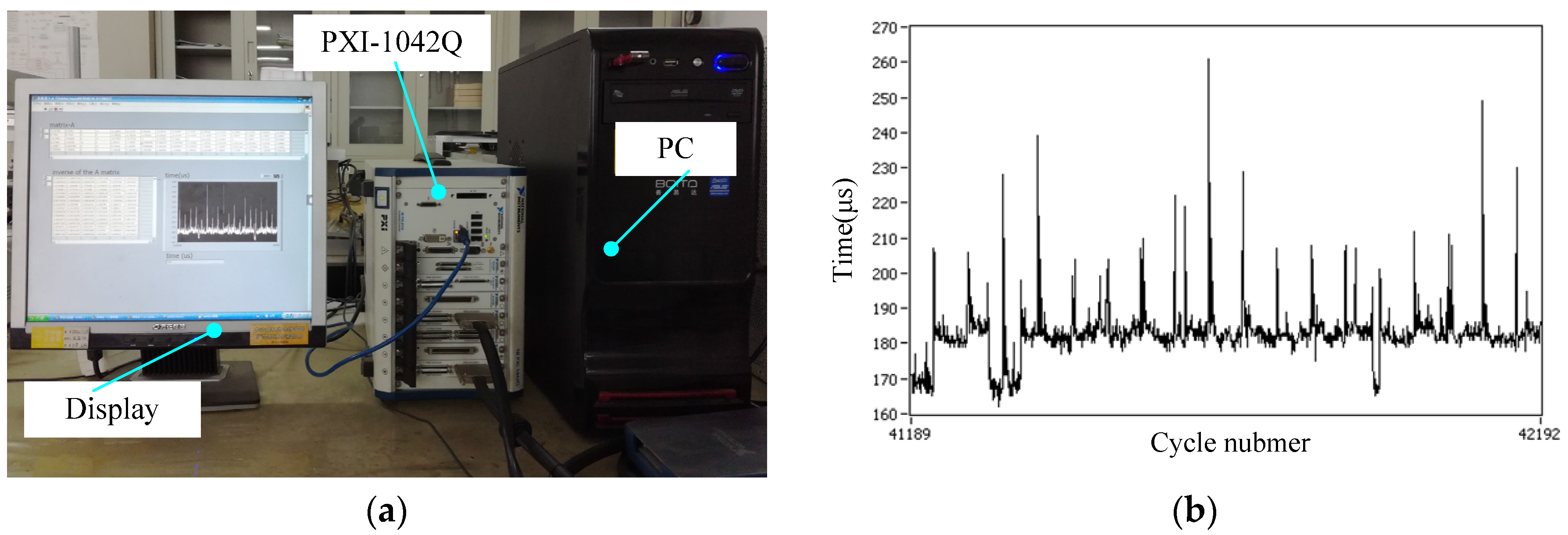
4.3. Real-Time Ability Validation of Model

The proposed computation model seems to be more complex than the other models [27,28] in terms of the mathematical expression. Nevertheless, the coefficient on that mathematical expression can be expressed a constant after all the motor structure sizes are fixed. Thus, the computation speed of it in the practical application is the same as that of the conventional electromagnetic model. Only the coefficient in the mathematical expression is more close to the real value, which guarantees the accuracy of the proposed model. Thus, it can be concluded fairly that the proposed model has higher accuracy but without adding additional computation complexity in the control process, which makes it suitable for high-accuracy real-time practical application. Using NI PXI-1042Q to validate the program, the result is shown in Figure 7a with the PXI-1042Q operating in a real-time system to validate the proposed electromagnetic model and the computation speed of solving the generalized inverse matrix. Figure 7b shows the measured results of the running time for each loop. It can be seen that the average running time is 183 μm and the maximum is 264 μm, which can meet the control requirement of the maglev planar motor.

5. Conclusions

This paper proposes a new accurate real-time computation model of the electromagnetic force and torque for the concentric winding used in a maglev planar motor. The proposed computation model does not simplify the corner segment, which means it has more accuracy regarding the real physical situation. Compared with the traditional method, the new model has an extra corner coefficient. After the motor structure is fixed, however, the corner segment and straight segment coefficients can be added together and thus it has the same computation time as that of the traditional model. The harmonic model is used to validate the proposed computation model and the NI-PXI 1042Q platform is used to validate the real-time ability of the motor model and the decoupling computation. The validation result shows that the proposed real-time computation model is found to have smaller model error. Thus, it can be concluded that the proposed new accurate real-time computation model can be used in the real-time decoupling current computation for better control accuracy in the maglev planar control system.

Acknowledgments

This work was supported in part by the National Science and Technology Major Project (2009ZX02207-001), in part by the China Postdoctoral Science Foundation Funded Project (2015M80262), in part by the State Key Program of National Natural Science of China under Grant (51537002), the National Natural Science Foundation of China (51607044), and in part by “the Fundamental Research Funds for the Central Universities” (Grant No. HIT. NSRIF. 2017010).

Author Contributions

Design of the research scheme and research supervision: Baoquan Kou, Feng Xing, and Lu Zhang. Performing of the research and writing of the manuscript: Chaoning Zhang and Yiheng Zhou.

Conflicts of Interest

The authors declare no conflict of interest.

References

  1. Rovers, J.M.M.; Jansen, J.W.; Compter, J.C.; Lomonova, E.A. Analysis Method of the Dynamic Force and Torque Distribution in the Magnet Array of a Commutated Magnetically Levitated Planar Actuator. IEEE Trans. Magn. 2012, 59, 2157–2166. [Google Scholar] [CrossRef]
  2. Nguyen, V.H.; Kim, J.W. Design and control of a compact lightweight planar position moving over a concentrated-Field Magnet Matrix. IEEE Trans. Mech. 2013, 18, 1090–1099. [Google Scholar] [CrossRef]
  3. Jansen, J.W.; Lomonova, E.A.; Vandenput, A.J.A.; Van Lierop, C.M.M. Analytical Model of a Magnetically Levitated Linear Actuator. In Proceedings of the IEEE Industry Applications Conference fourtieth IAS Annual Meeting, Hong Kong, China, 2–6 October 2005; pp. 2107–2113.
  4. Jansen, J.W.; Van Lierop, C.M.M.; Lomonova, E.A. Magnetically levitated planar actuator with moving magnets. IEEE Trans. Ind. Appl. 2008, 44, 1108–1115. [Google Scholar] [CrossRef]
  5. Ueda, Y.; Ohsaki, H. A planar actuator with a small mover traveling over large Yaw and translational displacements. IEEE Trans. Magn. 2008, 44, 609–616. [Google Scholar] [CrossRef]
  6. Christian, S.-R.J.; Kim, W.J. Multivariable control and optimization of a compact 6-DOF precision positioner with hybrid H-2/H-infinity and digital filtering. IEEE Trans. Control Syst. Technol. 2013, 21, 1641–1651. [Google Scholar]
  7. Cao, J.Y.; Zhu, Y.; Wang, J.S.; Yin, W.S.; Duan, G.H. A Novel Synchronous Permanent Magnet Planar Motor and Its Model for Control Applications. IEEE Trans. Magn. 2005, 41, 2156–2163. [Google Scholar]
  8. Choi, J.H.; Park, J.H.; Baek, Y.S. Design and Experimental Validation of Performance for a Maglev Moving-Magnet-Type Synchronous PM Planar Moto. IEEE Trans. Magn. 2006, 42, 3419–3421. [Google Scholar] [CrossRef]
  9. De Boeij, J.; Lomonova, J.E.; Vandenput, A. Modeling ironless permanent-magnet planar actuator structures. IEEE Trans. Magn. 2006, 42, 2009–2016. [Google Scholar] [CrossRef]
  10. Daiki, E.; Masaya, W. Study of a basic structure of surface actuator. IEEE Trans. Magn. 1989, 25, 3916–3918. [Google Scholar]
  11. Kook, R.S.; Park, J.K. A Compact Ultra-precision Air Bearing Stage with 3-DOF Planar Motions Using Electromagnetic Motors. Int. J. Precis. Eng. Manuf. 2011, 12, 115–119. [Google Scholar]
  12. Compter, J.C. Electro-dynamic planar motor. J. Precis. Eng. 2004, 28, 171–180. [Google Scholar] [CrossRef]
  13. Rovers, J.M.M.; Jansen, J.W.; Lomonova, E.A. Multiphysical analysis of moving-magnet planar motor topologies. IEEE Trans. Magn. 2013, 49, 5730–5741. [Google Scholar] [CrossRef]
  14. Vandenput, A.J.A.; Lomonova, E.A.; Makarovic, J.; Hol, S.A.J.; Lebedev, A.; Jansen, J.W. Novel types of the multi-degrees-of-freedom electro-magnetic actuators. In Proceedings of the International Symposium on Power Electronics, Electrical Drives, Automation and Motion, Taormina, Italy, 23–26 May 2006; pp. 1056–1062.
  15. Compter, J.C.; Jansen, J.W.; Lomonova, E.A.; Vandenput, A.J.A. Six degrees of freedom planar motors. In Proceedings of the 4th Euspen International Conference, Glasgow, UK, 31 May—2 June 2004; pp. 390–391.
  16. Van Lierop, C.M.M.; Jansen, J.W.; Lomonova, E.A.; Damen, A.A.H.; Van den Bosch, P.P.J.; Vandenput, A.J.A. Commutation of a magnetically levitated planar actuator with moving-magnets. IEEE Trans. Ind. Appl. 2008, 128, 1333–1338. [Google Scholar] [CrossRef]
  17. Min, W.; Zhang, M.; Zhu, Y.; Chen, B.D.; Duan, G.H.; Hu, J.C.; Yin, W.S. Analysis and optimization of a new 2-D magnet array for planar motor. IEEE Trans. Magn. 2010, 46, 1167–1171. [Google Scholar] [CrossRef]
  18. Zhang, L.; Kou, B.Q.; Zhang, H.; Guo, S.L. Characteristic Analysis of a Long-Stroke Synchronous Permanent Magnet Planar Motor. IEEE Trans. Magn. 2012, 48, 4658–4661. [Google Scholar] [CrossRef]
  19. Jansen, J.W.; Smeets, J.P.C.; Overboom, T.T.; Rovers, J.M.M.; Lomonova, E.A. Overview of Analytical Models for the Design of Linear and Planar Motors. IEEE Trans. Magn. 2014, 50, 39–52. [Google Scholar] [CrossRef]
  20. Rovers, J.M.M.; Jansen, J.W.; Lomonova, E.A. Force and Torque Errors Due to Manufacturing Tolerances in Planar Actuators. IEEE Trans. Magn. 2012, 48, 3116–3119. [Google Scholar] [CrossRef]
  21. Zhang, L.; Kou, B.Q.; Li, L.Y. Modeling and Design of an Integrated Winding Synchronous Permanent Magnet Planar Motor. IEEE Trans. Plasma Sci. 2013, 41, 1214–1219. [Google Scholar] [CrossRef]
  22. Rovers, J.M.M.; Jansen, J.W.; Lomonova, E.A. Analytical calculation of the force between a rectangular coil and a cuboidal permanent magnet. IEEE Trans. Magn. 2010, 46, 1656–1659. [Google Scholar] [CrossRef]
  23. Hamers, H.R. Actuation Principles of Permanent Magnet Synchronous Planar Motors: A Literature Survey; Working Paper; Eindhoven University of Technology: Eindhoven, The Netherlands, 2005. [Google Scholar]
  24. Van Lierop, C.M.M.; Jansen, J.W.; Damen, A.A.H.; Lomonova, E.A.; Van den Bosch, P.P.J.; Vandenput, A.J.A. Model-Based Commutation of a Long-Stroke Magnetically Levitated Linear Actuator. IEEE Trans. Ind. Appl. 2009, 45, 1982–1990. [Google Scholar] [CrossRef]
  25. Achtenberg, J.; Rovers, J.M.M.; Van Lierop, C.M.M.; Jansen, J.W.; Van den Bosch, P.P.J.; Lomonova, E.A. Model based commutation containing edge coils for a moving magnet planar actuator. IEEE Trans. Ind. Appl. 2010, 130, 1147–1152. [Google Scholar] [CrossRef]
  26. Kou, B.Q.; Zhang, H.; Li, L.Y. Analysis and Design of a Novel 3-DOF Lorentz-Force-Driven DC Planar Motor. IEEE Trans. Magn. 2011, 47, 2118–2126. [Google Scholar]
  27. Jansen, J.W.; Van Lierop, C.M.M.; Lomonova, E.A.; Vandenput, A.J.A. Modeling of magnetically levitated planar actuators with moving magnets. IEEE Trans. Magn. 2007, 43, 15–25. [Google Scholar] [CrossRef]
  28. Min, W.; Zhang, M.; Zhu, Y.; Liu, F.; Duan, G.; Hu, J.; Yin, W. Analysisand design of novel overlapping ironless windings for planar motors. IEEE Trans. Magn. 2011, 47, 4635–4642. [Google Scholar] [CrossRef]
  29. Verma, S.; Shakir, H.; Kim, W.J. Novel electromagnetic actuation scheme for multiaxis nanopositioning. IEEE Trans. Magn. 2006, 42, 2052–2062. [Google Scholar] [CrossRef]
  30. Zhu, H.Y.; Teo, T.J.; Pang, C.K. Design and Modeling of a Six Degrees-of-Freedom Magnetically Levitated Positioner Using Square Coils and 1D Halbach Arrays. IEEE Trans. Ind. Electron. 2016, 64, 440–450. [Google Scholar] [CrossRef]
  31. Xu, F.Q.; Dinavahi, V.; Xu, X. Parallel Computation of Wrench Model for Commutated Magnetically Levitated Planar Actuator. IEEE Trans. Ind. Electron. 2016, 63, 7621–7631. [Google Scholar] [CrossRef]
  32. Huang, R.; Feng, J. Magnetic Field Analysis of Permanent Magnet Array for Planar Motor Based on Equivalent Magnetic Charge Method. In Proceedings of the 10th World Congress on Intelligent Control and Automation, Beijing, China, 6–8 July 2012; pp. 3966–3970.
  33. Zhang, L.; Kou, B.Q.; Xing, F.; Luo, J. Modeling and Analysis of a Magnetically Levitated Synchronous Permanent Magnet Planar Motor with Concentric Structure Winding. In Proceedings of the Electromagnetic Launch Technology, La Jolla, CA, USA, 7–11 July 2014; pp. 1–6.
  34. Peng, J.; Zhou, Y.F.; Liu, G.D. Calculation of a New Real-Time Control Model for the Magnetically Levitated Ironless Planar Motor. IEEE Trans. Magn. 2013, 49, 1416–1422. [Google Scholar] [CrossRef]
  35. Jansen, J.W. Magnetically Levitated Planar Actuator with Moving Magnets: Electromechanical Analysis and Design. Ph.D. Thesis, Eindhoven University of Technology, Eindhoven, The Netherlands, November 2007. [Google Scholar]
Figure 1. Maglev planar motor structure.
Applsci 07 00098 g001
Figure 2. Top views and A-A view of the components of a maglev planar motor: a Halbach array and a concentric structure winding.
Applsci 07 00098 g002
Figure 3. Analysis model of the Halbach magnet array.
Applsci 07 00098 g003
Figure 4. Corner segment model. (a) Top view of the division of the corner segment; (b) Left view of the division of the corner segment. The corner segment is divided into n fan-shaped sectors and m sectors in the direction of the axis of sx.
Applsci 07 00098 g004
Figure 5. The relation between the four-numerical solution Cx, Cy, Cx1, and Cy1 and the subdivision amount m and n. For the corner segment of the coil, the angle is divided into 35,000 parts, the radius is divided into 35,000 parts, and m is equal to n.
Applsci 07 00098 g005
Figure 6. The force and torque errors between the deduced model and the harmonic model.
Applsci 07 00098 g006
Figure 7. Program running time analysis. (a) Real-time control platform based on NI PXI-1042Q; (b) Results of the program running time.
Applsci 07 00098 g007
Table 1. Electromagnetic model parameters.
ParameterValueUnit
Pole pitch τn17.7mm
Winding width wc11.8mm
Permanent magnet thickness hm20mm
Air gap h1mm
Winding thickness hc10mm
Outer coil straight segment length lw76.7mm
Inner coil straight segment length ln41.3mm
Magnetic flux density vertical component Bz0.81T
Number of turns Nc218-

