Heuristic Method for Decision-Making in Common Scheduling Problems

Abstract

The aim of the paper is to present a heuristic method for decision-making regarding an NP-hard scheduling problem with limitations related to tasks and the resources dependent on the current state of the process. The presented approach is based on the algebraic-logical meta-model (ALMM), which enables making collective decisions in successive process stages, not separately for individual objects or executors. Moreover, taking into account the limitations of the problem, it involves constructing only an acceptable solution and significantly reduces the amount of calculations. A general algorithm based on the presented method is composed of the following elements: preliminary analysis of the problem, techniques for the choice of decision at a given state, the pruning non-perspective trajectory, selection technique of the initial state for the trajectory final part, and the trajectory generation parameters modification. The paper includes applications of the presented approach to scheduling problems on unrelated parallel machines with a deadline and machine setup time dependent on the process state, where the relationship between tasks is defined by the graph. The article also presents the results of computational experiments.

1. Introduction

Scheduling problems are very widely presented and studied in the literature [1,2]. There are many different solutions for known problems (travelling salesman problem TSP [3], basic and different versions of Vehicle routing problem VRP) [4,5,6,7,8]. Moreover, there are also areas related to the specific features of scheduling problems. For example, the following classes of problems are considered: arc routing problems [9,10], time-dependent scheduling [11], stochastic scheduling problems [12,13], or production scheduling under uncertainty [14,15].

There are many different approaches used to solve scheduling problems, mathematical methods (e.g., Petri net, branch and bound, integer programming, constraint programming) [16,17,18], and heuristic methods (genetic algorithms, Tabu search, simulated annealing, and swarm intelligence method) [19,20,21,22]. The methods based on the discrete event system approach are also an important part of the solution [23]. Furthermore, the adaptation of cellular automata to solve scheduling problems is becoming more and more popular [24,25,26].

However, invention of new ways to work in real factories (new complex production lines, automation of production) or applying a holistic approach, rather than ones individual to executors and other resources, creates the need for new solutions and the development of existing methods.

The purpose of this paper is to present a heuristic method for a common decision-making problem, where there are limitations related to the task and the resources needed to perform the tasks are not fixed and dependent on the current state of the process. These problems may be related to the decision-making process, where the decision is not determined separately for one particular executor but commonly for several executors (people, machines) and the decision-making process is carried out in stages (we deal with a multi-stage decision-making process). In addition, not all decisions are possible at every stage due to the existing constraints. These problems are related to physical goods (processes of physical transformation of materials during technological operations, carried out by machines and resources) as well as intangible goods (processes related to products resulting from a human thought). The class of problems under consideration belongs to the class of NP-hard problems or even strongly NP-hard, and because of the computation time it is not effective to use the exact algorithms for such problems, especially the problems of a larger size. For this reason, algorithms for approximation solutions are usually proposed rather than an optimal solution.

Due to the specific properties of solving such problems (not all decisions can be taken in each moment), it is not possible to simply use the improvement algorithms. They can be directly applied only when the solution type can be defined a priori (for example, it is a permutation, set, vector, etc.). Therefore, it is necessary to apply a constructive approach that significantly reduces the number of impossible solutions. The presented approach is based on that introduced by Dudek-Dyduch [27,28], for which the general paradigm is the algebraic-logical meta-model; it uses a state space, in particular a state graph. This approach is similar to the discrete event system.

The approach presented here is a development of a method based on the use of semimetrics (proposed and presented in [27,28,29,30,31]) and methods of constructing a single solution (single trajectory) [32,33]. It is related to constructing the state graph by the final part of the trajectory generation—although not the whole graph but only its most perspective parts [34]. This paper constitutes a summary and extension of previous work and represents a generalized method that can be applied to a wide class of scheduling problems. The presented research is also part of a team effort to build an ALMM solver—an IT tool to optimize discrete processes that involve complex dependencies or constraints [35,36,37,38,39,40].

The paper is organized as follows. In Section 2 a mentioned class of problems is characterized. Section 3 includes an ALMM approach to multistage decision process and a definition of a multistage decision process (MDP) is presented. The solution graph searching based on ALMM is described in Section 4. Section 5 includes characteristics of the algorithm class that uses the ALMM approach and generates the final parts of trajectory. Section 6 focuses on the application of the presented approach to scheduling problems on unrelated parallel machines with a deadline and machine setup time, dependent on the process state where the relationship between tasks is defined by the graph. Section 7 contains the results of computational experiments. The last section contains conclusions and future work.

2. Class of the Scheduling Problem

In this article we consider common decision-making problems, where the ability to start a task depends on the state of the other tasks, and the resources needed to perform these tasks are not fixed but depend on the state of the process. An example is a project implementation by a performer’s team (e.g., programmers or building brigades). A real project is often not a simple execution of several operations but is composed of a number of tasks (jobs) that depend on each other. They have to be performed by various executors (understood as people or teams as well as machines). Although performers’ skills may be the same, their performance may vary when carrying out the same task. Thus, the execution time of particular tasks most frequently depends on the assigned executor. Typically task consists of a single operation and is performed by one executor (an individual or a group). However, executors should aim to achieving a common target, which is the realization of a project at minimal cost or minimal time, and meet the restrictions. Most often the restrictions refer to execution time, costs, and ordering of particular tasks. Very often milestones are fixed. This means that a deadline is determined for certain tasks, such as completing a certain project stage. In many projects tasks are dependent and the decision to start a task can only be made when another task is completed. Moreover, because the completed tasks may become resources for the realization of other tasks, some of the already realized tasks may facilitate or accelerate another task realization. An example is the implementation of an integration procedure during software development or putting stairs up in a raised building. In addition, the start of a task may involve the use of a previously completed task that has become a resource (e.g., it takes time to get to the abovementioned new stairs).

Thus, the described problems can also be treated as scheduling problems with time limits and increasing resources that depend on the project state (tasks that have been finished) and the aim of the project can be formulated as the determination of the order of such tasks and their assignment to particular executors, which would minimize the total project cost and meet the restrictions.

In the literature, various unrelated parallel machine scheduling problems are discussed. For example, an unrelated parallel machine scheduling problem with sequence-dependent setup times (UPMSP-SDST) is considered and a hybrid estimation of distribution algorithm with iterated greedy search (EDA-IG) is proposed for solving it [41]. However, this problem differs from the one described above because the objective is to minimize the maximum completion time of all jobs, all the jobs and machines are available at the initial time, and a setup time is job-sequence-dependent and machine-dependent (but not state-dependent).

In [42] the authors propose to solve the unrelated parallel machine scheduling problem under a Time-of-Use pricing scheme using a mixed integer linear programming (MILP) model and a column generation heuristic. However, the jobs are independent and available for processing at time 0.

Section 6 presents the problem that belongs to the described class, i.e., the project of constructing a network of headings by two different groups of executors.

3. ALMM Methodology

The use of exact algorithms to solve problems described in Section 2 is ineffective. Also, the direct application of iterative improvement algorithms (e.g., Simulated Annealing, Genetic Algorithms, Tabu Search) is difficult or impossible. The methods based on the algebraic-logical meta-model paradigm of multistage decision process (introduced by Dudek-Dyduch [27,28,29]) can be successfully applied to solve the abovementioned class of problems with their relationships and limitations. A description and development of the methodology are presented in detail in [30].

In ALMM methodology values of particular model elements do not have to be numerical. Therefore, the state and/or decision can be represented by names of elements (symbols) as well as some objects, for example, a finite set and sequence. Moreover, a set of possible decisions U_p, a set of non-admissible generalized states S_N, and a set of goal-generalized states S_G are formally defined with the use of a logical formula. This is the advantage of ALMM: it allows us to represent all kinds of information regarding the problem (including various temporal relationships and restrictions of the process) in a convenient way. Moreover, such an approach enables making collective decisions in successive process stages, not only for individual objects. The ALMM approach also allows discrete optimization of problems by finding optimal or suboptimal solutions. Using the ALMM approach allows for the reconstruction of the decision-making process as well as monitoring and tracking decisions.

Let us recall the definition of the algebraic-logical meta-model of a multistage decision-making process for a better understanding of the approach [27,28,30].

Definition 1 (ALMM of MDP).

Algebraic-logical model of multistage decision process (MDP) is defined by the sextuple:

$$MDP=\left(U,S,s_0,f,S_N,S_G\right),$$

(1)

where:

• U is a set of decisions,
• $S=X\times T$ is a set named a set of generalized states, X is a set of proper states, $T\subset {\mathcal{R}}^{+}\cup \left\{0\right\}$ is a subset of non-negative real numbers representing the time instants,
• $s_0=\left(x_0,t_0\right)$ is an initial generalized state,
• $f:U\times S\to S$ is a partial function called a transition function, (it does not have to be determined for all elements of the set $U\times S$),
• $S_N\subset S$ is a set of not admissible generalized states
• $S_G\subset S$ is, a set of goal generalized states, i.e., the states in which we want the process to take place at the end.

The transition function is defined by two functions, $f=\left(f_x,f_t\right)$ where $f_x:U\times X\times T\to X$ determines the next state, $f_t:U\times X\times T\to T$ determines the next time instant. It is assumed that the difference $∆t=f_t\left(u,x,t\right)-t$ has a value that is both finite and positive.

The following features are very important:

• all limitations concerning the decisions in a given state s can be defined in a convenient way by so-called sets of possible decisions $U_p\left(s\right)$, and defined as: $U_p\left(s\right)=\left\{u\in U:\left(u,s\right)\in Dom f\right\}$.
• sets U and X in the most general case may be presented as a Cartesian product $U=U^1\times U^2\times \cdots \times U^m$, $X=X^1\times X^2\times \cdots \times X^n$ i.e., $u=\left(u^1,u^2,\cdots ,u^m\right)$, $x=\left(x^1,x^2,\cdots ,x^n\right)$.
• the state and/or decision does not have to be numerical and can be represented by names of elements (symbols) as well as some objects, for example, a finite set and sequence.
• a particular decision $u^i$ represents separate decisions that may be taken at the same time and relate to a particular executor (resource).
• the sets $S_N$, $S_G$ and $U_p\left(s\right)$ are formally defined with the use of logical formulas.
• the decision sequence determines a trajectory. Only a trajectory that ends in the set of goal states $S_G$ is admissible.

4. Solution Graph Searching Based on ALMM

The approach presented in this paper uses the state space, in particular the state graph. It belongs to a group of solutions that designate a solution based on a multi-stage decision-making process and consists of generating a finite sequence trajectory. In particular, it can be used for problems where the quality criterion is additively separable and monotonically growing along the trajectory. The task of searching for a solution based on an algebraic-logical meta-model methodology is to find a sequence of decisions that define the admissible trajectory. On the other hand, the task of the process control optimization is to find such a sequence of admissible decisions for which the quality is the best. The trajectory is equivalent to finding the path in the generalized state space that joins the initial state $s_0=\left(x_0,t_0\right)$ with the state belonging to the finish set, that is, the set of goal states S_G or set of non-admissible states $S_N$. The notion of semimetrics in the state space, proposed by Dudek-Dyduch [27,28], is used to evaluate states and their belonging to characteristic states. Thus, the distances between the current state and the states of the characteristic sets (goal, non-admissible, or favorable) are determined during a single trajectory generation. Moreover, each trajectory, whether admissible or non-admissible, is analyzed and the knowledge gained is used to improve control while generating successive trajectories. Thus, knowledge of the control process is obtained from the analysis of the process description, each state of a single trajectory, and the results of a previously obtained solution (trajectory).

It should be noted that the generalized state graph has a structure similar to the tree structure. This is because even if for two generalized states $s_1=\left(x,t_1\right)$ and $s_2=\left(x,t_2\right)$ the proper state x is the same, then the generalized state will be different if there is even a very small time difference between $t_1$ and $t_2$.

Although the algebraic-logical model provides an examination of all solutions (because a set of possible decisions in each state can be determined), the approach described below facilitates constructing not the whole tree but only its most perspective part. The solution to the problem can be searched for in two ways. First, a successive trajectory can be generated independently, using information derived from the analysis of the obtained solutions to modify, for example, simulation parameters. The algorithm using that method of generating a single trajectory with the idea of learning was proposed in [28] and developed in [32,33]. Secondly, a new trajectory can be created by correcting the final part of previously generated trajectories [34]. It is important then to determine the rule for selecting this process state from which the new final part of the trajectory will be generated. This state is selected on the basis of the information obtained previously, in the form of specially chosen and calculated parameters in each state. A general method using a second way of finding a solution is the subject of this paper.

5. Characteristic of the Algorithm Class That Generates the Final Parts of the Trajectory

Algorithms of the class under consideration raise the possibility of improving the solution by constructing many acceptable solutions and choosing the best one. Generally an algorithm can generate all trajectories of the process and in this case the optimal solution can be found as long as an admissible solution exists. Taking into consideration the fact that the problems solved belong to the NP-hard class, the purpose is not to search the whole solution space but its most perspective part. The general form of the algorithm is as follows. Initially a preliminary analysis of the input data is performed. After verification that the existence of an admissible solution is not excluded, it is possible to start generating the trajectories. The first trajectory is generated from the initial state $s_0$. Each next state depends on the previous state and the decision made at that state, which is chosen from a set of possible decisions at the given state using a specific decision-making technique. Generation of the state sequence is terminated if the new state is a goal state, a non-admissible state, or a state with an empty set of possible decisions. It is possible to interrupt trajectory generating if only the quality criterion value for a given state is greater than the best quality criterion value of the found admissible trajectory. All states of constructed trajectories (first and subsequent) are stored together with the characteristic parameters. After construction of the first trajectory, the final parts of trajectory are subsequently generated, starting from one of the stored states chosen from a set of open states, using a specific selection technique. Thus, trajectories can also be constructed from the initial state. In this case, with a limited number of trajectories, it is extremely important to select the state from which the final part of trajectories is generated.

Concluding, the important features of the presented algorithm class are as follows:

• a trajectory sequence or a final part of the trajectory is generated, each trajectory is analyzed, and this analysis is used to obtain knowledge about the process and its control,
• all generated process states and their characteristic parameters (attributes) are stored,
• during the construction of the trajectory, the process state is analyzed and based on it the technique of selecting the decision in a given state can be modified,
• trajectory generating is interrupted if only the quality criterion value for a given state is greater than the best quality criterion value of the found admissible trajectory,
• the initial state of the final part of the trajectory is selected based on the analysis of characteristic parameters for stored states of trajectories that have been generated so far; if the selected state is the process initial state s₀ then the whole trajectory is generated,
• the results obtained so far can be used to make any modification related to the choice of general techniques and the initial state of the trajectory final part selection general techniques.

Therefore, distinctive components of the algorithm class that generate the final parts of the trajectory are as follow: the preliminary analysis of the problem, the technique of decision choice at a given state, the pruning non-perspective trajectory, selection technique of the initial state for the trajectory final part, and the trajectory generation parameters modification. An explanation of each component is below.

5.1. Preliminary Analysis of Problem

The input data analysis before starting the solutions search as well as gathering and information analysis is very important.

There are two main purposes of preliminary data analysis. The first one is verification of whether it is possible to exclude the existence of an admissible solution. There is no point in searching for this solution (the starting generation of any trajectory) when preliminary data analysis has determined that an admissible solution of the problem instance does not exist. Then trajectory generating is not started. However, the analysis does not always provide the correct information as to whether the admissible solution exists. Then trajectory generating is started, in spite of the fact that the admissible trajectory may not be determined at all.

The second aim of the initial data analysis of the problem (in particular the actual instances of the problem) is to define its characteristic features. The analysis can be performed in terms of belonging to a certain class of subproblems for which the best algorithm has been developed. In particular, it can help to set initial values of algorithm parameters and even the design of individual parts of the algorithm. Despite the fact that information obtained from the preliminary data analysis may be useful for further algorithm execution, this analysis could be very complicated. Thus, the cost and time of its use should not form a significant part of the cost and time of solutions determined by the algorithm.

5.2. Generating a Single Trajectory

The presented method consists of consecutive construction trajectories, starting from the initial state $s_0=\left(x_0,t_0\right)$ for whole trajectories or chosen state for the final part of the trajectory.

The trajectory generation process using the algebraic-logic model as follows. In each newly designated process state s a decision has to be chosen from a set of possible (sensible) decisions in the given state. Then, for the given state and chosen decision a new process state $s’=\left(x’,t’\right)$ is determined, with both the process of the proper state and the corresponding moment of time. They are calculated using the transition function of the process $f\left(x,t,u\right)$. If the new state belongs to the set of goal states $S_G$, the generation of the trajectory is completed successfully and its assessment can be made. If the new proper state or the corresponding moment of time does not meet the limitations, then this process state belongs to the set of non-admissible generalized states $S_N$. Then the trajectory generation is stopped (the trajectory is non-admissible). Figure 1 shows single trajectory constructing.

5.3. Decision Technique

Special attention will be paid here to the methods based on the ALMM methodology. One of the ways is to generate all the decisions from the set of possible decisions $U_p\left(s\right)$ that can be taken in a given state. These decisions are then evaluated and one of them is determined by local decision-making procedures. The literature presents a heuristic method of discrete optimization problems using local optimization, but in these methods local optimization was only based on minimization (maximization) of the local increase of quality criterion, whereas ALMM allows one to create sophisticated local optimization criteria, which takes into account much more information than just about the increase of the criterion. An example is a specially designed local optimization task, to determine the distance between a given state and a particular set of states (the states belonging to the set of non-admissible states $S_N$, as well as unfavorable states or distinguished favorable states), uses the term semimetrics (which differs from metrics in that it does not have to fulfill the condition $\psi \left(a,b\right)=0\iff a=b$). The idea of using a local criterion relating to additional limitation and semimetrics were first proposed by Dudek-Dyduch in [27] and developed in [26,29,32,34]. Then the decision with the smallest value of the local criterion is chosen. This local optimization criterion consists of three parts. The first part concerns the value of the global index of quality for the generated trajectory. It is a sum of the increase of the quality index resulting from the realization of the decision under consideration and the value related to the estimation of the quality index for the final trajectory section, which follows the possible realization of the decision under consideration. This part of the criterion is suitable for problems, for which the quality criterion is additively separable and monotonically ascending along the trajectory [27]. The components related to additional limitations or requirements are the second part of the criterion. The third part includes components responsible for the preference for certain types of decisions resulting from problem analysis. It should be emphasized that during the design of the criterion, the components of the second and third parts will also be closely related to the objective of optimization. Other components will be when the goal is to minimize project time (cost) or minimize the number of delayed tasks. Moreover, the coefficient (weight) is associated with each component. The higher the value of the coefficient, the greater the importance of the component. The knowledge gathered during constructing a trajectory is used to change these coefficients.

Another way to determine the decision in a given process state is using specially constructed rules. In this case, only one or a few of the decisions belonging to the set of possible decisions $U_p\left(s\right)$ are determined. The rules for choosing decisions must be designed in an appropriate manner to ensure both the admissibility of such decisions and their quality. One method is the ALMM-based method of substitute tasks, proposed by Dutkiewicz [35]. In each state of the process a decision is made on the basis of a specially constructed optimization task, named a substitution task. This task is a certain substitution multistage process with substitution criterion. Substitution tasks are created to facilitate decision-making at a given state by substituting a global optimization task with a simpler local task. To construct the substitution task, the concept of so-called intermediate goals is used. These goals determine a certain set of states the process should reach as soon as possible. This means that they are simultaneously used to define the set of final states of the substitution process. Moreover, the coefficient (weight) is associated with each intermediate goal. The higher the value of the coefficient, the greater the importance of the component. The knowledge gathered during the construction of the trajectory is used to change these coefficients.

5.4. Modification of Decision Technique

The local decision technique can be stated or modified in the course of trajectories generation (graph state constructing). First modification can occur after each generated trajectory or the final part of the trajectory. Secondly, this modification can take place while generating the trajectory. In both cases the simplest changes may involve only parameter changes. More complicated modifications include components changing as well as the choice of general techniques, for example.

In the case of the abovementioned local criterion, after generating the whole trajectory, the values of the coefficients related to the weights of the individual components of the local criterion for the next trajectory may be modified as follows. When a non-admissible trajectory is generated, the value of the coefficient related to the components, representing distances from the sets of states that are non-admissible or unfavorable from the point of view of the goal to achieve and/or coefficients related to the components representing a preference for certain decision types, should be increased. If an admissible trajectory is obtained, it is important to minimize the global criterion. Thus, the coefficient values related to the components representing distances from the sets of states that are favorable to the quality criterion may be increased.

The magnitude of change depends on the quality of the obtained results (distance between a given state and states belonging to the set of non-admissible states $S_N$, as well as unfavorable states or distinguished favorable states) and the data of a particular optimization task. The presented changes can be made manually or the algorithm of automatic modification of the trajectory generation parameters can be developed.

A similar change in coefficients may occur during trajectory generation or the final part of the trajectory. Such changes require study of the given process state. If the process state is too close to the non-admissible state, the coefficient values related to components representing the distances from the set of non-admissible state should be increased. It is important that study of a state belonging to the subsets of the distinguish states requires a minimum or possibly a small amount of calculations, such as checking one state coordinate only.

The modification of the decision technique (partial or complete) after the whole or the final part of the trajectory generation may be followed if the result obtained using this technique is not satisfactory or the obtained solution is not improved.

On the other hand, the form of the local decision modification during the generation of the same trajectory may result from the fact that some limitations are meaningless and should be ignored or additional restrictions should be considered. Thus, modification takes place in states belonging to certain distinguished subsets of states, for which certain limitations are inactive or less important. These subsets can be identified a priori, based on a preliminary analysis of the problem, or may be specified by the experts. The kind of modification depends on the state belonging to the set of non-admissible states $S_N$, unfavorable states, or distinguished favorable states.

5.5. Pruning Non-Perspective Trajectory

In order to reduce the number of calculations, those trajectories for which the value of the quality criterion in the current state is greater than the criterion value for the previously obtained best admissible solution are pruned. This is justified by the fact that the minimized criterion is monotonically rising along the trajectory. However, each interrupted partial trajectory is analyzed. In particular, the state in which this interruption takes place and the distances between trajectory states and states belonging to the subsets distinguished above (the set of non-admissible states especially) may be examined. The interrupted trajectory is also a source of information on the process and its control, and this information can be used to modify the decision technique.

5.6. Initial State for Final Part of Trajectory Selection Technique

The generation of all process states is ineffective and successfully used only for problems of small size. Thus, in the case of NP-hard problems the number of constructed trajectories is limited. In such a situation it is very important to construct trajectories with the best value for the quality criterion. The decision technique in the course of a single trajectory generation is one of the factors affecting it. The second factor is the choice of the state from which the final part of the trajectory starts.

The method of selecting this state can be one, predetermined for all generated trajectories, or varied, depending on the obtained result. The simplest way to select any initial state for the final part of a trajectory is a random selection or a selection based on the order of generation.

The classical methods of searching for a solution can be used, for example “best-first search” (the state with the lowest quality criterion value is selected). However, such methods are not effective for the mentioned class of problems. Therefore, a heuristic state selection method should be used, where the state evaluation function depends on the quality of trajectories generated so far, and may be changed.

In the presented approach we use a set of untaken decisions in state $U_{p\_ut}\left(s\right)$, which is assigned to each process state. Initially, this set equals the set of possible decisions in this state, and is reduced by the decision taken.

Generation of the trajectory final part begins with the state belonging to the set of open states O. It is defined as a subset of all the admissible states for which the set of untaken decisions in this state is not empty and the value of the quality criterion for the initial part of the trajectory (from the initial state to that state) is less than the best quality criterion for the previously generated admissible trajectory. Thus, the set of open states O is increased at the moment of generating a new state by that state. Moreover, set O is first reduced by the state at the time of considering the last decision from the set of possible decisions in that state, and secondly reduced by the states for which the value of the quality criterion is higher than the new best value of the quality criterion for the newly generated admissible trajectory.

Each process state may be related to a set of attributes (parameters). The form of these attributes depends on the problem under consideration and is based on the knowledge gained from the problem analysis, some observations and intuition, and expert knowledge. Attributes can be considered separately or as a function, including a set of attributes with appropriate weights.

Therefore, the initial state for the new final part of a trajectory is a state belonging to the set of open states O, for which the value of the specially defined attribute (heuristic function) is the best. Figure 2 shows state graph constructing. In the figure distinctive states are highlighted: green indicates the goal state, red a non-admissible state, violet open states, and gray states in which the trajectory is being pruned.

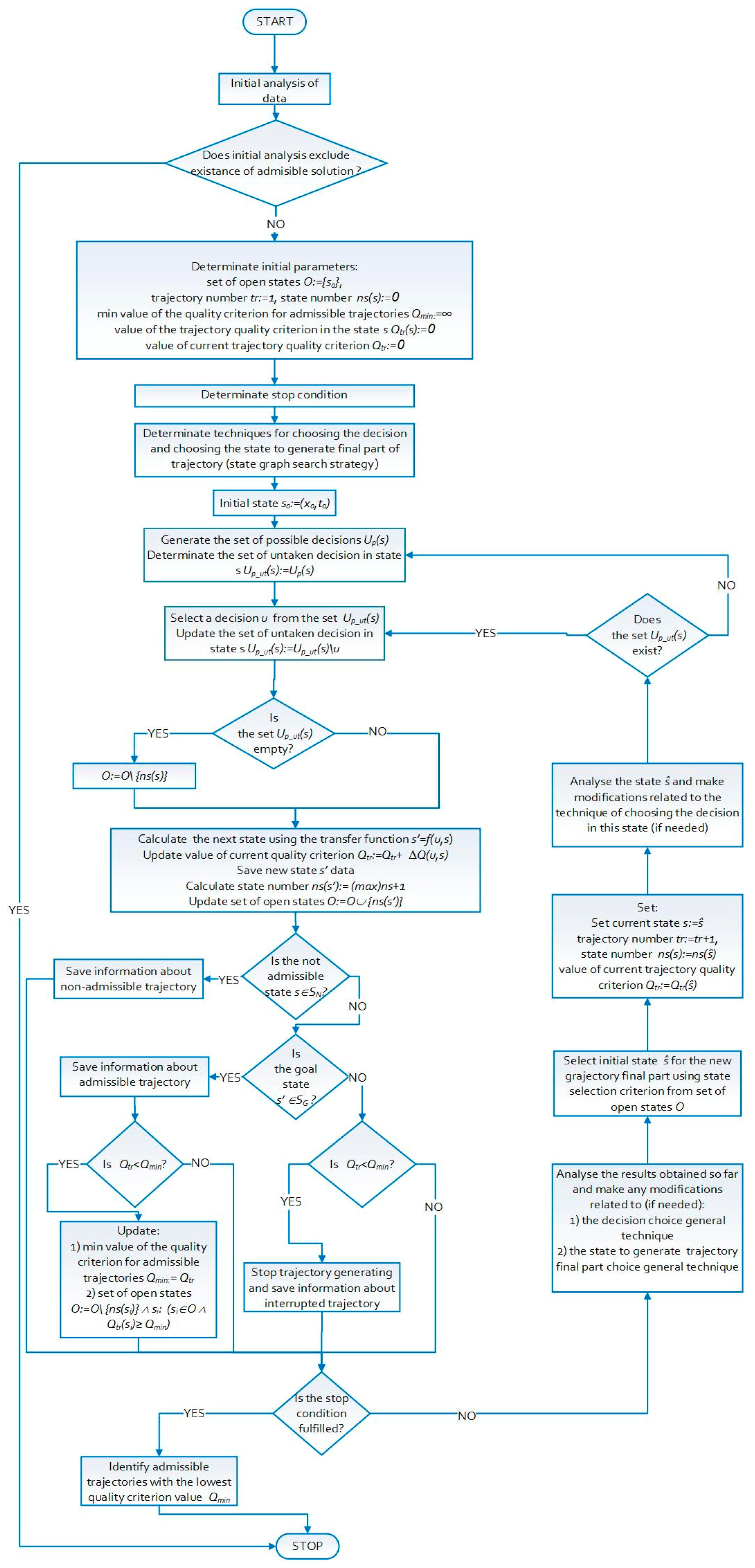
5.7. Algorithm Class Scheme

A scheme of algorithm class that generates the final parts of trajectory is presented in Figure 3. The scheme includes the components shown above integrated into the trajectory generation algorithm. The algorithm can terminate its operation when one of the following conditions is true:

• it has generated a predetermined amount of the trajectory,
• a satisfactory solution has been obtained (with a good enough quality criterion value),
• there is no significant improvement in the quality criterion value for the subsequent admissible trajectories,
• all trajectories were constructed (most often this does not happen).

As mentioned above, it is possible to find the optimal solution using this algorithm with sufficient time for calculations. However, as is known, for NP-hard problems, the computation time of the exact algorithm is not a polynomial function of the size of the problem. Because of this, the algorithm is interrupted and provides an approximate solution.

6. Sample Scheduling Problem

To illustrate the presented approach, let us consider, in a formal way, the following problem that belongs to the class described in Section 2.

We consider a project consisting of tasks (jobs) where the possibility of starting a task depends on the completion of other tasks. Thus, tasks and the relationships between them are represented by a non-directed graph G = (V,E), where V = {1, …, n} is the set of vertices and E is the set of edges. Vertex 1 is the starting point of the work. The edges represent jobs that must be performed. We consider that m executors (machines) M_j (j = 1,...,m) have to process n jobs J_i (i = 1, ..., n). The machines are in parallel and unrelated. Jobs may be processed on any of the machines. It is assumed that job splitting is not allowed, so job processing cannot be interrupted and resumed at a later time. The jobs are dependent because precedence relationships between jobs are represented by the graph G. Release dates $r_i$, at which time job J_i becomes available for processing, are defined for all jobs and depend on the previously performed jobs according to the graph G. Thus, they are dependent on process state s, and therefore they are denoted as $r_i\left(s\right)$. The deadlines for some of the jobs d(j) are given. Moreover, the production process may require a machine setup (not always for all machines). Setup cannot be interrupted before its completion. We consider that the time of setup is not known a priori and depends not only on the job sequence, but also on a set of previously performed jobs, because previously performed jobs may be used as a resource for machine setup. Resources can only be used by one machine at a time. An objective function should be specified. For example, it may be the makespan (minimum job completion time) or sum of the costs of performing a job. This problem can be treated as a problem belonging to the class of arc routing problems with deadlines and setups in which the time depends on the process state.

An example of such a complex project is the construction of a headings network in preparatory work in mines. The set of headings in the mine must be driven in order to render the exploitation field accessible. The headings form a net formally (represented by a non-oriented multigraph G = (W,C,P), where the set of branches C and the set of nodes W represent the set of headings and the set of heading crossings, respectively). The project begins at time $t_0=0$ in the initial indicated node and ends at the moment of execution of all headings. The heading can be made by an executor or working group of different efficiency and cost of performing. In particular, a specialized machine, i.e., a mining combine, is used. These working groups are more effective but their cost is much higher and a mining combine must be transported when driving starts at a different crossing than the one in which the machine is placed. A heading performing cannot be interrupted before its completion and can be done only by one working group at a time.

The task of executing headings can be started if one of the adjacent headings is made. Thus, release dates $r_i$ are not known a priori and depend on the previously performed jobs. Moreover, the formerly prepared plan of field exploitation causes due dates for some of the headings. In cases where a transport of mining combine is necessary, the shortest transportation route from the current crossing to the one from which the next heading performing should be started will be chosen. The transport route depends on the state of the whole system, since transport is possible only through completed headings. Thus, it is a problem with state-dependent resources. Moreover, this transport can be considered as machine setup.

Decisions to assign a working group to another heading performing are always made after the completion of previous work by this team and the decision takes into account the business of all working groups.

Because of the importance of cost, the optimization problem can be formulated as a determination of such an order of heading performance and their assignment to a particular working group, which would minimize the total project costs and ensure the completion of each job before its due date.

6.1. Formal Model of Problem

Based on the ALMM methodology, it is possible to build different models of the same problem. The model for the preparatory work in mines problem was proposed by Dudek-Dyduch in [28]. It differs from the one presented below because of another state system encoding. This section presents an algebraic-logical model of scheduling problems on unrelated parallel machines with deadline and machine setup dependent on the process state where relationship between tasks is defined by the graph. The model presented below is an extension and generalization of the model shown in [32]. Additionally, the details of the decision and transition function, set of possible decisions, and costs calculation are shown in detail.

The following notation is used:

• $G=\left(V,E\right)$—a non-directed graph where vertices set $V=1,2,\dots ,n$ correspond to nodes representing places where the machine starts and/or finishes performing the current job and the edge set $E=1,2,\dots ,e$ correspond to jobs,
• $M$—set of machine (working groups), $M=M_1\cup M_2$ where $M_1$—subset of machine (working groups) for which setup is required and $M_2$—subset of machine (working groups) that does not require setup,
• $J$—set of jobs.

The process state at any instant $t$ is defined as a vector $x=\left(x^0,x^1,\dots ,x^{\left|M\right|}\right)$, where $M=M_1\cup M_2$. A coordinate $x^0$ describes a set of jobs that have been performed up to moment $t$. The other coordinate $x^m$ describes the state of the $m$-th machine, where $m=1,2,\dots ,\left|M\right|$. The structure of the machine state is as follows $x^m=\left(p,\omega ,\lambda \right)$, where

• $p\in J\cup \left\{0\right\}$—represents the number of the job assigned to the $m$-th machine to perform; 0 denotes that a job is not assigned to any machine.
• $\omega \in V$—the number of the node where the machine is located or the number of the node in which it finishes performing the assigned job $j$;
• $\lambda \in [0,\infty )$—the length of the route that remains to reach the node $\omega =v$ by the $m$-th machine (in particular, $\lambda >l\left(j\right)$ means the machine setup; the value $\lambda$ is the sum of the $l\left(j\right)$ length of job $j$ assigned to the $m$-th machine and the length of the route until the transportation is finished).

The initial state $s_0=\left(x_0,t_0\right)$ of the system is as follows: $x_0=\left(x_0^0,x_0^1,\dots ,x_0^{\left|M\right|},\right), t_0=0$. All jobs are incomplete, so the set $x_0^0$ is an empty set $x_0^0=\varnothing$. In addition, no job is assigned to the machines and all machines are in the initial node. So the initial state of each machine is $x_0^m=\left(0,0,0\right)$ for $m=1,2,\dots ,\left|M\right|$.

A state $s=\left(x,t\right)$ belongs to the set of non-admissible states if there is a job that is not complete yet and its due date is earlier than $t$. The definition $S_N$ is as follows (where $d(j)$ denotes the due date for the job j):

$$S_N=s\left(x,t\right):\left(\exists j\in J,j\notin x^0\right){\displaystyle \bigwedge }d\left(j\right)<t\}.$$

(2)

A state $s=\left(x,t\right)$ is a goal if all the jobs have been performed before the deadline. The definition of the set of goal states $S_G$ is as follows:

$$S_G=s\left(x,t\right):\left(\forall j\in J,j\notin x^0\right){\displaystyle \bigwedge }d\left(j\right)\ge t\}.$$

(3)

Let us distinguish the following characteristic classes of machine states m, useful in building the other components of the problem model:

• $X_I^m$ is a set that corresponds to the situations where the machine is in the node:

  $$X_I^m=\{\left(p,\omega ,\lambda \right):p=0{\displaystyle \bigwedge }\omega \in V{\displaystyle \bigwedge }\lambda =0\}.$$

  (4)
• $X_{II}^m$ is a set that corresponds to situations where machine $m$ is performing job $j$ toward node $v_f\left(j\right)$:

  $$X_{II}^m=\{\left(p,\omega ,\lambda \right):p=j{\displaystyle \bigwedge }\omega =v_f\left(j\right){\displaystyle \bigwedge }\lambda \in (0,l\left(j\right)]\}.$$

  (5)
• $X_{III}^m$ is a set that corresponds to situations where machine $m\in M1$ is transported to job $j$ and will perform it toward node $v_f\left(j\right)$:

  $$X_{III}^m=\{\left(p,\omega ,\lambda \right):p=j{\displaystyle \bigwedge }\omega =v_f\left(j\right){\displaystyle \bigwedge }\lambda \in (l\left(j\right),\infty ]\}.$$

  (6)

The decision $u=\left(u^1,u^2,\cdots ,u^{\left|M\right|}\right)$ is taken together for all machines. It determines which job or jobs should be started at moment t, which machines are assigned to perform the jobs, which machines should be set up, and which machines should wait. The particular coordinate $u^m$ refers to the $m$-th machine and $u^m=J\cup \left\{0\right\}$, where $u^m=j$ denotes that job $j$ is assigned to be performed by machine $m$ and $u^m=0$ denotes a continuation of the previous machine operations. The only possible decision can be taken in the given state $s=\left(x,t\right)$. It is impossible to start performing a job when no job represented by the adjacent edge in graph $G$ is completed. Also, it is impossible to assign a new job to a machine that is currently continuing a previously assigned job (setup or performing job). Moreover, it may be decided to stop a machine or machines if at least one machine is currently working or has a job assigned.

Thus, the set of possible decisions in the state $s=\left(x,t\right)$ is:

$$U_p\left(s\right)=U_p^1\left(s\right)\times U_p^2\left(s\right)\times \cdots \times U_p^{\left|M\right|}\left(s\right)\backslash H\left(s\right).$$

(7)

The set of possible decisions $U_p^m$(s) for the $m$-th machine in the state $s=\left(x,t\right)$ is defined as follows:

$${\forall }_{m=1,2,..,\left|M\right|}{U}_p^m\left(s\right)=\{\begin{array}{cc}{J}_D\left(s\right)\cup \left\{0\right\}& form:x^m\left(s\right)\in X_I^m\\ \left\{0\right\}& form:x^m\left(s\right)\in \left(X_{II}^m\cup X_{III}^m\right)\end{array},$$

(8)

where $J_D\left(s\right)$ denotes a set of jobs that are available in a given state, including jobs that are unperformed and not assigned to any machine, and for which there is a transport path.

H(s) denotes the set of decisions to assign one job to be performed by more than one machine and decisions not to assign any jobs to be performed by any machine when all the machines in a given state are standing. The set $H\left(s\right)$ definition is as follows:

$$H\left(s\right)=\{u:\left({\exists }_{i,j=1,2,\dots ,\left|M\right|,i\ne j}{u}^i\left(s\right)=u^j\left(s\right)\ne 0\right){\displaystyle \bigvee }\left({\forall }_{i=1,2,\dots ,\left|M\right|}{u}^i\left(s\right)=0\wedge x^i\left(s\right)\in X_I^m\right)\}.$$

(9)

The decision $u=\left(u^1,u^2,\cdots ,u^{\left|M\right|}\right)$ is non-admissible when it leads to the state $s=\left(x,t\right)$ belonging to the set $S_N$, i.e., as a result of the decision $d\left(j\right)$ is exceeded for a job.

Based on the current state $s=\left(x,t\right)$ and the decision $u$ taken in this state, the subsequent state $\left(x’,t’\right)=f\left(u,x,t\right)$ is generated by means of the transition function $f$.

Firstly, the moment $t’$ is determined. This is the nearest moment at which at least one machine will finish its work. For that purpose, $t_m$ time of completion of the realized task needs to be calculated for each machine. The subsequent state will occur in the moment $t^{\prime }=t+∆t$, where $∆t$ equals the lowest value of the established set of $t_m$. The next state occurs at the moment $t^{\prime }=t+∆t$, where $∆t=mi{n}_{m=1,2,\dots ,\left|M\right|}{t}_m$. Let $\left|r_{min}\left(m,j\right)\right|$ denote the length of the shortest transportation route to job $j$ for machine $m$, $V_P^m$ denote the efficiency of m machine (performing length per time unit) and $V_S^m$ denote the speed of the machine setup. The completion time $t_m$ for the machine $m$ in a given state $s$ depends on the type of decision and equals:

• the sum of the setup time (transport by the shortest transport route of $\left|r_{min}\left(m,j\right)\right|$ length at a $V_S^m$ speed) and the job completion time (performing job $j$ of $l\left(j\right)$ length at speed $V_P^m$) when machine $m\in M_1$ is standing in node v.
• the job j completion time (performing job $j$ of $l\left(j\right)$ length at speed $V_P^m$) when the machine $m\in M_2$ is standing in node $v$.
• the completion time remaining $\lambda \le l\left(j\right)$ length at speed $V_P^m$ when machine $m\in M$ continues processing the previously assigned job.
• the sum of the setup time remaining $\lambda -l\left(j\right)$ length at speed $V_S^m$ and the job $j$ completion time (performing job $j$ of $l\left(j\right)$ length at speed $V_P^m$) when machine $m\in M_1$ continues processing the previously assigned job and is in the process of setup.
• if the machine is standing in node $v$ and no decision has been made to assign another job, then the completion time equals infinity.

Thus, the completion time $t_m$ can be represented in the following form:

$$t_m=\{\begin{array}{cc}\frac{\left|r_{min}\right(m,j\left)\right|}{V_S^m}+\frac{l\left(j\right)}{V_P^m}& :x^m\in X_I^m\wedge u^m\left(s\right)=j\wedge m\in M_1\\ \frac{l\left(j\right)}{V_P^m}& :x^m\in X_I^m\wedge u^m\left(s\right)=j\wedge m\in M_2\\ \frac{\lambda }{V_P^m}& :x^m\in X_{II}^m\wedge u^m\left(s\right)=0\\ \frac{\lambda -l\left(j\right)}{V_S^m}+\frac{l\left(j\right)}{V_P^m}& :x^m\in X_{III}^m\wedge u^m\left(s\right)=0\\ \infty & :x^m\in X_I^m\wedge u^m\left(s\right)=0\end{array}.$$

(10)

Once the moment $t’$ is known, it is possible to determine the proper state of the process at the time.

The first coordinate $x^0$ of the proper state, i.e., the set of completed jobs, is increased by the number of jobs that have been finished at moment $t’$:

$$x^{0\text{'}}=x^0\cup \{j:{\exists }_{m\in M}{x}^m\left(s\right)=\left(p,\omega ,\lambda \right){\displaystyle \bigwedge }p=j{\displaystyle \bigwedge }{t}_m=∆t\}.$$

(11)

Afterwards, the values of subsequent coordinates in the new state are determined by $x^m\text{'}=\left(p^{\prime },{\omega }^{\prime },{\lambda }^{\prime }\right)$, for m = 1,2…|M|, which represent the states of particular machines. Particular parameters of the coordinate of the new machine state are determined as described in

Table 1. Particular parameters of the coordinate of the new machine state.

for the Decision to Continue the Activity of the Machine ${\mathit{u}}^{\mathit{m}}=0$:

$p^{\prime }=\{\begin{array}{cc}p& :t_m>∆t\\ 0& :t_m=∆t\end{array}$

${\omega }^{\prime }=\omega$

${\lambda }^{\prime }=\{\begin{array}{cc}\lambda -V_S^m\cdot min\left(\frac{max\left(\lambda -l\left(j\right),0\right)}{ V_S^m},∆t\right)-V_P^m\cdot max\left(∆t-\frac{max\left(\lambda -l\left(j\right),0\right)}{ V_S^m},0\right)& :m\in M_1\\ \lambda - V_P^m\cdot ∆t& :m\in M_2\end{array}$

for the Decision to Assign a New Task to the Machine ${\mathit{u}}^{\mathit{m}}=\mathit{j}$:

$p^{\prime }=\{\begin{array}{cc}j& :t_m>∆t\\ 0& :t_m=∆t\end{array}$

${\omega }^{\prime }=v_f\left(j\right)$

${\lambda }^{\prime }=\{\begin{array}{cc}\left|r_{min}\left(m,j\right)\right|+l\left(j\right)-V_S^m\cdot min\left(\frac{\left|r_{min}\left(m,j\right)\right|}{ V_S^m},∆t\right)-V_P^m\cdot max\left(∆t-\frac{\left|r_{min}\left(m,j\right)\right|}{ V_S^m},0\right)& :m\in M_1\\ l\left(j\right)-V_P^m\cdot ∆t& :m\in M_2\end{array}$

, where $v_f\left(j\right)$ is the node adjacent to job $j$, in which the machine will finish.

Determining the value of the quality criterion is as follows. The task of optimization consists of minimizing all the costs of performing the work. Thus the quality criterion denotes the total cost of the work, which is the sum of the costs of decisions taken in the multistage decision process. The property of the criterion’s separability allows for its recursive calculation.

In a given state $s_{k+1}$, the total cost of work from initial state to that state is the sum of the costs in the previous state $s_k$ and the increment of the costs of executing decision $u_k$ taken in the state $s_k$: $Q_{k+1}=Q_k+∆Q_k\left(u_k,s_k\right)$. The cost increase is the sum of the costs of using individual machines, which is the result of the type of machine activity (standing, performing, and setup).

Table 2. Cost increase for machine m.

for the Decision to Continue the Activity of the Machine ${\mathit{u}}^{\mathit{m}}=0$:
$∆Q^m\left(u_k^m,s_k\right)=\{\begin{array}{cc}{K}_{STOP}^m\cdot ∆t& :x_m\in X_I^m{\displaystyle \bigwedge }m\in M\\ K_P^m\cdot ∆t& :x_m\in X_{II}^m{\displaystyle \bigwedge }m\in M_2\\ K_S^m\cdot min\left(\frac{\left|r_{min}\left(m,j\right)\right|}{ V_S^m},∆t\right)+K_P^m\cdot max\left(∆t-\frac{\left|r_{min}\left(m,j\right)\right|}{ V_P^m},0\right)& :x_m\in X_{II}^m\cup X_{III}^m{\displaystyle \bigwedge }m\in M_1\end{array}$
for the Decision to Assign a New Task to the Machine ${\mathit{u}}^{\mathit{m}}=\mathit{j}$:
$∆Q^m\left(u_k^m,s_k\right)=\{\begin{array}{cc}{K}_S^m\cdot min\left(\frac{\left|r_{min}\left(m,j\right)\right|}{ V_S^m},∆t\right)-K_P^m\cdot max\left(∆t-\frac{\left|r_{min}\left(m,j\right)\right|}{ V_P^m},0\right)& :m\in M_1\\ K_P^m\cdot ∆t& :m\in M_2\end{array}$

presents the cost increase for machine m, where $K_{STOP}^m$ denotes the unit cost of m machine standing, $K_P^m$ denotes the unit cost of m machine performing, and $K_S^m$ denotes the unit cost of m machine setup.

6.2. Algorithm

The algorithms based on the algebraic-logic model were developed for the problem under consideration. The corresponding algorithm for generating a single trajectory is described in [32,33]. Its components have been partially used in the algorithms below that generate the final part of the trajectory.

The basic components of the presented algorithms are as follows:

• preliminary analysis of data—firstly, it is verified that an admissible solution exists or the time limitation is active for the given problem. Secondly, some characteristic features of the problem have been identified, i.e., a deadline for some jobs, and a much higher cost of using machines with setup. They were used to determine the form of local optimization and attributes of state graph node selection.
• local choice—the decision in the given state is chosen using the special local optimization task with semimetrics. Three versions of the local decision criterion are presented below.
  Criterion q1 is as follows. The local criterion takes into account a component related to the cost of the work, a component related to the necessity for the trajectory to omit the states of set $S_N$ (each job is completed before its due date) and a component for preferring some cooperative decisions. Thus, the local criterion is of the form ($a_1,b_1,b_2$—weights of particular components):

  $$q1\left(u,x,t\right)=∆Q\left(u,x,t\right)+{\widehat{Q}}_1\left(u,x,t\right)+a_1{E}_1\left(u,x,t\right)+b_1{F}_1\left(u,x,t\right)+b_2{F}_2\left(u,x,t\right),$$

  (12)

  where $∆Q\left(u,x,t\right)$ denotes the increase of work cost, calculated as described in Table 2. ${\hat{Q}}_1\left(u,x,t\right)$ is the estimated cost of finishing unperformed jobs (connected with the final section of the trajectory) and is calculated as the sum of the costs of completing decisions made earlier (performing job and/or setup machines), the cost of performing unperformed jobs by the cheapest machine, and the cost of other machines’ stopover. The third component $E_1\left(u,x,t\right)$ uses the value of the estimated “distance” between the new potential state $s_{p\_k}$, and the set of non-admissible states. The time reserve $r_{tc}\left(s_{p\_k}\right)=d\left(j\right)-t_{p\_k}-\tau \left(j\right)-t_{end}$ for each unfinished or unassigned job j with a due date is calculated and takes into consideration $d\left(j\right)$ due date for job $j$, $\tau \left(j\right)$ time necessary to perform job $j$ and unperformed jobs forming the shortest path by the fastest machine, and $t_{end}$ time necessary to finalize the fastest machine current activity. $E_1\left(u,x,t\right)$ is inversely proportional to the minimum value of time reserve $r_{tc}\left(s_{p\_k}\right)$ for its values greater than 0, and equals to 0 otherwise. The component $F_1\left(u,x,t\right)$ is responsible for preferring the first type of co-operation decisions, i.e., a reduction of machine idleness time in order to perform transport, especially if there are due dates. It is calculated as a penalty for a decision about a stopover in a case where a machine could have started another job. The component $F_2\left(u,x,t\right)$ is responsible for preferring the second type of co-operation decisions, i.e., assigning only the cheapest machines to perform jobs in case the time limits are no longer active. It is calculated as a penalty for a decision to have a job performed by other machines than the lowest-cost ones when all jobs with a due date have been finished.
  Criterion q2 is as follows. The form of the criterion as well as the form above takes into account a component related to the cost of work, a component related to necessity for the trajectory to omit the states of set $S_N$ (each job is completed before its due date), and components for preferring some co-operation decisions. However, the three components are determined in different ways. First, the exact increase of work cost, instead of being calculated, is estimated. Estimation $∆Q\left(u,x,t\right)$ is equal to the sum of costs of execution of unfinished and unstarted earlier jobs that are chosen to be performed by machines in a given decision and cost of transport of machines (the machine’s standing cost is omitted). Secondly, the estimated cost ${\widehat{Q}}_2\left(u,x,t\right)$ of finishing unperformed jobs (connected with the final section of the trajectory) is calculated as the sum of the cost of performing the unfinished and unstarted earlier jobs by the cheapest machine (machine) and the cost of other standing machines. Thirdly, component $E_2\left(u,x,t\right)$ is a minimum value of the sum of the shortest path to a job with deadline with these job’s lengths. It is determined only for a job with a deadline that is neither finished nor started earlier nor under consideration to be performed by machines in a given decision. Finally, criterion q2 is as follows:

  $$q2\left(u,x,t\right)=∆Q\left(u,x,t\right)+{\widehat{Q}}_2\left(u,x,t\right)+a_1{E}_2\left(u,x,t\right)+b_1{F}_1\left(u,x,t\right)+b_2{F}_2\left(u,x,t\right).$$

  (13)
  Criterion q3 is as follows. The third criterion version differs from the second way of determining the component $E\left(u,x,t\right)$. It is close to the average value of time reserves r_tc(s_{p_k}) for values greater than 0 and equals to 0 otherwise. Criterion q3 is as follows:

  $$q3\left(u,x,t\right)=∆Q\left(u,x,t\right)+{\widehat{Q}}_2\left(u,x,t\right)+a_1{E}_3\left(u,x,t\right)+b_1{F}_1\left(u,x,t\right)+b_2{F}_2\left(u,x,t\right).$$

  (14)
• Modification of local search—the first type of modification consists of changing the $a_1,b_1,b_2$ coefficients value after the generation of a trajectory. If it is non-admissible, then for the subsequent trajectory, the value of weight $a_1$ should be increased because of the distance from the set of non-admissible states. The increase of the weight $b_1$ value, which would result in lower probability of a machine stopover, can also be helpful. If the generated trajectory is admissible, then for the subsequent trajectory the values of the coefficients may be decreased and the weight of the components related to the execution cost should be increased. The second modification type consists of changing the local optimization form during trajectory generation. When all jobs with due dates are finished, there is no need to specify “distance” between the state and the set of non-admissible states. Thus, it is no longer necessary to apply the component $E\left(u,x,t\right)$ in the local criterion and the modified criterion is as follows:

  $$q\left(u,x,t\right)=∆Q\left(u,x,t\right)+{\widehat{Q}}_2\left(u,x,t\right)+b_1{F}_1\left(u,x,t\right)+b_2{F}_2\left(u,x,t\right).$$

  (15)
• the pruning of non-perspective parts of trajectory—a trajectory generation or its finished part is interrupted when in the newly generated state we obtain a quality index that is worse than the quality index for the best solution. The information gained as a result of the trajectory analysis is used to modify the local optimization task for the next trajectory.
• selection of state graph node—on the basis of the problem analysis, characteristic parameters were determined: cost of jobs performing for the initial part of the trajectory, total length of part. The initial state for the trajectory final part may be the state in which:
  • the ratio of the cost of jobs’ performance for the initial trajectory to the total length of performed jobs is the smallest (attribute denoted by $\widehat{s1}$);
  • the ratio of the cost of jobs’ performance for the initial trajectory to the current state time is the smallest (attribute denoted by $\widehat{s2}$);
  • the ratio of the total length of performed jobs to the current state time e is the smallest (attribute denoted by $\widehat{s3}$);
  • the minimum time reserve for unperformed jobs with a due date is the highest (attribute denoted by $\widehat{s4}$);
  • the ratio of the minimum time reserve for unperformed jobs with a due date to the total length of performed jobs is the highest (attribute denoted by $\widehat{s5}$).

7. Experimental Results

The purpose of the current experiments was to examine the efficiency of algorithms that generate multiple trajectories, using the ability to improve the obtained solution by changing the final part of the trajectory. For this purpose, the simulation experiments were carried out involving the construction of 40 trajectories (or trajectory final part) with the use of a specific criterion for the selection of local decisions, the modifications of the local decision search described above, the pruning of non-perspective parts of the trajectory, and the five ways described above to choose the state from which the final part of the trajectory is generated. Examples were selected so that the existence of an admissible solution could not be ruled out. A verification of the effectiveness of the proposed form of local criterion and applying the components $E\left(u,x,t\right)$ and $F\left(u,x,t\right)$ was carried out and shown in [32,33].

The research was conducted for the set of four regular structure heading networks (denoted as GR) and five irregular structure heading networks (denoted as GIr). Each network is represented by a planar graph, in which the vertex degrees equal 1 to 4. The number of jobs with a deadline was approximately 25% of all jobs. Parameters of relevant heading networks (number of node, number of edge, and total length of jobs to perform) are presented in

Table 3. Network data.

Problem Example	GR-1a	GR-1b	GR-2	GR-3	GIr-1	GIr-2	GIr-3	GIr-4	GIr-5
Number of node	20	20	20	20	24	27	27	29	67
Number of edge	18	18	18	18	20	20	20	20	50
Total length to perform	1008	1008	1010	1066	1364.45	1863.07	1863.07	1869.88	4579.11

. The tasks were performed by one machine (working groups) for which setup is required and one machine (working groups) that does not require setup. The parameters of the first machine were as follows: performing speed 10.0 m/h, setup speed 100 m/h, performing cost 200.0 $/h, transport cost 100.0 $/h and standing cost 30.0 $/h. The parameters of the second machine were as follows: performing speed 5.0 m/h, performing cost 50.0 $/h and standing cost 5.0 $/h. Table 3 presents data for all networks.

Experiments were conducted as follows. Three groups of algorithms were tested; the first one used the criterion q1 (Equation (8)) to select the decision in a given state, the second criterion q2, and the third criterion q3. The values of the component coefficients in the local criterion q1, q2, and q3 were selected on the basis of previous results obtained for algorithms generating single whole trajectories. In each algorithm group we used the selection of state graph node method, i.e., $\widehat{s1}$, $\widehat{s2}$, $\widehat{s3}$, $\widehat{s4}$, and $\widehat{s5}$. The brutal force algorithm was used to obtain an optimal solution and check the effectiveness of the mentioned algorithms. However, the optimal solution was obtained for one network only, namely GR-2. In other cases, the simulation calculation was stopped after about two days, since the time for obtaining a solution was not effective and for real decision-making it was too long. After this time of calculation, suboptimal solutions for GR-1a, GR-1b, GR-3, GIr-1, and GIr-4 were obtained. For the remaining networks, an admissible solution was not found.

Table 3,

Table 4. Obtained results for regular network GR-1a (Suboptimal cost 16,480.00).

Problem Example	Obtained Total Cost	Percentage Error	Simulation Time (ms)
Alg. q1	16,922.00	2.682%	296
Alg. $q1-\widehat{s1}$	16,957.70	2.899%	390
Alg. $q1-\widehat{s2}$	17,026.90	3.319%	203
Alg. $q1-\widehat{s3}$	16,894.30	2.514%	515
Alg. $q1-\widehat{s4}$	16,957.70	2.899%	437
Alg. $q1-\widehat{s5}$	16,957.70	2.899%	437
Alg. q2	16,811.90	2.014%	140
Alg. $q2-\widehat{s1}$	16,741.30	1.586%	187
Alg. $q2-\widehat{s2}$	16,741.30	1.586%	125
Alg. $q2-\widehat{s3}$	16,811.90	2.014%	171
Alg. $q2-\widehat{s4}$	16,730.70	1.163%	140
Alg. $q2-\widehat{s5}$	16,730.70	1.521%	203
Alg. q3	16,855.80	2.280%	187
Alg. $q3-\widehat{s1}$	16,613.80	0.812%	187
Alg. $q3-\widehat{s2}$	16,710.30	1.397%	93
Alg. $q3-\widehat{s3}$	16,873.70	2.389%	187
Alg. $q3-\widehat{s4}$	16,710.30	1.397%	125
Alg. $q3-\widehat{s5}$	16,710.30	1.397%	187

,

Table 5. Obtained results for regular network GR-1b (Suboptimal cost 16,538.30).

Problem Example	Obtained Total Cost	Percentage Error	Simulation Time (ms)
Alg. q1	-	-	-
Alg. $q1-\widehat{s1}$	-	-	-
Alg. $q1-\widehat{s2}$	-	-	-
Alg. $q1-\widehat{s3}$	17,008.60	2.844%	984
Alg. $q1-\widehat{s4}$	-	-	-
Alg. $q1-\widehat{s5}$	-	-	-
Alg. q2	16,811.90	1.654%	187
Alg. $q2-\widehat{s1}$	16,596.00	0.349%	187
Alg. $q2-\widehat{s2}$	16,644.70	0.643%	125
Alg. $q2-\widehat{s3}$	16,811.90	1.654%	187
Alg. $q2-\widehat{s4}$	16,730.70	1.163%	140
Alg. $q2-\widehat{s5}$	16,644.70	0.643%	187
Alg. q3	17,043.80	3.056%	203
Alg. $q3-\widehat{s1}$	16,835.80	1.799%	171
Alg. $q3-\widehat{s2}$	16,835.80	1.799%	140
Alg. $q3-\widehat{s3}$	17,046.80	3.075%	109
Alg. $q3-\widehat{s4}$	16,982.90	2.688%	140
Alg. $q3-\widehat{s5}$	16,835.80	1.799%	171

,

Table 6. Obtained results for regular network GR-2 (Optimal cost 16,524.40).

Problem Example	Obtained Total Cost	Percentage Error	Simulation Time (ms)
Alg. q1	17,284.10	4.597%	265
Alg. $q1-\widehat{s1}$	17,284.10	4.597%	343
Alg. $q1-\widehat{s2}$	17,284.10	4.597%	218
Alg. $q1-\widehat{s3}$	17,139.70	3.724%	859
Alg. $q1-\widehat{s4}$	17,202.00	4.101%	375
Alg. $q1-\widehat{s5}$	17,023.40	3.020%	421
Alg. q2	16,792.20	1.621%	171
Alg. $q2-\widehat{s1}$	16,780.80	1.552%	187
Alg. $q2-\widehat{s2}$	16,780.80	1.552%	156
Alg. $q2-\widehat{s3}$	16,792.20	1.621%	93
Alg. $q2-\widehat{s4}$	16,766.00	1.462%	125
Alg. $q2-\widehat{s5}$	16,766.00	1.462%	171
Alg. q3	16,748.20	1.354%	156
Alg. $q3-\widehat{s1}$	16,653.70	0.782%	187
Alg. $q3-\widehat{s2}$	16,748.20	1.354%	156
Alg. $q3-\widehat{s3}$	16,748.20	1.354%	187
Alg. $q3-\widehat{s4}$	16,748.20	1.354%	140
Alg. $q3-\widehat{s5}$	16,748.20	1.354%	156

,

Table 7. Obtained results for regular network GR-3 (Suboptimal cost 17,448.90).

Problem Example	Obtained Total Cost	Percentage Error	Simulation Time (ms)
Alg. q1	16,359.90	−6.241%	343
Alg. $q1-\widehat{s1}$	16,359.90	−6.241%	234
Alg. $q1-\widehat{s2}$	16,359.90	−6.241%	218
Alg. $q1-\widehat{s3}$	16,176.90	−7.290%	562
Alg. $q1-\widehat{s4}$	16,359.90	−6.241%	312
Alg. $q1-\widehat{s5}$	16,359.90	−6.241%	562
Alg. q2	-	-	-
Alg. $q2-\widehat{s1}$	15,147.50	−13.189%	187
Alg. $q2-\widehat{s2}$	15,147.50	−13.189%	140
Alg. $q2-\widehat{s3}$	15,409.30	−11.689%	187
Alg. $q2-\widehat{s4}$	15,409.80	−11.689%	125
Alg. $q2-\widehat{s5}$	15,147.50	−13.189%	171
Alg. q3	16,282.10	−6.687%	171
Alg. $q3-\widehat{s1}$	15,037.80	−13.818%	140
Alg. $q3-\widehat{s2}$	15,251.90	−12.591%	156
Alg. $q3-\widehat{s3}$	15,660.70	−10.248%	171
Alg. $q3-\widehat{s4}$	15,514.20	−11.088%	125
Alg. $q3-\widehat{s5}$	15,251.90	−12.591%	187

,

Table 8. Obtained results for irregular network GIr-1 (Suboptimal cost 23,132.40).

Problem Example	Obtained Total Cost	Percentage Error	Simulation Time (ms)
Alg. q1	22,665.17	−2.020%	703
Alg. $q1-\widehat{s1}$	22,254.78	−3.794%	3171
Alg. $q1-\widehat{s2}$	22,254.78	−3.794%	1906
Alg. $q1-\widehat{s3}$	22,288.02	−3.650%	3062
Alg. $q1-\widehat{s4}$	22,288.02	−3.650%	2812
Alg. $q1-\widehat{s5}$	22,665.17	−2.020%	203
Alg. q2	22,336.91	−3.439%	390
Alg. $q2-\widehat{s1}$	22,194.99	−4.052%	343
Alg. $q2-\widehat{s2}$	22,194.99	−4.052%	343
Alg. $q2-\widehat{s3}$	22,215.28	−3.965%	359
Alg. $q2-\widehat{s4}$	22,215.28	−3.965%	281
Alg. $q2-\widehat{s5}$	22,194.99	−4.052%	359
Alg. q3	22,274.50	−3.709%	296
Alg. $q3-\widehat{s1}$	22,204.96	−4.009%	437
Alg. $q3-\widehat{s2}$	22,204.96	−4.009%	375
Alg. $q3-\widehat{s3}$	22,204.96	−4.009%	437
Alg. $q3-\widehat{s4}$	22,204.96	−4.009%	390
Alg. $q3-\widehat{s5}$	22,204.96	−4.009%	437

,

Table 9. Obtained results for irregular network GIr-2 (suboptimal cost).

Problem Example	Obtained Total Cost	Percentage Error	Simulation Time (ms)
Alg. q1	30,946.33	-	937
Alg. $q1-\widehat{s1}$	30,942.21	-	2812
Alg. $q1-\widehat{s2}$	30,946.33	-	1421
Alg. $q1-\widehat{s3}$	30,946.33	-	781
Alg. $q1-\widehat{s4}$	30,942.21	-	3187
Alg. $q1-\widehat{s5}$	30,946.33	-	1156
Alg. q2	30,557.18	-	609
Alg. $q2-\widehat{s1}$	30,538.75	-	250
Alg. $q2-\widehat{s2}$	30,538.75		250
Alg. $q2-\widehat{s3}$	30,538.75	-	281
Alg. $q2-\widehat{s4}$	30,538.75	-	250
Alg. $q2-\widehat{s5}$	30,538.75	-	265
Alg. q3	30,589.50	-	531
Alg. $q3-\widehat{s1}$	30,348.72	-	343
Alg. $q3-\widehat{s2}$	30,348.72	-	343
Alg. $q3-\widehat{s3}$	30,640.40	-	343
Alg. $q3-\widehat{s4}$	30,459.47	-	312
Alg. $q3-\widehat{s5}$	30,640.40	-	281

,

Table 10. Obtained results for irregular network GIr-3 (suboptimal cost).

Problem Example	Obtained Total Cost	Percentage Error	Simulation Time (ms)
Alg. q1	30,888.34	-	937
Alg. $q1-\widehat{s1}$	31,118.46	-	2437
Alg. $q1-\widehat{s2}$	31,118.46	-	1953
Alg. $q1-\widehat{s3}$	31,118.46	-	328
Alg. $q1-\widehat{s4}$	30,867.65	-	2171
Alg. $q1-\widehat{s5}$	31,118.46	-	609
Alg. q 2	30,678.03	-	468
Alg. $q2-\widehat{s1}$	30,585.75	-	453
Alg. $q2-\widehat{s2}$	30,585.75	-	453
Alg. $q2-\widehat{s3}$	30,745.29	-	500
Alg. $q2-\widehat{s4}$	30,605.05	-	453
Alg. $q2-\widehat{s5}$	30,435.21	-	468
Alg. q3	30,853.40	-	531
Alg. $q3-\widehat{s1}$	30,688.69	-	421
Alg. $q3-\widehat{s2}$	30,688.69	-	390
Alg. $q3-\widehat{s3}$	30,728.81	-	437
Alg. $q3-\widehat{s4}$	30,616.40	-	421
Alg. $q3-\widehat{s5}$	30,616.40	-	390

,

Table 11. Obtained results for irregular network GIr-4 (Suboptimal cost 31,142.54).

Problem Example	Obtained Total Cost	Percentage Error	Simulation Time (ms)
Alg. q1	30,662.32	−1.542%	2250
Alg. $q1-\widehat{s1}$	30,662.32	−1.542%	2593
Alg. $q1-\widehat{s2}$	30,662.32	−1.542%	1437
Alg. $q1-\widehat{s3}$	30,611.50	−1.705%	5515
Alg. $q1-\widehat{s4}$	30,662.32	−1.542%	1578
Alg. $q1-\widehat{s5}$	30,662.32	−1.542%	5781
Alg. q2	30,628.30	−1.651%	1046
Alg. $q2-\widehat{s1}$	30,741.57	−1.287%	234
Alg. $q2-\widehat{s2}$	30,741.57	−1.287%	218
Alg. $q2-\widehat{s3}$	30,741.57	−1.287%	328
Alg. $q2-\widehat{s4}$	30,741.57	−1.287%	218
Alg. $q2-\widehat{s5}$	30,741.57	−1.287%	203
Alg. q3	31,255.60	0.363%	328
Alg. $q3-\widehat{s1}$	30,924.39	−0.700%	343
Alg. $q3-\widehat{s2}$	30,924.39	−0.700%	328
Alg. $q3-\widehat{s3}$	30,924.39	−0.700%	421
Alg. $q3-\widehat{s4}$	30,924.39	−0.700%	328
Alg. $q3-\widehat{s5}$	30,924.39	−0.700%	328

and

Table 12. Obtained results for irregular network GIr-5 (suboptimal cost).

Problem Example	Obtained Total Cost	Percentage Error	Simulation Time (ms)
Alg. q1	77,288.44	-	9546
Alg. $q1-\widehat{s1}$	77,288.44	-	20,171
Alg. $q1-\widehat{s2}$	77,288.4	-	15,921
Alg. $q1-\widehat{s3}$	77,146.08	-	23,906
Alg. $q1-\widehat{s4}$	77,146.08	-	23,687
Alg. $q1-\widehat{s5}$	77,288.44	-	22,234

present the results obtained for a particular network. “Alg. $q1-\widehat{s3}$” denotes an algorithm with the criterion q1 for decision selection and choice of the node for generating the final part of the trajectory, by $\widehat{s1}$ for example. The tables show the best obtained cost, percentage error, and simulation time (in milliseconds) for particular algorithms. Based on the results obtained, it can be stated that the calculation time for these algorithms is not even 1 s, and for the largest network it is up to 24 s. The resulting objective function values (total cost of work) are also good. For the GR-2 network (with a known optimal solution), the maximum percentage error was 4.597%, and the best result was obtained for algorithm $q3-\widehat{s1}$, for which the solution varied by just 0.782%. For the GR-1a, GR-1b, GR-3, GIr-1, and GIr-4 networks, the total cost was less than the obtained suboptimal cost. This is confirmed by the percentage error value (the largest difference in favor of the presented algorithms was 13.818% for the GR-3 network). It can be concluded that for regular networks the algorithm that is the combination of the selection criteria q3 and node $\widehat{s1}$ gives the best results. However, the same trend does not apply to irregular networks. The tests were performed under uniform simulated conditions, and the algorithms did not resolve all networks (Alg. $q1-\widehat{s1}$, $q1-\widehat{s2}$, $q1-\widehat{s4}$, and $q1-\widehat{s5}$ for the GR-1b network, and Alg. $q2-\widehat{s1}$ for the GIr-5 network). At the same time, there are no solutions for an algorithm that generates single whole trajectories. On the other hand, it is important to note that in some cases algorithms generating final part of trajectories have found a solution (Alg. q1 for GR-1b and Alg. q2 for GR-3) with suboptimal cost while the algorithm generated independently of whole trajectories did not find any admissible solutions.

Table 13. Summary of obtained results.

Problem Example	GR-1a	GR-1b	GR-2	GR-3	GIr-1	GIr-2	GIr-3	GIr-4	GIr-5
Average obtained total cost	16,819.90	16,833.03	16,914.23	15,719.80	22,281.54	30,663.77	30,780.96	30,785.37	77,240.98
Average percentage error	2.04%	1.78%	2.36%	–9.91%	–3.68%	-	-	–1.15%	-
Average simulation time (ms)	234	225	243	235	382	413	484	1304	19,244

presents a summary of the obtained results: average total cost, average percentage, and average simulation time.

In the discussed examples, there were strong time constraints for the tasks; therefore it was difficult to get the solution.

Table 14. Number of admissible solutions (trajectories).

Problem Example	GR-1a	GR-1b	GR-2	GR-3	GIr-1	GIr-2	GIr-3	GIr-4	GIr-5
Alg. $q1-\widehat{s1}$	1	-	1	2	32	23	2	6	9
Alg. $q1-\widehat{s2}$	1	-	1	2	15	5	1	2	7
Alg. $q1-\widehat{s3}$	12	7	18	20	38	40	40	18	31
Alg. $q1-\widehat{s4}$	9	-	2	1	38	37	5	3	28
Alg. $q1-\widehat{s5}$	5	-	2	1	40	40	40	36	24
Alg. $q2-\widehat{s1}$	13	22	15	11	31	3	27	2	-
Alg. $q2-\widehat{s2}$	5	6	6	8	22	3	27	2	-
Alg. $q2-\widehat{s3}$	14	40	40	19	35	4	33	8	-
Alg. $q2-\widehat{s4}$	6	6	6	4	20	3	30	2	-
Alg. $q2-\widehat{s5}$	16	17	12	18	34	3	31	2	-
Alg. $q3-\widehat{s1}$	19	6	15	14	27	9	6	1	-
Alg. $q3-\widehat{s2}$	8	4	3	9	20	3	6	1	-
Alg. $q3-\widehat{s3}$	31	13	20	30	31	19	8	1	-
Alg. $q3-\widehat{s4}$	8	4	3	10	20	6	9	1	-
Alg. $q3-\widehat{s5}$	22	10	7	24	29	2	7	1	-

lists the number of admissible solutions (trajectories) obtained by using the particular selection of the state graph node. As shown, there are considerable variations in the number of acceptable solutions obtained, and their quantity depends on the selection. In most cases, $\widehat{s3}$ and $\widehat{s5}$ have given admissible solutions.

Summarizing, based on the results of the experiments, the high efficiency of the method presented can be stated; however, it is not possible to clearly indicate which combination of selection criteria with the state selection method is the best one. The solutions are of acceptable quality in the short term. The results obtained by the presented algorithms are better than by algorithms, which generate whole trajectories with the same form of the local decision choice criterion independently.

8. Conclusions

The paper includes a generalized method to optimize discrete processes that involve complex dependencies or constraints. It is particularly useful for a common problem of decision-making: an NP-hard scheduling problem with limitations related to tasks and resources dependent on the current state of the process. The paper presents and discusses its key elements, i.e., the preliminary analysis of the problem, the technique of decision-making at a given state, the selection technique for the initial state of the trajectory’s final part, the parameters modification, and the pruning of non-perspective trajectories. The algorithm scheme shows the relationship between these elements in detail. An assumption of the approach under consideration is constructing the state graph by the final part of the trajectory generation, but not the whole graph and only its most perspective part. This is important because of the complexity of the real scheduling problem.

The application of the presented approach to scheduling problems with deadlines and machine setups dependent on the process state shows the usefulness of the method. It should be emphasized that developing and applying the auxiliary coefficient selection algorithms in the local decision choice criterion or machine learning method can bring even better results.

It is planned in further work to develop automated procedures for changing the criterion of the state selection and hybrid approach.

References

- Brucker, P. Scheduling Algorithms, 5th ed.; Springer: Berlin, Germany, 2007; ISBN 978-3-540-69515-8. [Google Scholar]
- Pinedo, M. Scheduling Theory, Algorithms, and Systems, 3rd ed.; Prentice Hall: Bergen County, NJ, USA, 2008; ISBN 978-0-387-78934-7. [Google Scholar]
- Solving a TSP. Available online: http://www.math.uwaterloo.ca/tsp/methods/index.html (accessed on 20 August 2017).
- Cacchiani, V.; Hemmelmayr, V.C.; Tricoire, F. A set-covering based heuristic algorithm for the periodic vehicle routing problem. Discret. Appl. Math. 2014, 163, 53–64. [Google Scholar] [CrossRef] [PubMed] [Green Version]
- Caceres-Cruz, J.; Arias, P.; Guimarans, D.; Riera, D.; Juan, A.A. Rich vehicle routing problem: Survey. ACM Comput. Surv. 2015, 47, 32. [Google Scholar] [CrossRef]
- Montoya-Torres, J.R.; Franco, J.L.; Isaza, S.N.; Jiménez, H.F.; Herazo-Padilla, N. A literature review on the vehicle routing problem with multiple depots. Comput. Ind. Eng. 2015, 79, 115–129. [Google Scholar] [CrossRef]
- Taş, D.; Dellaert, N.; Van Woensel, T.; De Kok, T. Vehicle routing problem with stochastic travel times including soft time windows and service costs. Comput. Oper. Res. 2013, 40, 214–224. [Google Scholar] [CrossRef]
- Toth, P.; Vigo, D. Vehicle Routing: Problems, Methods, and Applications; Society for Industrial and Applied Mathematics: Philadelphia, PA, USA, 2014. [Google Scholar]
- Archetti, C.; Speranza, M.G.; Corberán, Á.; Sanchis, J.M.; Plana, I. The team orienteering arc routing problem. Trans. Sci. 2013, 48, 442–457. [Google Scholar] [CrossRef]
- Corberán, Á.; Laporte, G. Arc Routing: Problems, Methods, and Applications; Society for Industrial and Applied Mathematics: Philadelphia, PA, USA, 2013. [Google Scholar]
- Gawiejnowicz, S. Time-Dependent Scheduling; Springer Science & Business Media: New York, NY, USA, 2008. [Google Scholar]
- Almeder, C.; Hartl, R.F. A metaheuristic optimization approach for a real-world stochastic flexible flow shop problem with limited buffer. Int. J. Prod. Econ. 2013, 145, 88–95. [Google Scholar] [CrossRef]
- Framinan, J.M.; Perez-Gonzalez, P. On heuristic solutions for the stochastic flowshop scheduling problem. Eur. J. Oper. Res. 2015, 246, 413–420. [Google Scholar] [CrossRef]
- Aytug, H.; Lawley, M.A. Executing production schedules in the face of uncertainties: A review and some future directions. Eur. J. Oper. Res. 2005, 161, 86–110. [Google Scholar] [CrossRef]
- Ying, K.C. Scheduling the two-machine flowshop to hedge against processing time uncertainty. J. Oper. Res. Soc. 2015, 66, 1413–1425. [Google Scholar] [CrossRef]
- Raszka, J.; Jamroż, L. Heuristic algorithm for scheduling multiple-operation jobs of cyclic manufacturing processes. Stud. Inform. 2015, 36, 27–42. [Google Scholar]
- Karimi, N.; Davoudpour, H. A branch and bound method for solving multi-factory supply chain scheduling with batch delivery. Expert Syst. Appl. 2015, 42, 238–245. [Google Scholar] [CrossRef]
- Baptiste, P.; Le Pape, C.; Nuijten, W. Constraint Based Scheduling: Applying Constraint Programming to Scheduling Problems; Springer Science &Business Media: New York, NY, USA, 2012; Volume 39. [Google Scholar]
- Jarboui, B.; Siarry, P.; Teghem, J. Metaheuristics for Production Scheduling; Wiley Online Library: Hoboken, NJ, USA, 2013. [Google Scholar]
- Aarts, E.; Korst, J.; Michiels, W. Simulated annealing. In Search Methodologies; Springer: New York, NY, USA, 2014; pp. 265–285. [Google Scholar]
- Kwiecień, J.; Pasieka, M. Cockroach Swarm Optimization Algorithm for Travel Planning. Entropy 2017, 19, 213. [Google Scholar] [CrossRef]
- Hart, E.; Ross, P.; Corne, D. Evolutionary scheduling: A review. Genet. Program. Evol. Mach. 2005, 6, 191–220. [Google Scholar] [CrossRef]
- Fishman, G. Discrete-Event Simulation: Modeling, Programming, and Analysis; Springer Science & Business Media: Heidelberg, Germany, 2013. [Google Scholar]
- De Carvalho, T.I.; Carneiro, M.G.; Oliveira, G.M.B. A Hybrid Strategy to Evolve Cellular Automata Rules with a Desired Dynamical Behavior Applied to the Task Scheduling Problem. In Proceedings of the 5th Brazilian Conference on Intelligent Systems (BRACIS), Recife, Brazil, 9–12 October 2016; pp. 492–497. [Google Scholar]
- Draa, A.; Meshoul, S. A quantum inspired learning cellular automaton for solving the travelling salesman problem. In Proceedings of the 12th international conference on computer modelling and simulation (UKSim), Cambridge, UK, 24–26 March 2010; pp. 45–50. [Google Scholar]
- Kucharska, E.; Grobler-Dębska, K.; Rączka, K.; Dutkiewicz, L. Cellular Automata approach for parallel machine scheduling problem. Simulation 2016, 92, 165–178. [Google Scholar] [CrossRef]
- Dudek-Dyduch, E. Formalization and Analysis of Problems of Discrete Manufacturing Processes; Scientific Bulletin of AGH University, Automatics: Krakow, Poland, 1990. [Google Scholar]
- Dudek-Dyduch, E. Learning based algorithm in scheduling. J. Intell. Manuf. 2000, 11, 135–143. [Google Scholar] [CrossRef]
- Dudek-Dyduch, E.; Dyduch, T. Learning algorithms for scheduling using knowledge based model. Artif. Intell. Soft Comput.–ICAISC 2006, 2006, 1091–1100. [Google Scholar]
- Dudek-Dyduch, E. Algebraic Logical Meta-Model of Decision Processes—New Metaheuristics. In Proceedings of the International Conference on Artificial Intelligence and Soft Computing, Zakopane, Poland, 14–18 June 2015. [Google Scholar]
- Dudek-Dyduch, E. Modeling manufacturing processes with disturbances—Two-stage AL Model Transformation method. In Proceedings of the 20th International Conference on Methods and Models in Automation and Robotics (MMAR), Miedzyzdroje, Poland, 24–27 August 2015; pp. 782–787. [Google Scholar]
- Dudek-Dyduch, E.; Kucharska, E. Learning Method for Co-operation. In Proceedings of the International Conference on Computational Collective Intelligence, Gdynia, Poland, 21–23 September 2011. [Google Scholar]
- Kucharska, E.; Dudek-Dyduch, E. Extended Learning Method for Designation of Co-Operation. In Transactions on Computational Collective Intelligence XIV. Lecture Notes in Computer Science; Nguyen, N.T., Ed.; Springer: Berlin, Germany, 2014. [Google Scholar]
- Dutkiewicz, L.; Kucharska, E.; Kraszewska, M. Scheduling of preparatory work in mine—Simulation algorithms. Gospod. Surowcami Miner. 2008, 24, 79–93. [Google Scholar]
- Dudek-Dyduch, E.; Dutkiewicz, L. Substitution tasks method for discrete optimization. In Proceedings of the 12th International Conference Artificial Intelligence and Soft Computing (ICAISC 2013), Zakopane, Poland, 9–13 June 2013; pp. 419–430. [Google Scholar]
- Dudek-Dyduch, E.; Kucharska, E.; Dutkiewicz, L.; Rączka, K. ALMM solver—A tool for optimization problems. In Proceedings of the 13th International Conference Artificial Intelligence and Soft Computing (ICAISC 2014), Zakopane, Poland, 1–5 June 2014; pp. 328–338. [Google Scholar]
- Rączka, K.; Dudek-Dyduch, E.; Kucharska, E.; Dutkiewicz, L. ALMM Solver: The Idea and the Architecture. In Proceedings of the International Conference on Artificial Intelligence and Soft Computing, Zakopane, Poland, 14–18 June 2015. [Google Scholar]
- Dudek-Dyduch, E.; Korzonek, S. ALMM Solver for Combinatorial and Discrete Optimization Problems—Idea of Problem Model Library; Nguyen, N.T., Trawiński, B., Fujita, H., Hong, T.-P., Eds.; Springer: Heidelberg, Germany, 2016; Volume 9621, pp. 459–469. [Google Scholar]
- Ra̧czka, K.; Kucharska, E. ALMM Solver-Database Structure and Data Access Layer Architecture. In Proceedings of the International Conference Beyond Databases Architectures and Structures, Ustroń, Poland, 30 May–2 June 2017; pp. 551–563. [Google Scholar]
- Korzonek, S.; Dudek-Dyduch, E. Component Library of Problem Models for ALMM Solver. J. Inf. Telecommun. 2017, 1, 224–240. [Google Scholar]
- Wang, L.; Wang, S.; Zheng, X. A Hybrid Estimation of Distribution Algorithm for Unrelated Parallel Machine Scheduling with Sequence-Dependent Setup Times. IEEE/CAA J. Autom. Sin. 2016, 3, 235–246. [Google Scholar]
- Ding, J.Y.; Song, S.; Zhang, R.; Chiong, R.; Wu, C. Parallel machine scheduling under time-of-use electricity prices: New models and optimization approaches. IEEE Trans. Autom. Sci. Eng. 2016, 13, 1138–1154. [Google Scholar] [CrossRef]
Figure 1.
Single trajectory constructing.
Figure 2.
Idea of state graph constructing.
Figure 3.
Scheme of algorithm.