A Comparison between Horizontal and Vertical Interchannel Decorrelation


Applied Psychoacoustics Lab, University of Huddersfield, Huddersfield HD1 3DH, UK
*
Author to whom correspondence should be addressed.
Appl. Sci. 2017, 7(11), 1202; https://0-doi-org.brum.beds.ac.uk/10.3390/app7111202
Submission received: 22 September 2017
/
Accepted: 17 November 2017
/
Published: 22 November 2017
(This article belongs to the Section Acoustics and Vibrations)
Abstract
:Featured Application
3D audio mixing and upmixing; creative sound design.
Abstract
The perceptual effects of interchannel decorrelation on perceived image spread have been investigated subjectively in both horizontal and vertical stereophonic reproductions, looking specifically at the frequency dependency of decorrelation. Fourteen and thirteen subjects graded the horizontal and vertical image spreads of a pink noise sample, respectively. The pink noise signal had been decorrelated by a complementary comb-filter decorrelation algorithm, varying the frequency-band, time-delay and decorrelation factor for each sample. Results generally indicated that interchannel decorrelation had a significant effect on auditory image spread both horizontally and vertically, with spread increasing as correlation decreases. However, it was found that the effect of vertical decorrelation was less effective than that of horizontal decorrelation. The results also suggest that the decorrelation effect was frequency-dependent; changes in horizontal image spread were more apparent in the high frequency band, whereas those in vertical image spread were in the low band. Furthermore, objective analysis suggests that the perception of vertical image spread for the low and middle frequency bands could be associated with a floor reflection; whereas for the high band, the results appear to be related to spectral notches in the ear input signals.
1. Introduction
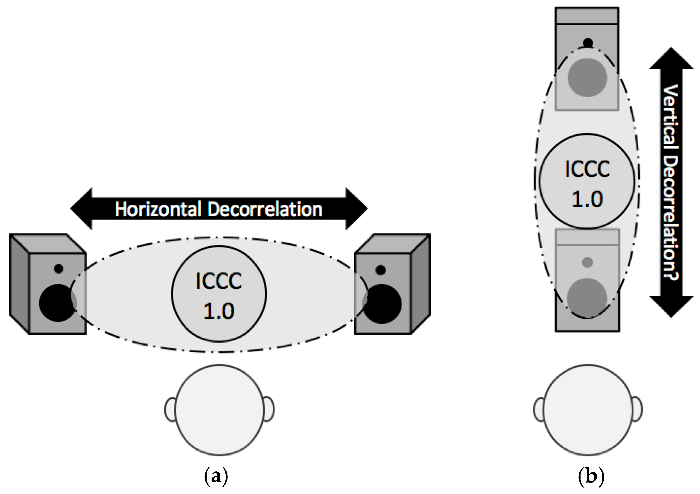
It is well documented in the literature that horizontal interchannel decorrelation between left and right loudspeaker signals relates directly to the perceived width of the horizontal auditory image [1]. This is due to a strong relationship between the interchannel cross-correlation (ICC) and interaural cross-correlation (IAC)—it is known that the IAC coefficient (IACC) is a good indicator of apparent source width (ASW) in concert hall acoustics, as dictated by decorrelated early reflections from lateral directions [2]. In turn, an artificial synthesis of this natural decorrelation controls the horizontal extent of a phantom auditory image between left and right loudspeaker channels. A visual representation of this can be seen on the left of Figure 1 below, where the phantom auditory image of the ICCC 1.0 condition (full correlation between the two loudspeaker signals) is narrow and located directly between the two source positions—decorrelation of the two signals then extends the horizontal image spread (HIS) towards the locations of the loudspeakers.
In contrast, very little is known about the psychoacoustic effects of interchannel decorrelation in the vertical domain. Research regarding vertical panning demonstrates that an elevated phantom image is generated between two spaced coherent signals (as represented by the ICCC 1.0 image on the right of Figure 1) [3,4,5]. However, there has been little investigation into how this phantom image is perceived when the correlation between the two signals is decreased. If the perception of vertical decorrelation were similar to that of horizontal decorrelation, then a decrease of correlation would result in an increase of vertical image spread (VIS) (as proposed in Figure 1), possibly mimicking the effect of decorrelated ceiling reflections—it has previously been suggested that a single ceiling reflection can increase the perception of VIS [6,7]. This comparison between horizontal and vertical decorrelation is the focus of the current experiment, where both domains are judged using the same stimuli and under the same testing conditions.
Taking into account the perceptual cues of vertical localisation, frequencies above around 3 kHz are important for elevation perception [8,9]; it could therefore be considered that any effect of vertical decorrelation might be frequency-dependent as well, potentially with a greater influence from the key high frequency regions related to vertical localisation. In order to observe the spectral impact alone, the current study assesses the effect of vertical decorrelation in the median plane where there is little interaural difference, except for that caused by ear asymmetry at high frequencies [10].
Considering the above background, the following research questions are proposed:
- Is there a direct relationship between vertical ICC and VIS in the median plane?
- How does vertical decorrelation compare to horizontal decorrelation?
- Is the perception of horizontal and vertical decorrelation frequency-dependent?
In order to answer the above questions, broadband pink noise has been filtered into three frequency bands: ‘Low’ (octave-bands with centre frequencies of 63–250 Hz), ‘Middle’ (centre frequencies of 0.5–2 kHz) and ‘High’ (centre frequencies of 4–16 kHz). These three frequency bands were each decorrelated with varying degrees of ICC and presented in multiple comparison trials (both horizontally and vertically), to observe whether an ICC effect is apparent for the different groups of frequencies. Two subjective listening tests were conducted to grade the perceived magnitudes of HIS and VIS for the stimuli with different frequency bands and ICCs. Preliminary results of the tests were presented in [11]. The current paper describes the experimental design in detail and provides complete statistical analyses of the data obtained. Furthermore, various objective measurements are carried out on the binaural recordings of the test stimuli in order to provide insights into potential cues that might have influenced the subjective results.
This paper is organised as follows. Experimental hypotheses are first presented in Section 2. Section 3 describes the experimental design. Following this, Section 4 and Section 5 detail the experimental results obtained on HIS and VIS, respectively. Section 6 provides discussion on the results of the two experiments with objective analysis of stimuli and room signals. Finally, Section 7 summarises and concludes the paper.
2. Experimental Hypotheses
Firstly, considering the horizontal part of the experiment, the accepted relationship between interchannel cross correlation (ICC), interaural cross-correlation (IAC) and the perceived horizontal image spread (HIS) has already been researched extensively [1]. Given this, it is hypothesised that decreasing the horizontal ICC between a pair of left and right loudspeakers will increase the perceived HIS (ASW), supporting the existing literature. In terms of frequency-dependency, previous research has demonstrated that the effect of IACC on the perception of ASW varies between different groups of frequencies [12]. In concert hall acoustics, an established measure of ASW involves calculating the average IACC of the 500 Hz, 1 kHz and 2 kHz octave-bands only (IACC3) [2]. These three bands were chosen as IACC appeared to align with changes to the absolute ASW angle for each—the 4 kHz octave-band also demonstrated a similar relationship, however, it was not included in the measure as musical signals have less relative energy at higher frequencies and there is little contribution to ASW above 3 kHz. Furthermore, lower frequencies are considered inherently broad and it is thought that decorrelation results in a relatively small change to the overall HIS by decorrelation, thus the low frequency exclusion from the IACC3 measure. From this, it is hypothesised that the greatest degree of HIS change by horizontal decorrelation will be observed for the ‘Middle’ frequency band (0.5–2 kHz octave-bands). The assessment of three separate frequency bands should provide novel insights of decorrelation perception, both horizontally and vertically.
Since previous studies have not formally assessed the effect of interchannel decorrelation in the vertical plane, a focus must be placed on existing vertical localisation and vertical panning literature. Research of vertical panning in the median plane indicates that two discrete coherent signals can be interpreted by the hearing system simultaneously, where an elevated phantom image is perceived between the two spaced positions [3,4,5]. As this level of cognition is well established, it is hypothesised that the hearing system is also able to perceive two partially correlated signals as a phantom image. Furthermore, partial correlation of two discrete signals from independent directions would imply that they emanate from a single source of great spatial extent, given the subtle phase and amplitude differences at arrival. It is further hypothesised that as correlation between the signals decreases, the two signal locations become more independent (yet remain sonically fused due to partial correlation), which in turn causes a relative increase to the perceived vertical image spread (VIS). Moreover, since vertical localisation and vertical panning are most effective for signals with higher frequency content (>~3 kHz) [5,8,9], it is also hypothesised that any effect of vertical decorrelation is likely to be strongest within this frequency region.
3. Experimental Design
3.1. Stimuli Creation
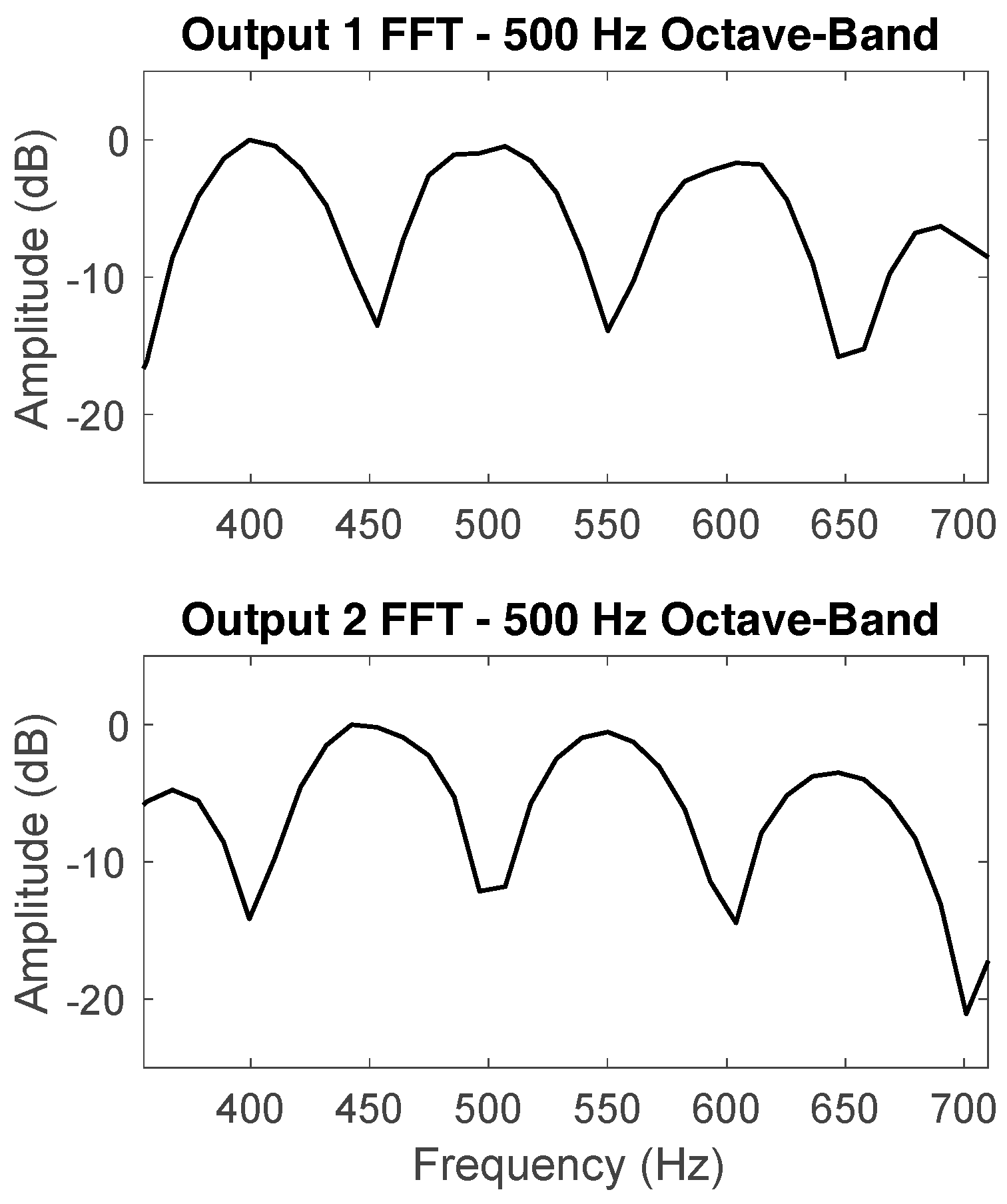
There are many approaches to achieve a decorrelation of signals—this is mostly through phase and/or spectral-amplitude alterations of an input signal to create two partially correlated output signals [1,13,14]. For the current experiments, the amplitude-based complementary comb-filtering method has been implemented, due to its advantages in computational efficiency and easy control over the degree of correlation between the output signals. First discovered by Lauridsen [14] and investigated further by Schroeder [15], the technique works on a basis of alternating frequency panning across the spectrum. It was found that summing and subtracting an input signal with a delayed version of itself creates a pair of comb-filtered signals with opposing amplitude differences—this is demonstrated in Figure 2, where the two outputs from the Lauridsen decorrelator are presented for a 500 Hz octave-band of pink noise. In Figure 2, the regular amplitude differences between the two channels are clearly seen, with Output 1 generated by summing a 10 ms delayed signal and Output 2 by subtracting a 10 ms delayed signal (described further below).
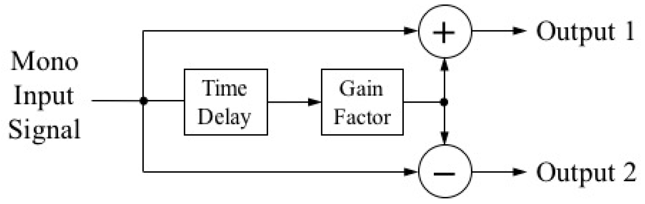
The regularity of these amplitude differences (i.e., the ‘tooth’ bandwidth) is dictated by the time-delay (T) of the secondary signal and a gain factor (G) applied to the delayed signal controls the notch depth and degree of decorrelation (between 0 and 1, where 1 is maximum decorrelation)—a block diagram of this process can be seen in Figure 3 below. Irwan and Aarts [16] used a time-delay of 10 ms in their proposed upmixing algorithm, which was determined experimentally as a compromise between adequate widening and avoiding confusion that can be experienced with longer time-delays. As far as the author is aware, there has been no formal assessment of the complementary comb-filtering parameters. It was thought that performing such an assessment within the context of the present experiment would provide a useful insight into the general perception of decorrelation, both horizontally and vertically. To this end, test stimuli were created with 1 ms, 5 ms, 10 ms and 20 ms time-delays for each frequency band; and to observe the effect of interchannel cross-correlation (ICC), the gain factor was set between 0.0 and 1.0 with increments of 0.2. This resulted in six stimuli being compared for each of the four time-delays within a particular frequency band—the six stimuli were judged in a multiple comparison format for each time-delay independently as described further in Section 3.4 below.
To assess the frequency-dependency of interchannel decorrelation, a continuous monophonic pink noise sample was filtered into three frequency bands using a brick-wall band-pass filter. Each frequency band spanned three octave-bands: ‘Low’ (octave-bands with centre frequencies of 64 Hz, 125 Hz and 250 Hz), ‘Middle’ (500 Hz, 1 kHz and 2 kHz) and ‘High’ (4 kHz, 8 kHz and 16 kHz). The Lauridsen decorrelation algorithm was implemented in MATLAB to process the three frequency bands, using the time-delay and gain factor settings described above. This resulted in a 12 multiple comparison trials for both the horizontal and vertical domains, made up of each frequency band and time-delay combination (3 × 4). During testing, all stimuli were level-matched and presented at an average un-weighted linear sound pressure level (SPL) of 72 dB(Z), producing a comfortable listening level for the subjects. Un-weighted SPL was used so that each frequency band would be presented at a similar level, avoiding the increase of energy for the low frequency band that would occur when level-matching SPL with A-weighting (dB(A)).
With the complementary comb-filtering method, predicted ICC coefficients (ICCCs) between the two output signals can be calculated using Equation (1) below, where ‘G’ is the gain factor [17]. The results for the gain factors used during the present investigation are displayed in Table 1 below. As expected, the calculated ICCC decreases as gain factor increases, providing the broad range of ICCC values required for the current experiment.
3.2. Physical Setup
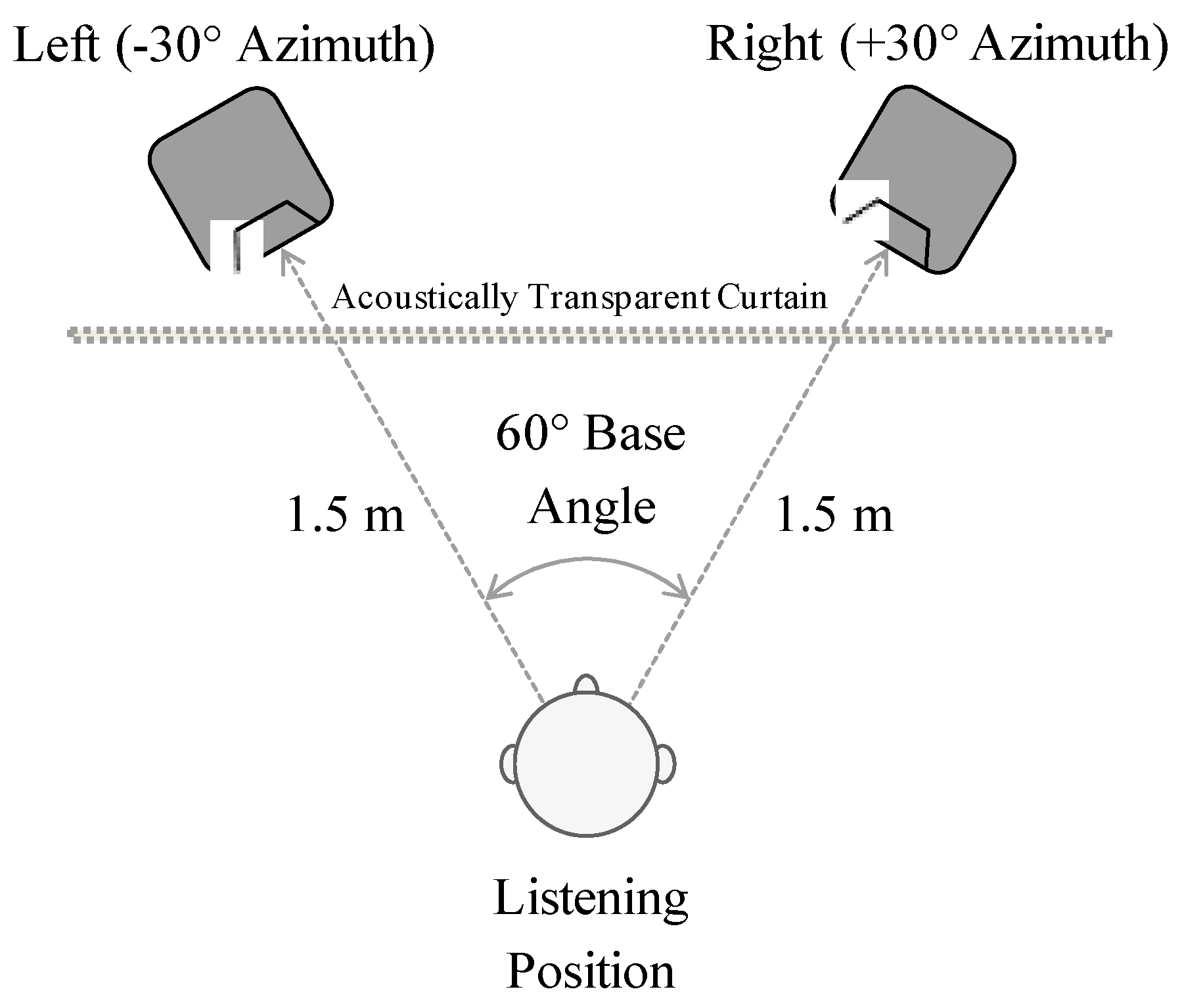
The listening tests were carried out in a semi-anechoic chamber at the University of Huddersfield, featuring a rubber floor and sound absorption on the walls and ceiling—further absorption was placed on the floor between the loudspeaker and listener to reduce the effect of floor reflections. All loudspeakers in both experimental parts were hidden from view by an acoustically transparent curtain, in order to conceal the test setup and avoid any visual bias that may occur. For the horizontal part, two Genelec 8040A loudspeakers (Frequency response: 48 Hz–20 kHz (±2 dB)) were positioned in the left and right stereophonic loudspeaker setup with a base angle of 60° (±30° azimuth), positioned at a distance of 1.5 m from the listener and 1.5 m from each other (see Figure 4). The listener was positioned at a height so that their ears were in line with the acoustic centre of both loudspeakers.
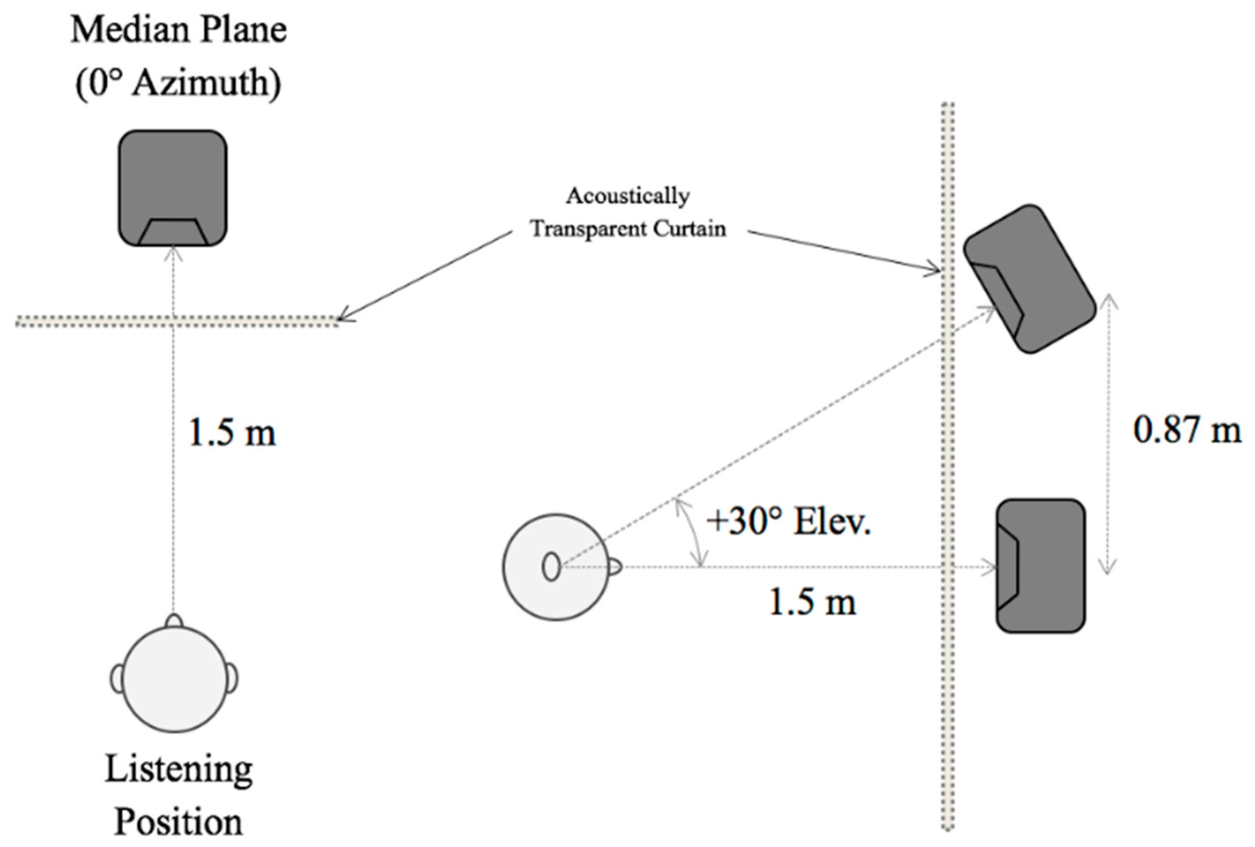
In the assessment of vertical decorrelation, two Genelec 8040A loudspeakers were vertically-arranged in the median plane, with the lower main-layer loudspeaker positioned 1.5 m in front of the listener and the upper height-layer loudspeaker elevated by +30° at a distance of 0.87 m directly above the lower loudspeaker (Figure 5). The two loudspeaker signals were time- and level-aligned at the listening position, to accommodate for a difference in distance from source to receiver. As with the horizontal test, loudspeakers were hidden by an acoustically transparent curtain and the listener was positioned so that their ears were in line with the acoustic centre of the lower loudspeaker.
3.3. Subject
The horizontal and vertical tests were carried out at separate times to ensure the testing conditions remained constant for each listener. As a result, not all subjects were available to sit both parts of the test. In total, 14 subjects took park in the horizontal test and 13 in the vertical test, with 10 subjects contributing to both. The subjects were trained listeners affiliated with the University of Huddersfield’s music technology courses—comprising staff members, final year undergraduate students and post-graduate research students—all of who were experienced with critical listening and analysis of spatial content in a listening test environment.
3.4. Test Method
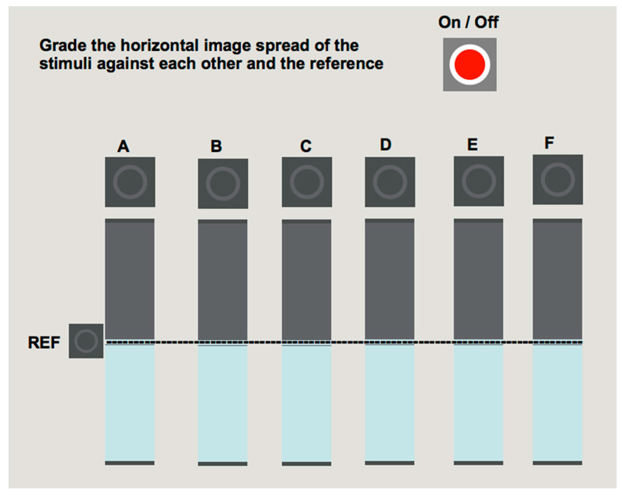
As previously mentioned, twelve multiple comparison trials were presented for both the horizontal and vertical conditions, made up of each time-delay and frequency band combination. Each multiple comparison trial featured 6 buttons and sliders to control and grade the 6 gain factor stimuli for a particular condition (with gain factors ranging from 0.0 to 1.0 at 0.2 increments). The multiple comparison test format was based on the MUSHRA standard in ITU-R BS.1534-3 [18]; however, rather than a scale of 0 to 100, a bi-polar scale was utilised ranging from −50 to 50, with a button for a reference stimulus positioned at 0 on the scale. The reference chosen was the ‘0.0’ gain factor condition of that particular trial, creating a hidden reference amongst the stimuli. In the case of the horizontal experiment, listeners were asked to grade the relative horizontal image spread (HIS) of each stimulus against each other and the reference; and with the vertical test, listeners were instructed to relatively grade vertical image spread (VIS). A bi-polar scale was used to avoid any grading bias, as it is not yet known whether decorrelation can cause the perception of VIS to decrease—unlike quality testing, it is impossible to provide a stimulus that has objectively the greatest or least amount of a spatial attribute. The testing interface was constructed in Cycling 74 Max 7 and can be seen in Figure 6—subjects could freely switch between stimuli and the reference throughout the test. The order of the presented stimuli and trials were randomised for each listener to reduce any psychological bias. Listeners were trained beforehand by being presented with an example of the grading interface and extreme stimuli (gain factors = 0.0 and 1.0), to familiarise them with the attribute(s) (HIS/VIS) and the format of testing.
4. Results and Analysis: Horizontal Decorrelation
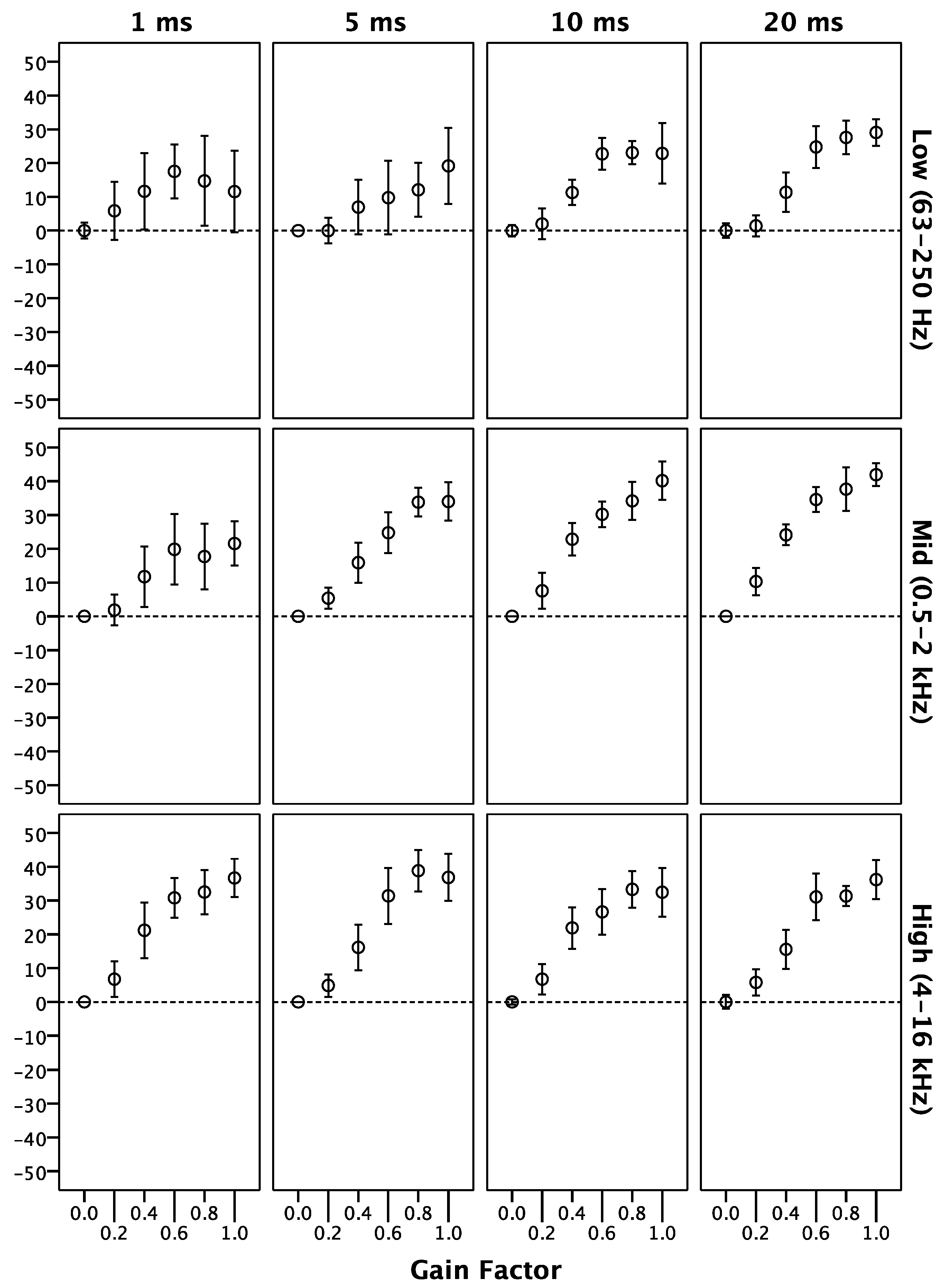
Results for the horizontal decorrelation test are presented in Figure 7—all data has been normalized in accordance with ITU-R BS.1116-3 [19] and analyzed in SPSS. The graphs display the median scores of relative horizontal image spread (HIS) with bars to signify notch edges, representing non-parametric 95% confidence intervals [20]. In order to determine whether the data fulfils the assumption of normality for parametric analysis, Shapiro-Wilk tests for normality were conducted on the data of each condition. The normality test results indicated that the data of each condition was not always normally distributed (violating the assumption); therefore, non-parametric statistical tests were performed across all conditions for consistency and comparison. Non-parametric Friedman repeated measure tests have been conducted on each frequency band and time-delay combination, in order to observe the main effect of gain factor (ICC) on HIS. Where a significant main effect is apparent, non-parametric Wilcoxon pairwise comparison tests have been carried out between each condition of that combination. Wilcoxon tests were used to determine whether a significant difference exists between two specific groups of data (i.e., a non-parametric equivalent of the ‘t-test’)—Bonferroni correction was then applied to the Wilcoxon results, so as to reduce the likelihood of a Type I error (incorrectly rejecting the null hypothesis).
Further to the tests described above, statistical correlation has also been calculated between gain factor and HIS for each condition, in order to observe the strength of the relationship between the two variables. The correlation results are presented in Table 2 below, where both Spearman’s rank-order and Pearson’s product-moment coefficients have been calculated. Spearman’s rank-order is non-parametric and observes a monotonic relationship, whereas Pearson’s product-moment determines the linearity of a relationship between two variables. Given that the data under analysis is not normally distributed, Spearman’s coefficients (rs) shall be referred to primarily; however, if agreement is seen with the respective Pearson coefficient (r), a linear relationship may also be suggested. Interpretation for both sets of correlation coefficients is as follows: 0.3–0.49 = weak, 0.5–0.69 = moderate, 0.7–0.89 = strong and 0.9–1.0 = very strong.
4.1. Low Frequency Band
The Friedman test results for the ‘Low’ frequency band (centre frequencies from 63 Hz to 250 Hz) show a significant gain factor effect on HIS for the 5 ms, 10 ms and 20 ms time-delays (p < 0.01) but not the 1 ms time-delay (p > 0.05). With the 5 ms time-delay, post-hoc Wilcoxon tests indicate there are no significant differences between conditions following Bonferroni correction. Wilcoxon tests with Bonferroni correction on the 10 ms data show significant differences between some conditions—gain factors of ‘0.6’, ‘0.8’ and ‘1.0’ had significantly greater HIS than the ‘0.0’ and ‘0.2’ gain factors; and a gain factor of ‘0.8’ was also significantly greater than ‘0.4’. For the 20 ms time-delay, the Bonferroni-corrected Wilcoxon results indicate that gain factors of ‘0.6’, ‘0.8’ and ‘1.0’ all had significantly greater HIS than the ‘0.0’, ‘0.2’ and ‘0.4’ gain factors. These results suggest that shorter time-delays are less effective at increasing HIS for lower frequencies, which is further reflected in the statistical correlation results of Table 2. It is seen that the statistical relationship between gain factor and HIS also increases as time-delay increases—10 ms has a moderate relationship between the two variables (rs = 0.65), while the correlation for a 20 ms time-delay is considered strong (rs = 0.82) (p < 0.01).
4.2. Middle Frequency Band
Friedman tests on the ‘Middle’ frequency band (centre frequencies from 0.5 kHz to 2 kHz) reveal a significant gain factor effect for all time-delays (p < 0.01). The 1 ms Wilcoxon results with Bonferroni correlation show that the gain factor of ‘1.0’ had a significantly greater HIS than the ‘0.0’ and ‘0.2’ gain factors (p < 0.05). With the 5 ms time-delay, the Wilcoxon results demonstrate that the gain factors of ‘0.6’, ‘0.8’ and ‘1.0’ were all significantly greater than the ‘0.0’, ‘0.2’ and ‘0.4’ gain factors (p < 0.05) but not each other (p > 0.05). For the 10 ms time-delay, all gain factor conditions were significantly greater than ‘0.0’ (p < 0.05); and ‘0.6’ and ‘0.8’ were also significantly greater than the ‘0.2’ and ‘0.4’ gain factors (p < 0.05). Lastly, the Wilcoxon results for a 20 ms time-delay show that gain factors of ‘0.4’, ‘0.6’, ‘0.8’ and ‘1.0’ all have a significant HIS increase over ‘0.0’ and ‘0.2’ gain factors; and gain factor ‘1.0’ is also significantly greater than ‘0.4’ and ‘0.6’ (p < 0.05). To support these results, the statistical correlation coefficients in Table 2 demonstrate that time-delays of 5 ms, 10 ms and 20 ms have a strong relationship between gain factor and HIS (rs > 0.7); on the other hand, the correlation for a 1 ms delay is only moderate (rs = 0.59) (p < 0.01), suggesting that longer time-delays are also more effective at middle frequencies, similar to that seen with the ‘Low’ frequency band. In general, the relationship between ICC and HIS appears to be particularly strong for the ‘Middle’ band, as was hypothesised at the beginning of the chapter.
4.3. High Frequency Band
The Freidman tests on the ‘High’ frequency band data (centre frequencies from 4 kHz to 16 kHz) show a significant gain factor effect for each of the time-delays (p < 0.01). Statistical correlation coefficients in Table 2 also indicate a strong relationship between gain factor and HIS for all time-delays (rs > 0.7) (p < 0.01). With the 1 ms delay, Bonferroni-corrected Wilcoxon results indicate that a gain factor of ‘1.0’ had significantly greater HIS than all other conditions (0.0–0.8) (p < 0.05); and ‘0.6’ and ‘0.8’ were also significantly greater than the ‘0.0’ and ‘0.2’ (p < 0.05). For 5 ms, ‘1.0’ and ‘0.8’ were significantly greater than ‘0.0’, ‘0.2’ and ‘0.4’ (p < 0.05). The 10 ms results show that a gain factors of ‘0.4’, ‘0.6’, ‘0.8’ and ‘1.0’ are all significantly greater than ‘0.0’ and ‘0.2’ gain factors (p < 0.05); and ‘0.8’ is also significantly greater than a gain factor of ‘0.4’ (p < 0.05). Finally, for the 20 ms time-delay, a gain factor of ‘1.0’ was significantly greater than the ‘0.0’, ‘0.2’, ‘0.4’ and ‘0.6’ gain factors (p < 0.05); and ‘0.6’ and ‘0.8’ were significantly greater than ‘0.0’, ‘0.2’ and ‘0.4’ (p < 0.05).
5. Results and Analysis: Vertical Decorrelation
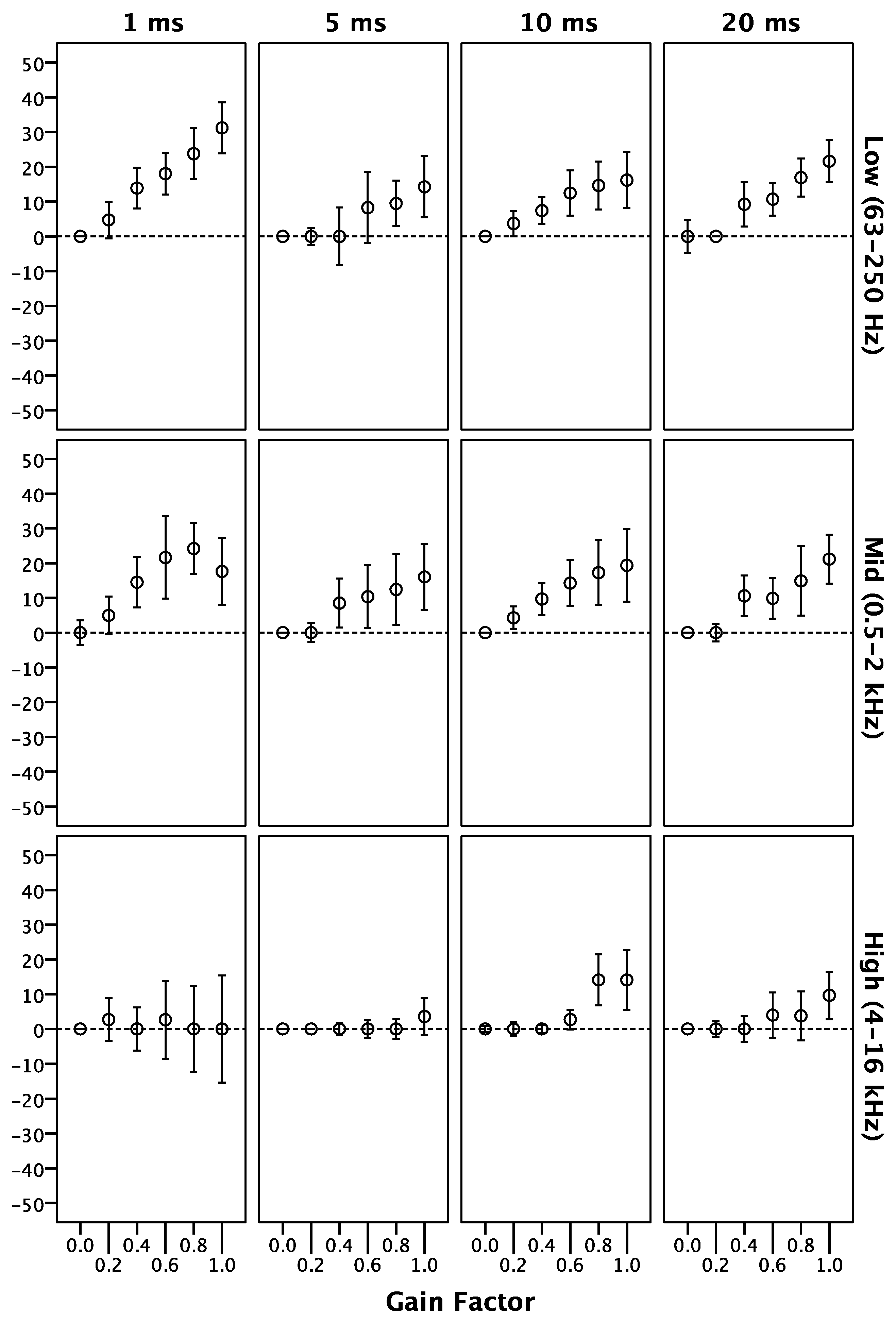
The results for the vertical decorrelation part of the experiment are presented in Figure 8, displaying the median and notch edge values (non-parametric 95% confidence equivalent). As with the HIS results, the relative vertical image spread (VIS) data was normalized in accordance with ITU-R BS.1116-3 [19] and analyzed in SPSS. Shapiro-Wilk tests of normality revealed that not all conditions had normally distributed data; as a result, non-parametric statistical tests were used to assess for significance within the data. The same statistical testing process was used as with the horizontal results (see Section 4), where Friedman tests were initially conducted to observe the gain factor effect within each time-delay and frequency band combination. Then, if a significant effect was detected, pairwise Wilcoxon tests with Bonferroni correction were performed between conditions to identify any significant difference. The statistical correlation results between gain factor and VIS for each condition are presented in Table 3 below, where both Spearman’s rank-order and Pearson’s product-moment coefficients have been calculated. As described above, Spearman’s test is non-parametric and looks at a monotonic relationship, whereas Pearson’s observes the linearity of correlation—both approaches can be interpreted as follows: 0.3–0.49 = weak, 0.5–0.69 = moderate, 0.7–0.89 = strong and 0.9–1.0 = very strong.
5.1. Low Frequency Band
Friedman tests of the ‘Low’ frequency band data (octave-band centre frequencies from 63 Hz to 250 Hz) reveal that all time-delays have a significant gain factor effect (p < 0.01). Post-hoc Wilcoxon tests with Bonferroni correction on the 1 ms data indicate that gain factors of ‘0.6’ and ‘1.0’ had significantly greater VIS than ‘0.0’ and ‘0.2’ (p < 0.05); furthermore, the ‘0.8’ gain factor was also significantly greater than ‘0.0’ (p < 0.05). For the 5 ms and 10 ms time-delays, the Wilcoxon tests show no significant difference between any conditions, following Bonferroni correction (p > 0.05). With the 20 ms delay, a gain factor of ‘0.8’ had significantly greater VIS than ‘0.2’ (p < 0.05). Furthermore, the statistical correlation results in Table 3 suggest that the relationship between gain factor and VIS is moderate for the 10 ms and 20 ms time-delays (rs = 0.58–0.63) but weaker for the 1ms and 5 ms delays (rs < 0.5) (p < 0.05).
5.2. Middle Frequency Band
The Friedman results for the ‘Middle’ frequency band (octave-band centre frequencies from 0.5 kHz to 2 kHz) show a significant gain factor effect for all time-delays (p > 0.05). The post-hoc Wilcoxon tests indicated no significant difference between gain factors for both the 1 ms and 5 ms delays, following Bonferroni correction (p > 0.05). On the other hand, with a 10 ms time-delay, gain factors of ‘0.4’, ‘0.6’ and ‘1.0’ had significantly greater VIS than ‘0.0’ and ‘0.2’ (p < 0.05); and for the 20 ms delay, a ‘1.0’ gain factor was perceived as significantly greater than ‘0.2’ (p < 0.05). The statistical correlation results in Table 3 indicate a moderate correlation between gain factor and VIS for the 20 ms time-delay (rs = 0.64), however, the relationship for the other time-delays is considered weak (rs < 0.5) (p < 0.01).
5.3. High Frequency Band
Results from the Friedman tests on the ‘High’ frequency band data (octave-band centre frequencies from 4 kHz to 16 kHz) reveal a significant gain factor effect for the 5 ms, 10 ms and 20 ms time-delays (p < 0.05) but not the 1 ms delay (p > 0.05). The Bonferroni-corrected Wilcoxon tests on the 5 ms and 20 ms data show no significant difference between any of the conditions (p > 0.05). However, the 10 ms Wilcoxon tests indicate a gain factor of ‘1.0’ produces a significantly greater VIS than the ‘0.0’ gain factor (p < 0.05). Furthermore, Table 3 indicates that the statistical correlation between gain factor and VIS is moderate for the 1 ms and 20 ms time-delays (rs = 0.59–0.62) but very weak for the 5 ms and 10 ms delays (rs < 0.3) (p < 0.01).
6. Discussion
Comparing both sets of results, there is a noticeable difference of relative spread perception between horizontal and vertical interchannel decorrelation. The horizontal results show that decorrelation is similarly effective at increasing horizontal image spread (HIS) for all frequency bands—however, a slightly longer time-delay is required for the ‘Low’ frequency band to generate significantly greater levels of HIS (this has been discussed further in Section 6.1 below). In contrast, vertical decorrelation in the median plane appears to be most effective for the ‘Low’ frequency band, though with little significant difference between conditions (unlike the results for horizontal decorrelation). The statistical correlation between gain factor and vertical image spread (VIS) is also noticeably lower for all vertical decorrelation conditions, in comparison to those for horizontal decorrelation. This suggests that, although significant changes to VIS by vertical decorrelation are observed in the median plane, the effect is weaker than that of horizontal decorrelation between a pair of left and right loudspeakers.
6.1. Interaural Cross-Correlation Coefficient (IACC)
Considering the relationship between horizontal decorrelation and interaural cross-correlation (IAC), Table 4 below displays the IAC coefficients (IACCs) of the binauralised stimuli signals in the horizontal plane. These results were calculated as the average IACC of 50 ms windows over time. For the binauralisation, a pair of head-related impulse responses (HRIRs) from the MIT KEMAR database [21] (left and right (±30°)) were convolved with the source signals of each condition. For the ‘Low’ and ‘High’ frequency bands, the results demonstrate that the IACC decreases as the gain factor increases (i.e., decreasing the ICCC)—this is the expected relationship between ICCC and IACC, as demonstrated in previous research [1]. However, for the ‘Middle’ frequency band, IACC appears to decrease up to a gain factor of 0.6, before slightly increasing as the gain increases further. The reason for this is not clear and the subjective results in Figure 7 do not seem to follow the same trend. Since Figure 7 shows that HIS increases as gain factor increases (ICCC decreases), the results in Table 4 suggest that IACC may not be a good predictor of HIS for middling frequencies—instead, calculation of ICCC may prove to be more accurate for HIS prediction in this region.
To investigate the IACC results for the ‘Middle’ band further, the binauralised ‘Middle’ stimuli have been filtered into the three contributing octave-bands (centre frequencies of 500 Hz, 1 kHz and 2 kHz), with Table 5 below displaying the 50 ms window averaged IACC for each octave-band filtered condition. Here the 500 Hz octave-band displays a decrease of IACC as the gain factor increases (i.e., ICCC decreases), corresponding with the subjective HIS results for the ‘Middle’ band in Figure 7. On the other hand, the 1 kHz band has a decrease of IACC up to a gain factor of ‘0.8’, which then increases again with a gain factor of ‘1.0’. Similarly, the 2 kHz band has a decrease of IACC up to ‘0.6’, followed by an increase of IACC as gain factor increases to ‘1.0’. This indicates that the IACC results seen in Table 4 are largely determined by the 1 kHz and 2 kHz octave-bands; however, if IACC does indeed contribute to HIS, it seems that the subjective results for the ‘Middle’ band may have been dictated by the 500 Hz octave-band. The apparent disagreement between the IACC results and subjective HIS results for the ‘Middle’ frequency band suggests that measurement of IACC in two-channel stereophony (with a base angle of 60°) may not be an accurate predictor of HIS, particularly for broader bands in the middle frequency region. It should also be said that the observed trend of IACC for the 1 kHz and 2 kHz octave-bands may be specific to the decorrelation method used in the present study; therefore, further investigations are required to observe the octave-band relationship between ICCC and IACC for different decorrelation techniques.
With regard to concert hall acoustics, the IACC3 measure considers that the greatest contributors of ASW lie within the frequencies of the ‘Middle’ band—it has been demonstrated concert hall studies that an increase of ASW corresponds with a decrease of IACC for the 500 Hz, 1 kHz and 2 kHz octave-bands [2]. The results in Table 4 and Table 5 appear to contradict with this somewhat, where only the IACCs of the 500 Hz octave-band correspond with the increasing trend seen in the subjective HIS results. As mentioned above, this effect may be specific to the decorrelation method used, however, it could also be an inherent limitation of IACC calculation when presenting audio in two-channel stereophony. In order to properly assess the use of IACC (or IACC3) for HIS prediction over loudspeakers, further investigation is required to compare ICCC, IACC and HIS at octave-band level, combined with the assessment of multiple decorrelation methods.
It is also interesting to note that significant increases of HIS were perceived for all three frequency bands in the subjective results, rather than just the ‘Middle’ band from which the IACC3 is measured. For the ‘Low’ band, it may be that these frequencies are mostly correlated in concert halls when summing at the ear, thus providing no contribution to the measurement of IACC; however, when two low frequency signals are artificially decorrelated between a left and right loudspeaker pair, the differences of interaural correlation would likely be greater, seemingly causing an increase of HIS. Moreover, high frequencies were not included in the IACC3 measure due to a lack of reflection energy at higher frequencies in concert halls—with that in mind, the results presented here strongly suggest that measuring the IACC of high frequencies can also contribute to the measurement of HIS in two-channel stereophony. A greater consideration of higher frequencies (4 kHz to 16 kHz octave-bands) could be the basis of accurate HIS measurement in surround sound reproduction, where high frequency energy may be considerably greater.
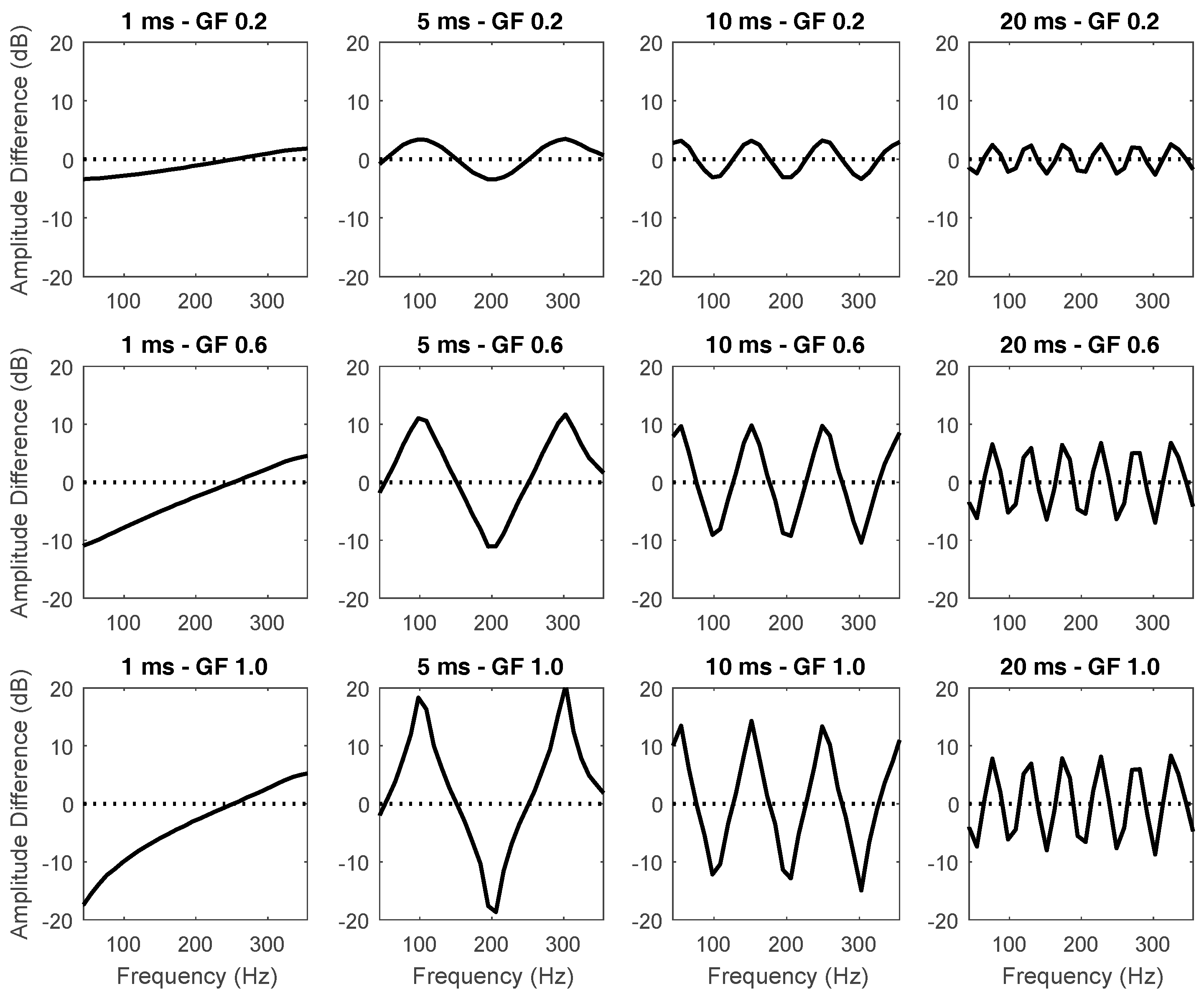
6.2. Low Frequency Band Discussion
In the subjective results, it is apparent that the perception of the ‘Low’ frequency band differs between horizontal and vertical decorrelation. In order to observe the effect of time-delay on the source signals for the ‘Low’ band, Figure 9 displays the difference of spectrum between the two output channels, with gain factors of ‘0.2’, ‘0.6’ and ‘1.0’ for each time-delay. Spectra were calculated as the long-term average FFT using 4096 FFT points and a frame size of 4096 samples (with 50% overlapping windows and no spectral smoothing). In the plots, a positive amplitude indicates a bias towards the right/height loudspeaker channel (for horizontal and vertical decorrelation, respectively), whereas a negative amplitude is a bias to the left/main loudspeaker channel.
From the Figure 9 plots, it can be seen that as time-delay decreases, the distribution of frequencies between the two channels becomes unbalanced. This is further reflected in Table 6, where the RMS of the two decorrelated output signals has been calculated for each time-delay, using a gain factor of ‘1.0’. With a 1 ms time-delay and gain factor of ‘1.0’, all frequencies below around 250 Hz are boosted in the left/main loudspeaker channel, resulting in a RMS difference between the two channels of 4.4 dB. In the case of horizontal decorrelation, this bias to the left loudspeaker may have caused the greater deviation of responses seen in the ‘Low’ frequency band subjective results (as suggested by the larger error bars for the 1 ms time-delay in Figure 7). Whereas for vertical decorrelation, the uneven frequency distribution with a 1 ms time-delay would have resulted in more energy in the lower main-layer loudspeaker below 250 Hz, potentially causing an increase of perceived loudness (despite SPL level-matching the conditions). It is hypothesised that such a change in perceived loudness could have caused the greater perception of VIS seen for the 1 ms time-delay in Figure 8, potentially from an enhanced floor reflection; having said that, the statistical correlation between gain factor and VIS for a 1 ms delay remains weak (rs = 0.42). These results suggest a 1 ms time-delay is unsuitable for decorrelating low frequency content. In future experimentation, it may also be useful to RMS level-match the two decorrelated outputs of the complementary comb-filtering method, in order to reduce a bias of energy towards one loudspeaker channel.
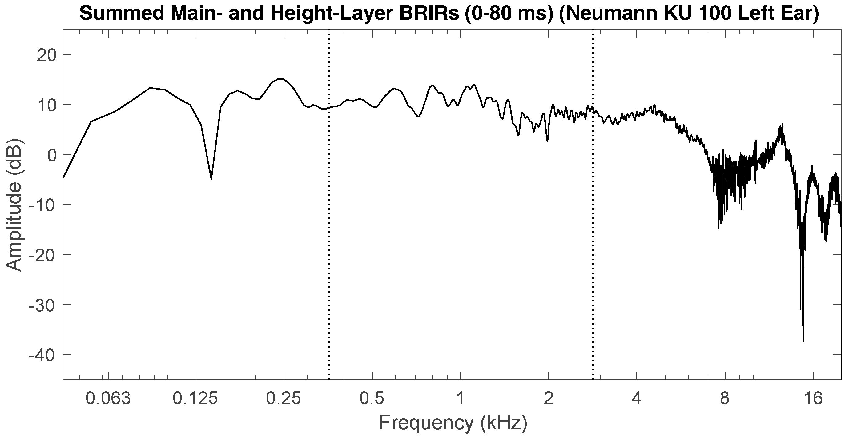
While uneven frequency distribution may account for the 1 ms vertical decorrelation results, VIS change was also seen for longer time-delays at low frequencies (though the differences were largely insignificant). As hypothesised above, a floor reflection may have influenced the perception of VIS, particularly when more energy is present in the lower main-layer loudspeaker. To look for a potential effect of the listening room on VIS perception, binaural room impulse responses (BRIRs) of the semi-anechoic chamber have been recorded using the HAART impulse response toolbox [22], which utilises the exponential sine sweep approach [23]. Sine sweeps were reproduced from both the main- and height-layer loudspeakers independently, with the signals captured by a Neumann KU100 dummy head located in the listening position. The main- and height-layer BRIRs were then time and level aligned, before being summed together to replicate the vertical testing condition.
Figure 10 displays the FFT of the summed BRIRs, calculated using 4096 FFT-points and a frame length of 4096 samples (with 50% overlapping hanning windows). On inspection of the spectrum, a large notch can be seen in the low frequency region around 140 Hz, as well as smaller notches in the ‘Middle’ frequency band (up to around 2 kHz). Given the regularity of the notches, it suggests a comb-filter effect due to a first reflection interacting with the direct sound—presumably from the rubber flooring of the semi-anechoic chamber (despite placing absorption on the floor between the listener and the loudspeakers). The first frequency notch of comb-filtering when two similar signals interact can be determined by Equation (2) below. The main-layer loudspeaker was located at 1.15 m above the ground and 1.5 m from the listening position—this results in a floor reflection path of around 1.25 m greater than the direct signal, with a delay of ~3.6 ms between their arrival at the ear. From this, it is calculated that the first comb-filter notch from a floor reflection should theoretically occur at 139 Hz—the similarity between this and the large notch observed in Figure 10 suggests that a floor reflection is indeed present. Previous research has shown that a single ceiling reflection can increase the perception of VIS [6,7]—further testing is required to observe whether a single floor reflection can also have a similar effect on the vertical image.
where is the time-delay between signals and is the first notch frequency of the comb-filter.
To analyse the summed main and height BRIRs further, the ratio of early reflection energy to direct sound energy (ER/D) at the listening position has been calculated using Equation (3) below. The results presented in Table 7 show that the ER/D is noticeably greater for the ‘Low’ frequency band (−1.9 dB) than the other bands (Table 7)—in other words, the floor reflection observed in Figure 10 is likely to have been heavily weighted with low frequency energy, while the higher frequencies were mostly absorbed. Hypothetically, a decorrelation of enhanced reflections might have led to a further increase of VIS with the ‘Low’ frequency band. If this were the case, it is possible that the results presented here are specific to the listening environment in which the testing was conducted. However, despite this, the subjective results still indicate that some change of VIS is perceivable at low frequencies, with further investigation required to ascertain the exact cause of the perception.
where is the impulse signal, is 0 ms, is 2.5 ms and is 80 ms.
6.3. High Frequency Band Discussion
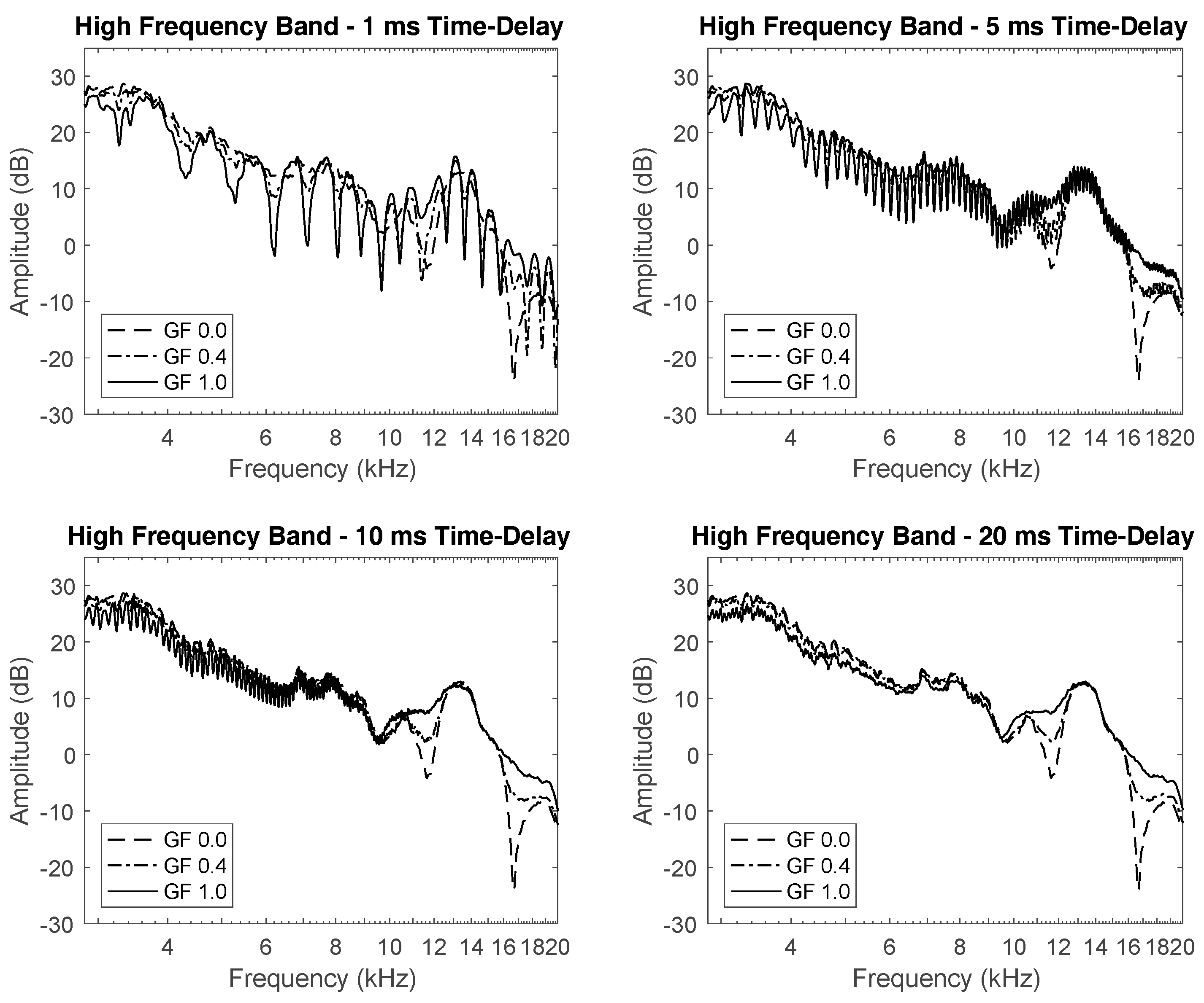
On further inspection of the vertically summed BRIR spectra in Figure 10, large notches can also be seen within the ‘High’ frequency band, specifically in the region of the 16 kHz octave-band—these notches are presumably due to HRTF filtering at the pinna [9]. To investigate the effect of the HRTF on the ‘High’ band, the vertical stimuli have been convolved with the sum of two anechoic head-related impulse responses (HRIRs) from MIT’s KEMAR dummy head database [21]—where one HRIR represents the main-layer loudspeaker angle (0° azimuth, 0° elevation) and the other the height-layer loudspeaker (0° azimuth, +30° elevation). In order to observe the gain factor effect on the ear input spectrum, the HRIR-convolved stimuli spectra have been plotted in Figure 11 for three gain factors (0.2, 0.4 and 1.0) of each time-delay—this is to demonstrate how the HRTF spectrum changes as the vertically-arranged signals are decorrelated, with only three gain factors plotted to improve clarity. The FFTs have been calculated as a long-term average using 4096 FFT-points and a frame length of 4096, with 1/96 octave spectral smoothing and 50% overlapping hanning windows.
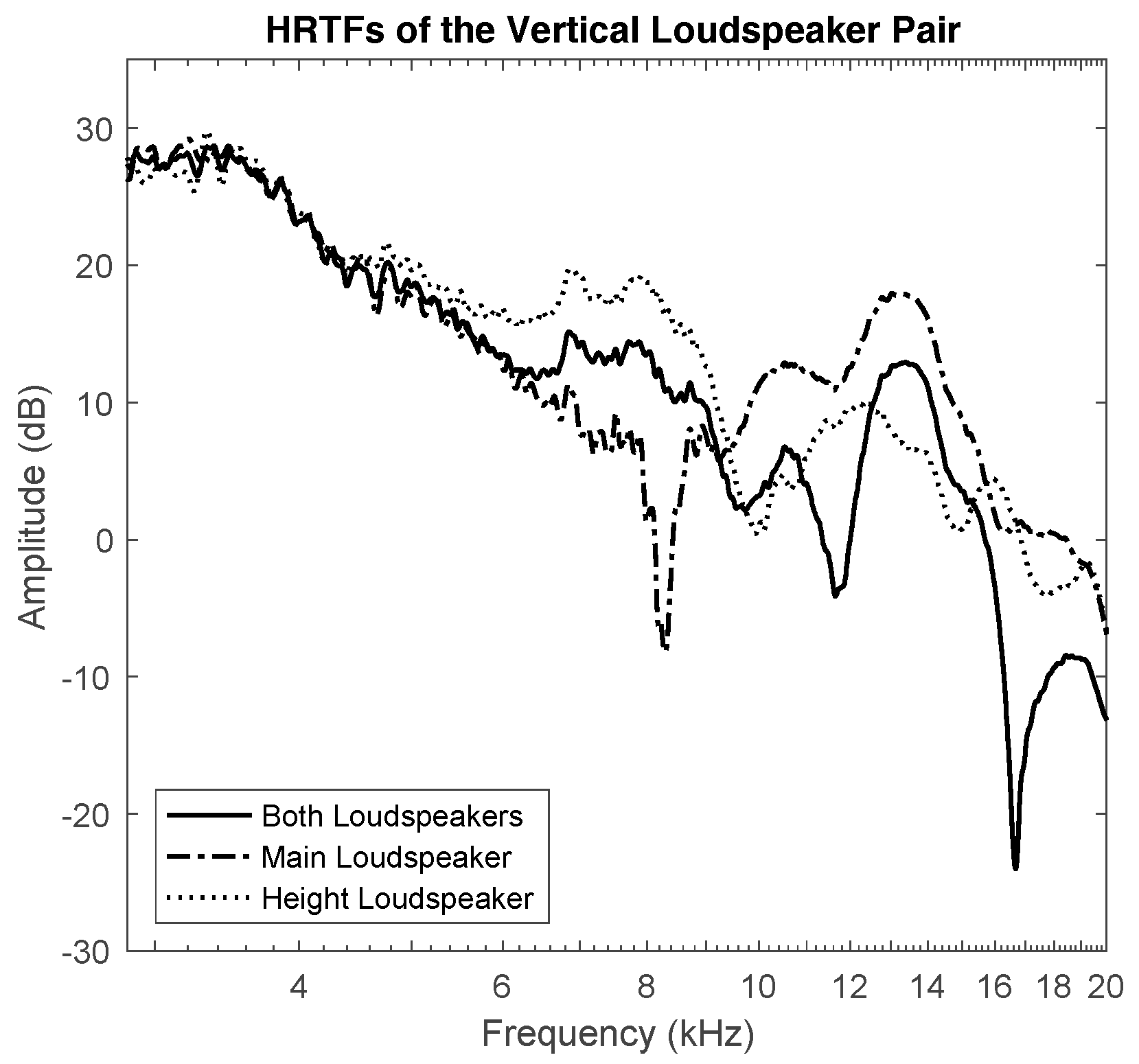
The spectra in Figure 11 display similar high frequency spectral notches to those observed in Figure 10—these notches are around 11.5 kHz and 17 kHz and appear to have the greatest depth when the signals are correlated (gain factor = 0.0). As the gain factor increases (i.e., as correlation between the main- and height-channels decreases), a spectral boost occurs in these regions and the notches become ‘filled in’. This is most apparent for the 10 ms and 20 ms time-delays, whereas with shorter delays, a comb-filtering effect occurs that noticeably distorts the definition of the notches. Furthermore, Figure 12 below compares the HRTFs for each loudspeaker position independently against the HRTF for the loudspeakers combined (i.e., the vertical stereophonic test condition). Here it is seen that the notches displayed in the plots of Figure 11 appear to be unrelated to the individual main- and height-layer loudspeaker HRTFs, which suggests that these notches are specific to the vertical stereophonic condition.
From these observations, it is hypothesised that the filling in notches provides a spectral cue for the perception of VIS; however, further investigations are required to explore whether this is indeed the case. If the spectral notches (and subsequent filling from decorrelation) are an important cue for VIS perception, the increase of spectral distortion with shorter time-delays would inevitably have an impact on the detection of such cues. This is reflected in the vertical decorrelation subjective results (Figure 8), where larger error bars are seen for the 1 ms time-delay and a significant gain factor effect is only apparent for the 5 ms time-delay and above—the only significant difference between individual gain factor conditions for the ‘High’ band was seen with a time-delay of 10 ms.
Despite clear spectral changes in the ‘High’ frequency band as correlation decreases, little significant change of VIS is seen between the different gain factor conditions in the subjective results (Figure 8). One possibility is that this could be related to the un-weighted sound pressure level (SPL) (dB(Z)) used during testing, which is likely to produce differences in loudness between the frequency bands. It is known from the literature that presentation level has an impact on the perceived extent of a source, where a greater level increases the size of an auditory event [24]. To quantify the loudness of each band, Table 8 displays the LUFS (LKFS) values [25] for the correlated stimuli source signals used during testing, as calculated by Adobe Audition. The results show a +4 dB increase of loudness for the ‘High’ frequency band compared to the ‘Low’ frequency band (when both have been SPL level-matched). Table 8 also displays the LUFS values calculated for a pink noise signal that has been filtered into the same frequency bands used during testing. Pink noise has equal energy for each octave-band and is thought to roughly represent the typical octave-band relationship within a complex signal. Looking at Table 8, the pink noise LUFS results demonstrate that the relative loudness of the ‘High’ frequency band is considerably lower than that of the ‘Low’ frequency band. When comparing this against the LUFS of the test stimuli, it is clear that the levels used during testing are not representative of a typical interband frequency relationship found in a complex source. Given that the loudness of the high frequency stimuli was comparatively high during testing, it may have resulted in an increased perception of VIS for all conditions, resulting in more subtle VIS changes from decorrelation—further testing on this hypothesis is required to determine the effect of level and loudness on VIS perception.
The loudness level of the ‘High’ frequency band stimuli signal (Table 8) could also be related to a lack of reflective energy at high frequencies. As seen with the ER/D in Table 7, the ‘Low’ frequency band has the greatest amount of early reflective energy, suggesting that less amplification would be required to meet the target SPL. In contrast, given the greater absorption at high frequencies in the semi-anechoic chamber, it is thought that the ‘High’ frequency band would require more amplification at line level to match the same SPL.
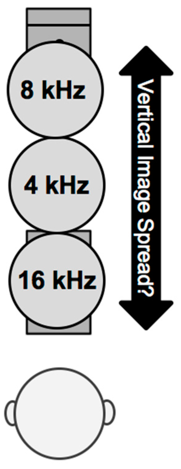
Another reason for a lack of significant VIS difference between the ‘High’ frequency band conditions in the subjective testing could be related to the “pitch-height effect” [24,26,27] and “directional bands effect” [28,29]. From the directional band research, it is known that 4 kHz and 16 kHz bands tend to be perceived in front and an 8 kHz band is often perceived above (if presented under anechoic conditions). Similarly, when octave-band noise signals are presented at ear height from in front of the listener, a “pitch-height effect” occurs which sees the 8 kHz octave-band elevated upwards (towards the position of the height-channel loudspeaker); whereas the 16 kHz band is localised towards the main-channel loudspeaker and 4 kHz is perceived somewhere between the two [24,26]. Wallis and Lee [27] have demonstrated that this effect also occurs when coherent octave-bands are presented in vertical stereophony, i.e., the same signal reproduced in a main-layer loudspeaker and a height-layer loudspeaker simultaneously (both of which are located in the median plane, similar to the test condition in the current experiment). It is hypothesised that this natural vertical spread of frequencies may also be apparent in the ‘High’ frequency band signals, resulting in an initial broad VIS when both signals are correlated (gain factor = 0.0), with relatively small changes to VIS from decorrelation as the gain factor increases. The potential perception of this has been illustrated in Figure 13, showing the possible distribution of octave-bands across the frontal vertical image. To investigate this hypothesis further, it would be useful to conduct experiments on the absolute extent of VIS for individual octave-bands, as well as for broadband signals—results from such an investigation would give important insights into the inherent perception of VIS by vertical interchannel decorrelation.
7. Conclusions
Two listening tests have been conducted to observe the effects of interchannel decorrelation both horizontally and vertically. Decorrelated stimuli were generated using the complementary comb-filtering decorrelation method, where frequencies are alternately distributed between two channels throughout the spectrum. The decorrelation method is controlled by two variables: time-delay and gain factor. Time-delay determines the bandwidth between the comb-filter notches and the gain factor defines the notch depth, which in turn controls the degree of decorrelation (between 0.0 and 1.0, where 1.0 is maximum decorrelation). Variations of these variables were assessed during testing, with time-delays of 1 ms, 5 ms, 10 ms and 20 ms and six gain factors from 0.0 to 1.0 at increments of 0.2. These conditions were applied to three frequency bands: ‘Low’ (octave-bands with centre frequencies of 63 Hz, 125 Hz and 250 Hz), ‘Middle’ (centre frequencies of 0.5 kHz, 1 kHz and 2 kHz) and ‘High’ (centre frequencies of 4 kHz, 8 kHz and 16 kHz).
For the horizontal decorrelation, the two decorrelated signals were routed to left and right loudspeakers, respectively, with a base angle of 60° (±30° azimuth). During the horizontal test, subjects were asked to grade the relative horizontal image spread (HIS) between the different gain factor stimuli within each time-delay. With the vertical decorrelation test, signals were decorrelated in the median plane (0° azimuth), between a main-layer loudspeaker positioned at ear height (0° elevation) and another positioned directly above at an elevation of +30°—subjects were asked to grade the vertical image spread (VIS) between stimuli.
The key findings from the listening tests are as follows:
- A significant effect of interchannel decorrelation on auditory image spread is apparent both horizontally and vertically, where phantom image spread increases as correlation decreases.
- The decorrelation effect appears to be stronger in the horizontal domain, with moderate-strong statistical correlation between gain factor and HIS for all frequency bands.
- Vertical decorrelation also leads to significant increases of VIS, however, the relationship between gain factor and VIS appears to be weaker.
- The results also suggest that the perception of vertical decorrelation is frequency-dependent, with VIS change most apparent in the ‘Low’ frequency band.
- Perception of vertical decorrelation for the ‘Low’ and ‘Middle’ frequency bands could potentially be related to floor reflections within the listening room.
- Vertical decorrelation of the ‘High’ frequency band appears to be associated with spectral notches, which may act as cues for the perception of VIS.
- The interaural cross-correlation coefficient (IACC) appears to be a good predictor of horizontal spread in most cases, however, some disagreement is seen for the ‘Middle’ band.
- A time-delay of 1 ms causes an uneven distribution of frequency energy in the ‘Low’ frequency band, making it unsuitable for low frequency band-limited decorrelation.
The above findings suggest that vertical interchannel decorrelation has some influence on the perception of VIS in the median plane. However, further investigation is required to reveal the extent of those changes, as well as any frequency or presentation angle dependency on VIS perception.
Acknowledgments
This work was supported by the Engineering and Physical Sciences Research Council (EPSRC), UK, Grant Ref. EP/L019906/1. The authors would like to thank the staff members and students of the University of Huddersfield’s music technology courses who took part in the listening tests.
Author Contributions
Christopher Gribben conducted the experiment, analyzed the data and wrote the paper. Hyunkook Lee supervised the work and contributed to the data analysis and discussion presented in the paper.
Conflicts of Interest
The authors declare no conflict of interest.
References
- Zotter, F.; Frank, M. Efficient Phantom Source Widening. Arch. Acoust. 2013, 38, 27–37. [Google Scholar] [CrossRef]
- Hidaka, T.; Beranek, L.L.; Okano, T. Interaural cross-correlation (IACC), lateral fraction (LF) and low- and high-frequency sound levels (G) as measures of acoustical quality in concert halls. J. Acoust. Soc. Am. 2013, 97, 3319. [Google Scholar] [CrossRef]
- Pulkki, V. Localization of Amplitude-Panned Virtual Sources II: Two- and Three-Dimensional Panning. J. Audio Eng. Soc. 2001, 49, 753–767. [Google Scholar]
- Barbour, J.L. Elevation perception: Phantom images in the vertical hemi-sphere. In Proceedings of the Audio Engineering Society 24th International Conference on Multichannel Audio: The New Reality, Banff, AB, Canada, 26–28 June 2003. [Google Scholar]
- Mironovs, M.; Lee, H. The Influence of Source Spectrum and Loudspeaker Azimuth on Vertical Amplitude Panning. In Proceedings of the 142nd Convention of the Audio Engineering Society, Berlin, Germany, 20–23 May 2017. [Google Scholar]
- Furuya, H.; Fujimoto, K.; Takeshima, Y.; Nakamura, H. Effect of Early Reflections from Upside on Auditory Envelopment. J. Acoust. Soc. Jpn. 1995, 16, 97–104. [Google Scholar] [CrossRef]
- Robotham, R.; Stephenson, M.; Lee, H. The Effect of a Vertical Reflection on the Relationship between Preference and Perceived Change in Timbral and Spatial Attributes. In Proceedings of the 140th Convention of the Audio Engineering Society, Paris, France, 4–7 June 2016. [Google Scholar]
- Roffler, S.K.; Butler, R.A. Factors that Influence the Localization of Sound in the Vertical Plane. J. Acoust. Soc. Am. 1968, 43, 1255–1259. [Google Scholar] [CrossRef] [PubMed]
- Hebrank, J.; Wright, D. Spectral Cues used in the Localization of Sound Sources on the Median Plane. J. Acoust. Soc. Am. 1974, 56, 1829–1834. [Google Scholar] [CrossRef] [PubMed]
- Carlile, S.; Pralong, D. Location-Dependent Nature of Perceptually Salient Features of the Human Head-Related Transfer Functions. J. Acoust. Soc. Am. 1994, 95, 3445–3459. [Google Scholar] [CrossRef]
- Gribben, C.; Lee, H. The Perceptual Effects of Horizontal and Vertical Interchannel Decorrelation, using the Lauridsen Decorrelator. In Proceedings of the 136th Convention of the Audio Engineering Society, Berlin, Germany, 26–29 April 2014. [Google Scholar]
- Mason, R.; Brookes, T.; Rumsey, F. Frequency Dependency of the Relationship between Perceived Auditory Source Width and the Interaural Cross-Correlation Coefficient for Time-Invariant Stimuli. J. Acoust. Soc. Am. 2005, 117, 1337–1350. [Google Scholar] [CrossRef] [PubMed] [Green Version]
- Kendall, G.S. The Decorrelation of Audio Signals and its Impact on Spatial Imagery. Comput. Music J. 1995, 19, 71–87. [Google Scholar] [CrossRef]
- Lauridsen, H. Nogle Forsøg Reed Forskellige Former Rum Akustik Gengivelse. Ingeniøren 1954, 47, 906–910. [Google Scholar]
- Schroeder, M.R. An Artificial Stereophonic Effect Obtained from a Single Audio Source. J. Audio Eng. Soc. 1958, 6, 74–79. [Google Scholar]
- Irwan, R.; Aarts, R.M. Two-to-Five Channel Sound Processing. J. Audio Eng. Soc. 2002, 50, 914–926. [Google Scholar]
- Breebart, J.; Faller, C. Spatial Audio Processing: MPEG Surround and Other Applications; John Wiley: Chichester, UK, 2007. [Google Scholar]
- International Telecommunications Union (ITU-R). Recommendation ITU-R BS.1534-3: Method for the Subjective Assessment of Intermediate Quality Level of Audio Systems, International Telecommunications Union: Geneva, Switzerland, 2015.
- International Telecommunications Union (ITU-R). Recommendation ITU-R BS.1116-3: Methods for the Subjective Assessment of Small Impairments in Audio Systems; International Telecommunications Union: Geneva, Switzerland, 2015. [Google Scholar]
- McGill, R.; Tukey, J.W.; Larsen, W.A. Variations of Box Plots. Am. Stat. 1978, 32, 12–16. [Google Scholar]
- Gardner, B.; Martin, K. HRTF Measurements of a Kemar Dummy-Head Microphone. In MIT Media Lab Perceptual Computing; Technical Report #280; MIT Media Lab: Cambridge, MA, USA, 1994. [Google Scholar]
- Johnson, D.; Harker, A.; Lee, H. HAART: A New Impulse Response Toolbox for Spatial Audio Research. In Proceedings of the 138th Convention of the Audio Engineering Society, Warsaw, Poland, 7–10 May 2015. [Google Scholar]
- Farina, A. Simultaneous Measurement of Impulse Response and Distortion with a Swept-Sine Technique. In Proceedings of the 110th Convention of the Audio Engineering Society, Amsterdam, The Netherlands, 12–15 May 2000. [Google Scholar]
- Cabrera, D.; Tilley, S. Vertical Localization and Image Size Effects in Loudspeaker Reproduction. In Proceedings of the Audio Engineering Society 24th International Conference: Multichannel Audio—The New Reality, Banff, AB, Canada, 26–28 June 2003. [Google Scholar]
- ITU-R. Recommendation ITU-R BS.1770-4: Algorithms to Measure Audio Programme Loudness and True-Peak Audio Level; International Telecommunications Union: Geneva, Switzerland, 2015. [Google Scholar]
- Lee, H. Perceptual Band Allocation (PBA) for the Rendering of Vertical Image Spread with a Vertical 2D Loudspeaker Array. J. Audio Eng. Soc. 2016, 64, 1003–1013. [Google Scholar] [CrossRef]
- Wallis, R.; Lee, H. The Effect of Interchannel Time Difference on Localization in Vertical Stereophony. J. Audio Eng. Soc. 2015, 63, 767–776. [Google Scholar] [CrossRef]
- Blauert, J. Sound Localization in the Median Plane. Acustica 1969, 22, 205–213. [Google Scholar]
- Wallis, R.; Lee, H. Directional Bands Revisited. In Proceedings of the 138th Convention of the Audio Engineering Society, Warsaw, Poland, 7–10 May 2015. [Google Scholar]
Figure 1.
Visualisation of horizontal and (potential) vertical interchannel decorrelation perception. ICCC 1.0 is full correlation between the two loudspeaker signals, producing a narrow auditory phantom image. (a) Horizontal Image Spread (HIS); (b) Potential Vertical Image Spread (VIS).
Figure 1.
Visualisation of horizontal and (potential) vertical interchannel decorrelation perception. ICCC 1.0 is full correlation between the two loudspeaker signals, producing a narrow auditory phantom image. (a) Horizontal Image Spread (HIS); (b) Potential Vertical Image Spread (VIS).

Figure 2.
FFT plots of the Complementary Comb-Filtered output signals (500 Hz octave-band with a 10 ms time-delay and gain factor of 1.0).
Figure 2.
FFT plots of the Complementary Comb-Filtered output signals (500 Hz octave-band with a 10 ms time-delay and gain factor of 1.0).

Figure 3.
Structure of the Complementary Comb-Filtering decorrelator [17].
Figure 3.
Structure of the Complementary Comb-Filtering decorrelator [17].

Figure 4.
Horizontal loudspeaker setup with a 60° base angle.

Figure 5.
Vertical loudspeaker setup at 0° azimuth with a +30° elevation.

Figure 6.
Multiple comparison interface used during testing, constructed in Max 7.

Figure 7.
Results of the relative horizontal image spread (HIS) by interchannel decorrelation. Median values and notch edges (95% confidence).
Figure 7.
Results of the relative horizontal image spread (HIS) by interchannel decorrelation. Median values and notch edges (95% confidence).

Figure 8.
Results of the relative vertical image spread (VIS) by interchannel decorrelation. Median values and notch edges (95% confidence).
Figure 8.
Results of the relative vertical image spread (VIS) by interchannel decorrelation. Median values and notch edges (95% confidence).

Figure 9.
Delta spectra between the output signals for the ‘Low’ frequency band i.e., the interchannel level difference (ICLD): ‘S2–S1’, where S1 is the left/main source signal and S2 is the right/height source signal.
Figure 9.
Delta spectra between the output signals for the ‘Low’ frequency band i.e., the interchannel level difference (ICLD): ‘S2–S1’, where S1 is the left/main source signal and S2 is the right/height source signal.

Figure 10.
FFT of the summed main- and height-layer BRIRs (0–80 ms) from the semi-anechoic chamber. The vertical dotted lines signify the cut-off frequency between the frequency bands.
Figure 10.
FFT of the summed main- and height-layer BRIRs (0–80 ms) from the semi-anechoic chamber. The vertical dotted lines signify the cut-off frequency between the frequency bands.

Figure 11.
FFTs of HRIR-convolved stimuli for the vertical decorrelation conditions. Gain factors of 0.0, 0.4 and 1.0 are plotted for each time-delay.
Figure 11.
FFTs of HRIR-convolved stimuli for the vertical decorrelation conditions. Gain factors of 0.0, 0.4 and 1.0 are plotted for each time-delay.

Figure 12.
FFTs of the HRTFs from the lower main-layer loudspeaker, the upper height-layer loudspeaker and both of the loudspeakers combined (i.e., the vertical stereophonic test condition).
Figure 12.
FFTs of the HRTFs from the lower main-layer loudspeaker, the upper height-layer loudspeaker and both of the loudspeakers combined (i.e., the vertical stereophonic test condition).

Figure 13.
Possible perception of vertical image spread (VIS) for the ‘High’ frequency band, based on the “pitch-height effect” phenomenon [24,26,27].


Table 1.
Calculated interchannel cross-correlation coefficients (ICCCs) for the complementary comb filter gain factors used during testing (based on Equation (1)).
Table 1.
Calculated interchannel cross-correlation coefficients (ICCCs) for the complementary comb filter gain factors used during testing (based on Equation (1)).
| Gain Factor (G) | 0.0 | 0.2 | 0.4 | 0.6 | 0.8 | 1.0 |
| ICCC | 1.00 | 0.92 | 0.72 | 0.47 | 0.22 | 0.00 |
Table 2.
Statistical Correlation between the gain factor of the complementary comb-filtering method and the relative Horizontal Image Spread (HIS) Scores (** p < 0.01; * p < 0.05).
Table 2.
Statistical Correlation between the gain factor of the complementary comb-filtering method and the relative Horizontal Image Spread (HIS) Scores (** p < 0.01; * p < 0.05).
| Spearman’s Rank-Order (rs) | Pearson’s Product-Moment (r) | |||||||
|---|---|---|---|---|---|---|---|---|
| Frequency Band | 1 ms | 5 ms | 10 ms | 20 ms | 1 ms | 5 ms | 10 ms | 20 ms |
| Low (63–250 Hz) | 0.27 * | 0.46 ** | 0.65 ** | 0.82 ** | 0.25 * | 0.40 ** | 0.65 ** | 0.83 ** |
| Middle (0.5–2 kHz) | 0.59 ** | 0.88 ** | 0.80 ** | 0.88 ** | 0.55 ** | 0.87 ** | 0.81 ** | 0.88 ** |
| High (4–16 kHz) | 0.80 ** | 0.81 ** | 0.78 ** | 0.85 ** | 0.80 ** | 0.81 ** | 0.78 ** | 0.86 ** |
Table 3.
Statistical Correlation between the gain factor of the complementary comb-filtering method and the relative Vertical Image Spread (VIS) Scores (** p < 0.01; * p < 0.05).
Table 3.
Statistical Correlation between the gain factor of the complementary comb-filtering method and the relative Vertical Image Spread (VIS) Scores (** p < 0.01; * p < 0.05).
| Spearman’s Rank-Order (rs) | Pearson’s Product-Moment (r) | |||||||
|---|---|---|---|---|---|---|---|---|
| Frequency Band | 1 ms | 5 ms | 10 ms | 20 ms | 1 ms | 5 ms | 10 ms | 20 ms |
| Low (63–250 Hz) | 0.42 ** | 0.49 ** | 0.63 ** | 0.58 ** | 0.45 ** | 0.45 ** | 0.66 ** | 0.57 ** |
| Middle (0.5–2 kHz) | 0.41 ** | 0.13 | 0.34 ** | 0.64 ** | 0.39 ** | 0.16 | 0.31 ** | 0.63 ** |
| High (4–16 kHz) | 0.59 ** | 0.06 | 0.29 ** | 0.62 * | 0.54 ** | 0.02 | 0.22 * | 0.63 * |
Table 4.
Interaural cross-correlation coefficients (IACCs) of the binauralised complementary comb-filter decorrelated stimuli (calculated as the average of 50 ms windows over time).
Table 4.
Interaural cross-correlation coefficients (IACCs) of the binauralised complementary comb-filter decorrelated stimuli (calculated as the average of 50 ms windows over time).
| Time-Delay (TD) | Gain Factor (G) | ||||||
|---|---|---|---|---|---|---|---|
| 0.0 | 0.2 | 0.4 | 0.6 | 0.8 | 1.0 | ||
| Low | 1 ms | 1.00 | 1.00 | 0.99 | 0.99 | 0.97 | 0.96 |
| 5 ms | 1.00 | 0.99 | 0.98 | 0.95 | 0.91 | 0.86 | |
| 10 ms | 1.00 | 0.99 | 0.98 | 0.95 | 0.91 | 0.86 | |
| 20 ms | 1.00 | 0.99 | 0.98 | 0.95 | 0.91 | 0.86 | |
| Middle | 1 ms | 1.00 | 0.79 | 0.54 | 0.46 | 0.45 | 0.55 |
| 5 ms | 1.00 | 0.78 | 0.35 | 0.21 | 0.36 | 0.52 | |
| 10 ms | 1.00 | 0.78 | 0.35 | 0.21 | 0.35 | 0.51 | |
| 20 ms | 1.00 | 0.78 | 0.35 | 0.22 | 0.36 | 0.51 | |
| High | 1 ms | 1.00 | 0.96 | 0.84 | 0.67 | 0.50 | 0.41 |
| 5 ms | 1.00 | 0.96 | 0.84 | 0.67 | 0.48 | 0.35 | |
| 10 ms | 1.00 | 0.96 | 0.84 | 0.67 | 0.48 | 0.34 | |
| 20 ms | 1.00 | 0.96 | 0.84 | 0.67 | 0.48 | 0.34 | |
Table 5.
Interaural cross-correlation coefficients (IACCs) of the octave-band filtered ‘Middle’ decorrelated stimuli (calculated as the average of 50 ms windows over time).
Table 5.
Interaural cross-correlation coefficients (IACCs) of the octave-band filtered ‘Middle’ decorrelated stimuli (calculated as the average of 50 ms windows over time).
| Time-Delay (TD) | Gain Factor (G) | ||||||
|---|---|---|---|---|---|---|---|
| 0.0 | 0.2 | 0.4 | 0.6 | 0.8 | 1.0 | ||
| 500 Hz | 1 ms | 1.00 | 0.98 | 0.91 | 0.82 | 0.74 | 0.67 |
| 5 ms | 1.00 | 0.96 | 0.84 | 0.67 | 0.49 | 0.34 | |
| 10 ms | 1.00 | 0.96 | 0.83 | 0.67 | 0.49 | 0.33 | |
| 20 ms | 1.00 | 0.96 | 0.83 | 0.66 | 0.49 | 0.33 | |
| 1 kHz | 1 ms | 1.00 | 0.89 | 0.76 | 0.62 | 0.53 | 0.59 |
| 5 ms | 1.00 | 0.87 | 0.58 | 0.28 | 0.17 | 0.30 | |
| 10 ms | 1.00 | 0.87 | 0.58 | 0.28 | 0.18 | 0.30 | |
| 20 ms | 1.00 | 0.87 | 0.58 | 0.29 | 0.19 | 0.30 | |
| 2 kHz | 1 ms | 1.00 | 0.79 | 0.59 | 0.52 | 0.49 | 0.60 |
| 5 ms | 1.00 | 0.76 | 0.31 | 0.21 | 0.40 | 0.56 | |
| 10 ms | 1.00 | 0.76 | 0.32 | 0.21 | 0.40 | 0.56 | |
| 20 ms | 1.00 | 0.76 | 0.32 | 0.23 | 0.40 | 0.56 | |
Table 6.
RMS of the two output channels for the ‘Low’ frequency band with a gain factor of 1.0.
| Left/Main Channel | Right/Height Channel | |
|---|---|---|
| 1 ms | −5.8 dB | −10.3 dB |
| 5 ms | −7.2 dB | −7.9 dB |
| 10 ms | −7.4 dB | −7.6 dB |
| 20 ms | −7.5 dB | −7.5 dB |
Table 7.
Early Reflection Energy (2.5–80 ms) to Direct Sound Energy (0–2.5 ms) Ratio (ER/D) for the summed main- and height-layer BRIRs.
Table 7.
Early Reflection Energy (2.5–80 ms) to Direct Sound Energy (0–2.5 ms) Ratio (ER/D) for the summed main- and height-layer BRIRs.
| Low Frequency Band | Middle Frequency Band | High Frequency Band |
|---|---|---|
| −1.9 dB | −14.2 dB | −17.3 dB |
Table 8.
A comparison of loudness level (LUFS) between the correlated stimuli used during testing (gain factor = 0.0) and pink noise filtered into the three frequency bands.
Table 8.
A comparison of loudness level (LUFS) between the correlated stimuli used during testing (gain factor = 0.0) and pink noise filtered into the three frequency bands.
| Low Frequency Band | Mid. Frequency Band | High Frequency Band | |
|---|---|---|---|
| Test Stimuli Signals | −16 dB LUFS | −14 dB LUFS | −12 dB LUFS |
| Filtered Pink Noise | −16 dB LUFS | −22 dB LUFS | −27 dB LUFS |
© 2017 by the authors. Licensee MDPI, Basel, Switzerland. This article is an open access article distributed under the terms and conditions of the Creative Commons Attribution (CC BY) license (http://creativecommons.org/licenses/by/4.0/).
Share and Cite
MDPI and ACS Style
Gribben, C.; Lee, H. A Comparison between Horizontal and Vertical Interchannel Decorrelation. Appl. Sci. 2017, 7, 1202. https://0-doi-org.brum.beds.ac.uk/10.3390/app7111202
AMA Style
Gribben C, Lee H. A Comparison between Horizontal and Vertical Interchannel Decorrelation. Applied Sciences. 2017; 7(11):1202. https://0-doi-org.brum.beds.ac.uk/10.3390/app7111202
Chicago/Turabian StyleGribben, Christopher, and Hyunkook Lee. 2017. "A Comparison between Horizontal and Vertical Interchannel Decorrelation" Applied Sciences 7, no. 11: 1202. https://0-doi-org.brum.beds.ac.uk/10.3390/app7111202
Note that from the first issue of 2016, this journal uses article numbers instead of page numbers. See further details here.