
EigenScape: A Database of Spatial Acoustic Scene Recordings


Audio Lab, Department of Electronic Engineering, University of York, Heslington, York YO10 5DQ, UK
*
Author to whom correspondence should be addressed.
Appl. Sci. 2017, 7(11), 1204; https://0-doi-org.brum.beds.ac.uk/10.3390/app7111204
Submission received: 23 October 2017
/
Revised: 21 November 2017
/
Accepted: 8 November 2017
/
Published: 22 November 2017
(This article belongs to the Special Issue Sound and Music Computing)
Abstract
:The classification of acoustic scenes and events is an emerging area of research in the field of machine listening. Most of the research conducted so far uses spectral features extracted from monaural or stereophonic audio rather than spatial features extracted from multichannel recordings. This is partly due to the lack thus far of a substantial body of spatial recordings of acoustic scenes. This paper formally introduces EigenScape, a new database of fourth-order Ambisonic recordings of eight different acoustic scene classes. The potential applications of a spatial machine listening system are discussed before detailed information on the recording process and dataset are provided. A baseline spatial classification system using directional audio coding (DirAC) techniques is detailed and results from this classifier are presented. The classifier is shown to give good overall scene classification accuracy across the dataset, with 7 of 8 scenes being classified with an accuracy of greater than 60% with an 11% improvement in overall accuracy compared to use of Mel-frequency cepstral coefficient (MFCC) features. Further analysis of the results shows potential improvements to the classifier. It is concluded that the results validate the new database and show that spatial features can characterise acoustic scenes and as such are worthy of further investigation.
1. Introduction
Since machine listening became an eminent field in the early 1990s, the vast majority of research has focused on automatic speech recognition (ASR) [1] and computational solutions to the well-known ‘cocktail party problem’—the “ability to listen to and follow one speaker in the presence of others” [2]. This is now a mature field of study, with robust speech recognition systems featured in most modern smartphones. There has also been a great deal of research on music information retrieval (MIR) [3], a technology with applications in intelligent playlist algorithms used by online music streaming services [4]. There has been comparatively little research investigating the automatic recognition of general acoustic scenes or acoustic events, though there has been an increase in interest in this area in recent years, largely due to the annual Detection and Classification of Acoustic Scenes and Events (DCASE) challenges established in 2013 [5].
The DCASE challenges have attracted a large number of submissions designed to solve the problem of acoustic scene classification (ASC) or acoustic event detection (AED). A typical ASC or AED system requires a feature extraction stage in order to reduce the complexity of the data to be classified. The key is the coarsening of the available data such that similar sounds will yield similar features (generalisation), yet the features should be distinguishable from those yielded by different types of sounds (discrimination). Generally, the audio is split into frames and some kind of mathematical transform is applied in order to extract a feature vector from each frame. Features extracted from labelled recordings (training data) are used to train some form of classification algorithm, which can then be used to return labels for new unlabelled recordings (testing data). See [6] for a thorough overview of this process.
The systems submitted to DCASE all identify acoustic scenes and events based upon features extracted from monaural or stereophonic recordings. A small number of systems have used spatial features extracted from binaural recordings [7,8,9], but the potential for extracting features using more sophisticated spatial recordings remains almost completely unexplored. This is due to a number of factors, including inheritance of techniques from ASR and MIR and the envisioned applications of ASC and AED.
A majority of the early research into ASR approached the problem with the aim of emulating elements of human sound perception. This “biologically relevant” [1] approach can be seen in the popular Mel-frequency cepstral coefficient (MFCC) features, which use a mel-scaled filter bank in order to crudely emulate the human cochlear response [10]. A more fundamental self-imposed limitation of this approach is the use of one- or two-microphone recordings. Although, on introducing the DCASE challenge, Stowell et al. stated that “human-centric aims do not directly reflect our goal... which is to develop systems that can extract semantic information about the environment around them from audio data” [5], it is natural to inherit techniques from more mature related fields.
The most commonly stated applications of ASC and AED technologies include adding context-awareness to smart devices, wearable technology, or robotics [6] where mounting of spatial microphone arrays would perhaps be more impractical. Another application is automatic labelling of archive audio, where the majority of recordings will be in mono or stereo format [5,6].
Some lesser-considered applications of ASC and AED technology involve the holistic analysis of acoustic scenes in and of themselves. The focus here is gaining a greater understanding of the constituent parts of acoustic scenes and how they change over time. This has potential applications in acoustic ecology research for natural environments, re-synthesis of acoustic scenes for virtual reality, and in obtaining more detailed measures for urban environmental sound than the prevailing sound level metric. The measurement aggregates all sound present in a scene into one single sound level figure. This disregards the variety of sources of the sounds, influencing much environmental sound legislation to focus on its suppression—an “environmental noise approach” [11]. A machine listening system could consider the content of an acoustic scene as well as absolute sound levels. This information could be used to create more subtle metrics regarding urban sound, taking into account human perception and preference—a “soundscape approach” [11]. This kind of system was proposed by Bunting et al. [12], but despite some promising work involving source separation in Ambisonic audio [13], published results from that project have been limited. The term soundscape is used here according to the ISO definition, meaning “the acoustic environment of a place, as perceived by people, whose character is the result of the action and interaction of natural and/or human factors” [14]. This emphasis on perception is apt in this case, but a subjective perceptual construct is clearly not what a machine listening system will receive as input for analysis. We therefore use the term ‘acoustic scene’ when discussing recordings.
Another potential application of such a system is assisting in the synthesis of acoustic scenes for experimental purposes. If a researcher or organisation wishes to obtain detailed data on human perception of environmental sound, one technique that can be used is a sound walk, in which listening tests can be conducted in situ at a location of interest. This gives the most realistic stimulus possible, direct from the environment itself. Results gained using this technique are therefore as representative as possible of subjects’ reactions with respect to the real-world acoustic environment, a factor known as ‘ecological validity’ [15,16]. The key disadvantages are that this method is not repeatable [15] and can be very time-consuming [17]. An alternative is laboratory reproduction of acoustic scenes, presented either binaurally [18] or using Ambisonics [19,20]. These are less time-consuming and more repeatable [15], but the clear disadvantage is the potential for reduced ecological validity of the results, which leads to the criticism that lab results “ought to be validated in situ” [21]. A key issue is how to condense an urban sound recording into a shorter format whilst retaining ecological validity. Methods for this have included selection of small clips at random [15] or manually arranging a acoustic scene “composition” in order to “create a balanced impression” [19]—essentially condensing the acoustic scene by ear. Whilst manual composition of a stimulus is undoubtably more robust than presentation of a random short clip that may or may not be representative of the acoustic scene as a whole, it is not an optimal process. The subjective recomposition of an acoustic scene by a researcher introduces a source of bias that could be reflected in the results. A machine listening system could effectively bypass this issue by providing detailed analysis that could assist with synthesis of shorter clips that remained statistically representative of real acoustic scenes.
The limitation to low channel counts is less applicable given these applications of machine listening technology. Spatial recordings offer the potential for a rich new source of information that could be utilised by machine listening systems and higher channel counts offer the opportunity for sophisticated source separation [13,22] which could assist with event detection.
The lack of research into classification using spatial audio features could also be due to the fact that there has been, as yet, no comprehensive database of spatially-recorded acoustic scenes. Any modern database of recordings intended for use in ASC research must contain many examples of each location class. This is to avoid the situation whereby classification results are artificially exaggerated due to test clips being extracted from the same longer recordings as clips used to train classifiers, as exemplified in [23].
A similar phenomenon has been seen in MIR research where classifiers were tested on tracks from the same albums as their training material [24]. The TUT Database [25], used in DCASE challenges since 2016, fulfils this criterion. It features recordings of 15 different acoustic scene classes made across a wide variety of locations, with details provided in order to avoid any crossover in locations between the training and testing sets. This database was recorded using binaural in-ear microphones. The DCASE 2013 AED task [5] used a small set of office recordings made in Ambisonic B-format (though only stereo versions were released as part of the challenge). Since it was intended for AED, this dataset features recordings of office environments only, not the wide range of locations needed for ASC work. The DEMAND database [26] features spatial recordings of six different acoustic scene classes, each recorded over three different locations. This is a substantial amount of data, but potentially still too small a collection for effective classifier training and validation. The recordings were made using a custom-made 16-channel microphone grid, which offers potential for spatial information extraction, though techniques developed using this data might not be generalisable to other microphone setups. This paper introduces EigenScape, a database of fourth-order Ambisonic recordings of a variety of urban and natural acoustic scenes for research into acoustic scene and event detection. The database and associated materials are freely available—see Supplementary Materials for the relevant URLs.
The paper is organised as follows: Section 2 covers the technical details of the recording process, provides information on the recorded data itself, and describes the baseline classification used for initial analysis of the database. Section 3 gives detailed results from the baseline classifier and offers some analysis of its behaviour and the implications this has for the dataset. Section 4 offers some additional discussion of the results, details potential further work, and concludes the paper.
2. Materials and Methods
2.1. Recording
EigenScape was recorded using the mh Acoustics EigenMike [27], a 32-channel spherical microphone array capable of recording up to fourth-order Ambisonic format. In Bates’ Ambisonic microphone comparisons [28,29] the EigenMike is among the lowest rated in terms of perceptual audio quality, rated as sounding “dull” compared to other microphones. Conversely, directional analysis shows the EigenMike gives the highest directional accuracy of any of the microphones tested, including the popular first-order Ambisonic Soundfield MKV and Core Sound TetraMic. It should be noted that the analysis in [28,29] used only the first-order output from the EigenMike (for parity with the other microphones), disregarding the higher-order channels. Since the dataset presented in this paper is primarily aimed at machine (rather than human) listening, and the EigenMike can record far more detailed spatial information than first-order microphones whilst retaining a relatively portable form factor, the EigenMike was chosen for this task.
Recordings were made using the proprietary EigenMike Microphone Interface Box and EigenStudio recording application [27]. Recordings were made at 24-bit/48 kHz resolution and the files use Ambisonic Channel Number (ACN) ordering [30]. All the recordings used a gain level of +25 dB set within the EigenStudio software as the ambient sound at many recording locations did not yield an adequate recording level at lower gain levels. The only exception to this is the recording labelled ‘TrainStation-08’, which used only +5 dB gain as very high level locomotive engine noise present at that location caused severe clipping at +25 dB.
For the majority of the recordings, the EigenMike was mounted in a Rycote windshield designed for use with the SoundField ST350 microphone [31]. Although the windshield was not designed for the EigenMike, care was taken to rigidly mount the microphone and the shield was effective in cancelling wind noise. The first few recordings used a custom-made windshield, but this was switched for the Rycote as the set-up time proved far too long. One indoor recording did not use any windshield. The discrepancies in windshield use and gain level should be negligible by comparison to the wide variety of sounds present in the scenes, especially when coarse features are extracted for use in a machine listening system. Such a system should be robust to the small spectral changes incurred by use of different windshields and to differences in ambient sound level between scenes. Indeed, the DARES project [32] used entirely different recording setups for indoor and outdoor recordings and this was judged to have “minimal influence on the quality of the database”. Nevertheless, these discrepancies are noted in metadata provided for EigenScape.
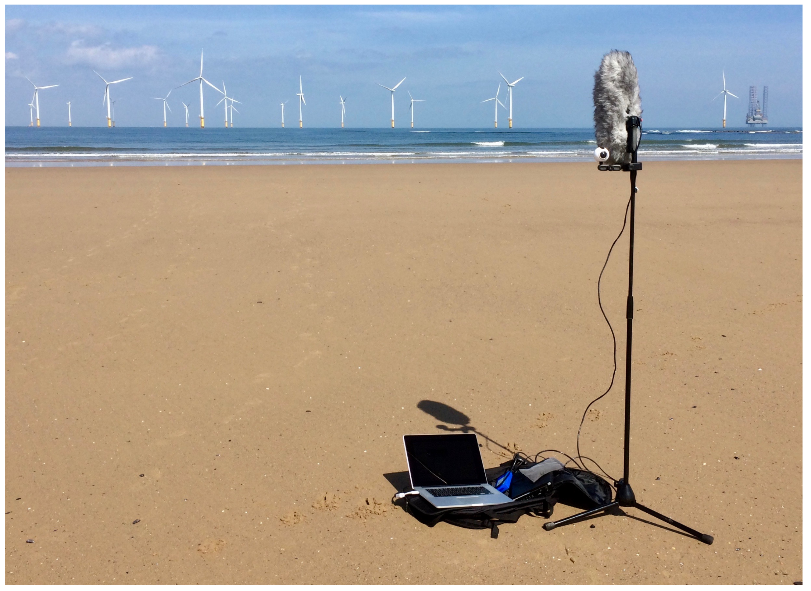
To make these recordings, the microphone was mounted on a standard microphone stand set to around head height. A Samsung Gear 360 camera [33] was also mounted to the tripod, recording video in order to assist with future annotation of events within scenes where the sound might be ambiguous. Figure 1 shows the full recording apparatus.
2.2. Details
Eight different examples each of eight different classes of acoustic scene were recorded for a total of 64 recordings. All recordings are exactly 10 minutes in length. The uniform recording duration facilitates easy segmentation into clips of equal length (e.g., 20 segments, each 30 s long). Basic segmentation tools are available with the dataset in order to assist with this. The recordings were planned out specifically to create a completely evenly-weighted dataset between the various scenes and to facilitate easy partitioning into folds (e.g., six recordings used for training, the other two used for testing).
The location classes were inspired by the classes featured in the TUT database: lakeside beach, bus, cafe/restaurant, car, city center, forest path, grocery store, home, library, metro station, office, urban park, residential area, train, and tram [25], but restricted to open public spaces, reflecting the shifted focus of this work towards acoustic scene analysis. The eight classes in EigenScape are as follows: Beach, Busy Street, Park, Pedestrian Zone, Quiet Street, Shopping Centre, Train Station, and Woodland. These location classes were chosen to give a good variety of acoustic environments found in urban areas and to be relatively accessible for the recording process. The recordings were made at locations across the North of England in May 2017. An online map has been created showing all the recording sites and is listed in Supplementary Materials. Basic location details are included in the dataset metadata, along with recording dates and times. Although individual consent is not required for recording in public spaces, permissions of the relevant local authorities or premises management was sought where possible. Some locations would not allow tripod-based recordings, so the microphone stand was held as a monopod. These are noted in the metadata.
A little over 10 minutes was recorded at each location, with a short amount of time removed from the beginning and end of each file post-recording. This removed the experimenter noise incurred by activating and deactivating the equipment and achieved the exactly uniform length of the audio clips. During recording, every effort was made to minimise sound introduced to the scene by the experimenter or equipment. It should be noted that occasionally a curious passerby would ask about what was happening. This was fairly unavoidable in busier public places, but since conversation is part of the acoustic scenes of such locations, these incidents should not affect feature extraction too much. Discretion is advised if these recordings are used for listening tests or as background ambiences in sound design work.
The complete dataset has been made available online for download. The full database is presented in uncompressed WAV format within a series of ZIP files organised by class. Since each recording is 10 minutes of 25 tracks at 24-bit/48 kHz, the whole set is just under 140 GB in size. As this could potentially be very taxing on disk space and problematic to download on slower internet connections, a second version of the dataset was created for easier access. This second version consists of all the recordings, but limited to the first-order Ambisonic channels (four tracks) and losslessly compressed to FLAC format within a single ZIP file. This results in a much more manageable size of 12.6 GB, whilst still enabling spatial audio analysis and reproduction. This is also in accordance with the UK Data Service’s recommended format for audio data [34].
2.3. Baseline Classification
To create a baseline for this database that utilises spatial information whilst maintaining a level of parity with the MFCC-Gaussian mixture model (GMM) baseline typically used in DCASE challenges [5,6,25], the audio was filtered into 20 mel-spaced frequency bands (covering the frequency range up to 12 kHz) using a bank of bandpass finite impulse response (FIR) filters. The filters each used 2048 taps and were designed using hamming windows. Estimate direction of arrival (DOA) estimates to be used as features were extracted from each band using directional audio coding (DirAC) analysis [35,36,37] as follows:
where contains the 20 mel-filtered versions of the zeroth-order Ambisonic channel (W) of the recording and contains the filtered versions of the first-order Ambisonic bi-directional X, Y and Z-channels in a three-dimensional matrix. Resultant matrix contains instantaneous DOA estimates for each frequency band. Mean values of were calculated over a frame length of 2048 samples, with 25% overlap between frames. Angular values for azimuth and elevation were derived from this as follows [38]:
where , , and are the X, Y and Z channel matrices extracted from . These angular values were used as features. Diffuseness values were also used as features, and were calculated as follows [36]:
where {.} represents the mean-per-frame values described previously, c is the speed of sound, and:
where is the characteristic acoustic impedance and is the mean density of air.
The database was split into four folds for cross-validation. In each fold, six location class recordings were used for training, with the remaining two used for testing. The extracted DirAC features from each frame of the training audio were used to train a bank of 10-component GMMs (one per scene class). The test audio was cut into 30-s segments (40 segments in total for testing). Features were extracted from these segments, and each GMM gave a probability score for the frames. These scores were summed across frames from the entire 30-s segment, with the segment classified according to the model which gave the highest total probability score across all frames.
3. Results
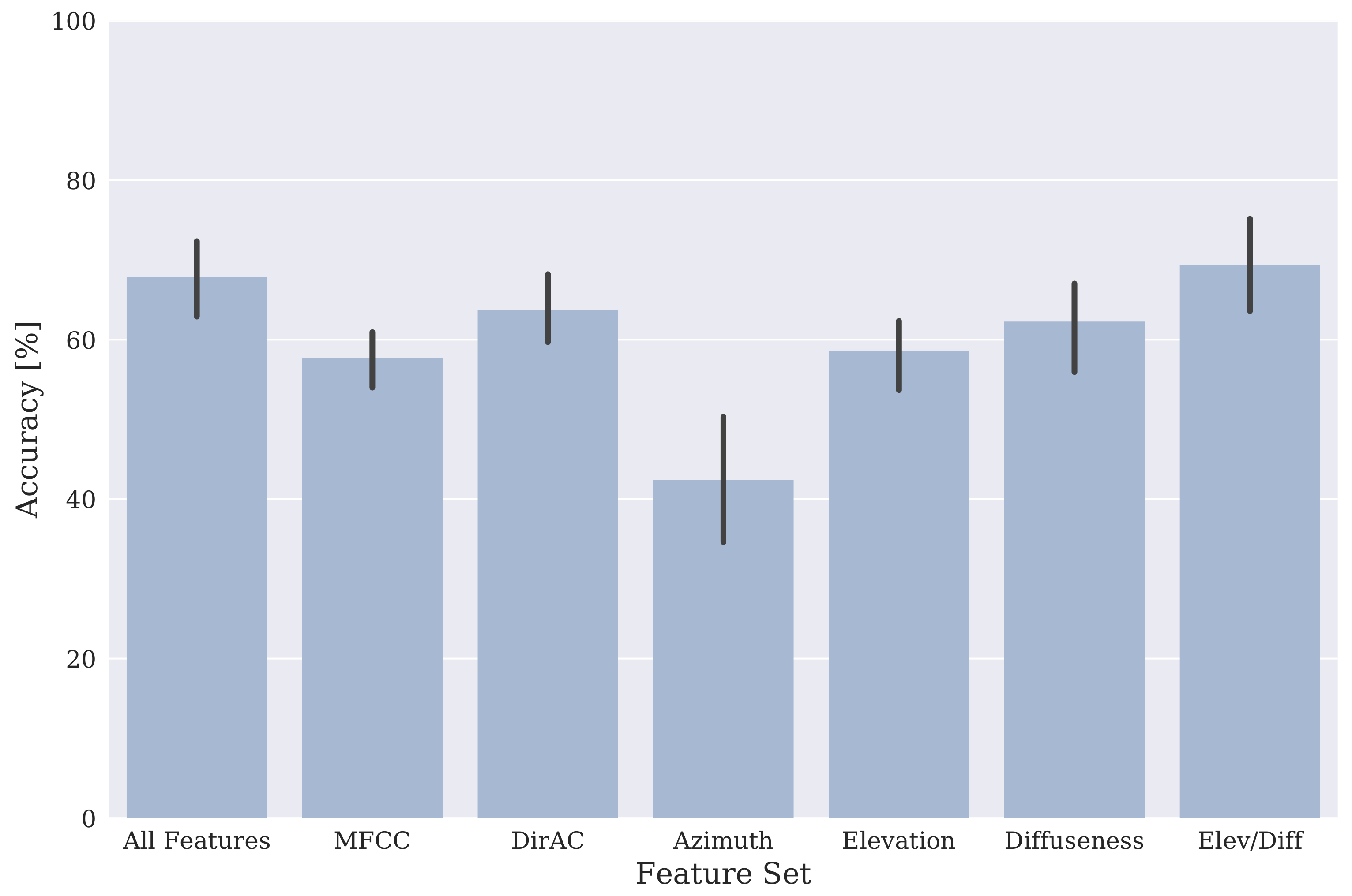
Initial analysis of this dataset previously published as part of the DCASE 2017 workshop [39] compared classification accuracies achieved using the DirAC features to those achieved when using MFCCs. In addition, classifiers were trained using individual DirAC features—azimuth, elevation and diffuseness—and a classifier was trained using a concatenation of all MFCC and DirAC features. Figure 2 shows the mean and standard deviation classification accuracies achieved across all scenes using these various feature sets. It can be seen that using all DirAC features to train a GMM classifier gives a mean accuracy of 64% across all scene classes, whereas MFCC features give a 58% mean accuracy (averaged across all folds). Azimuth data alone is much less discriminative between scenes, giving an accuracy of 43% on average, which is markedly worse than MFCCs. Elevation data, on the other hand, gives similar accuracies, and diffuseness data gives slightly better accuracies than MFCCs. The low accuracy when using azimuth data is probably attributable to the fact that azimuth estimates will be affected by the orientation of the microphone array relative to the recorded scene, whereas elevation and diffuseness should be rotation-invariant. A new classifier using elevation and diffuseness values only was therefore trained and gave an average classification accuracy of 69%, which is the best performance that was achieved. The elevation/diffuseness (E/D)—GMM classifier was therefore adopted as the baseline classifier and all further results reported here are derived from it.
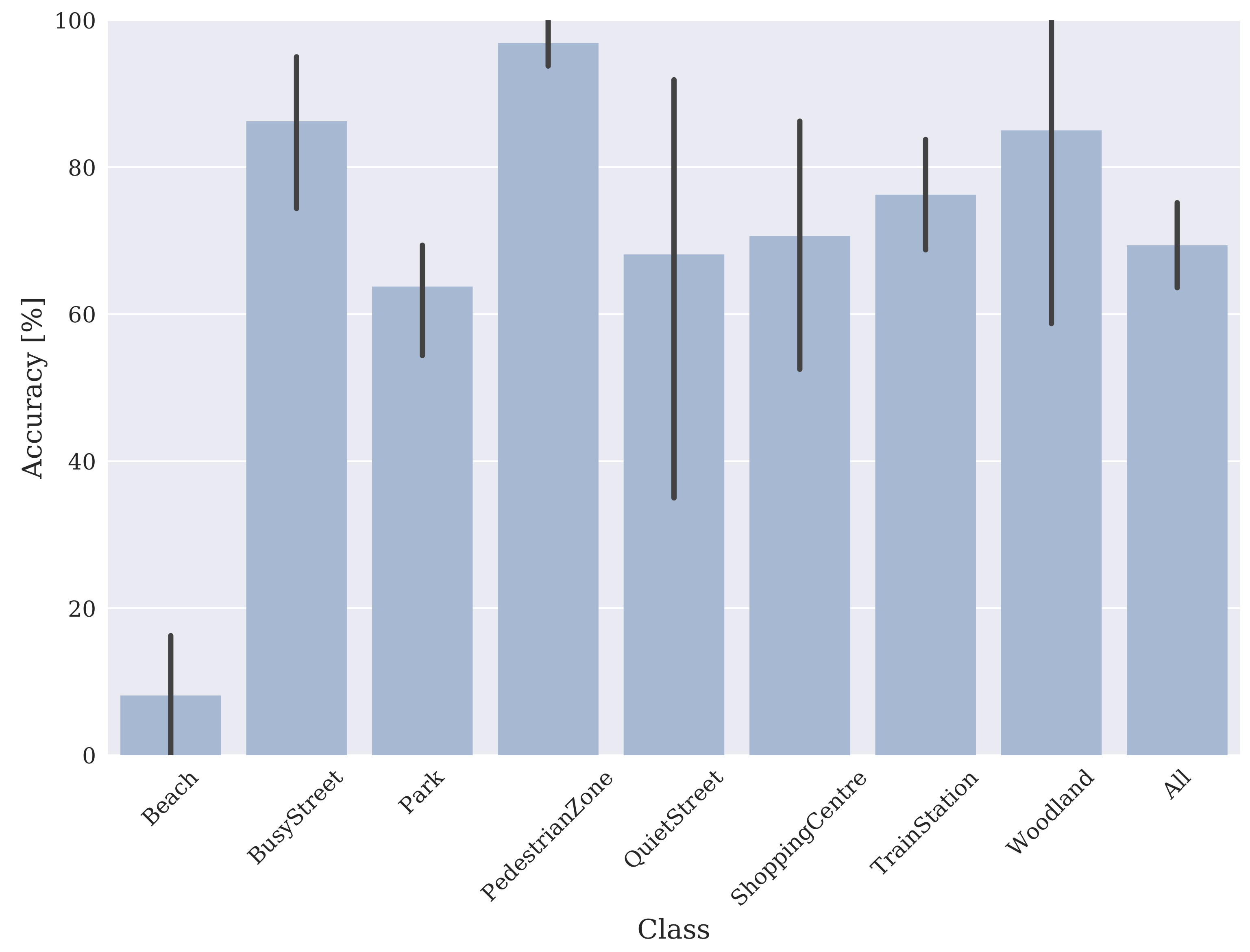
Figure 3 shows the mean and standard deviation classification accuracies from the baseline for each acoustic scene class. As previously mentioned, the mean accuracy across all scene classes is 69%. The low standard deviation (7%) indicates the dataset as a whole gives features that are fairly consistent across all folds. All of the scene classes except Beach are classified with mean accuracies above 60%. In fact, if the Beach class is discounted, the overall mean accuracy rises by 9%. Busy Street, Pedestrian Zone and Woodland are classified particularly well, at 86%, 97% and 85% accuracy, respectively. Looking at the standard deviation values for accuracy across folds could give some indication of the within-class variability between the different scene recordings. The very low standard deviation in Pedestrian Zone accuracies of 4% implies that the Pedestrian Zone recordings have very similar sonic characteristics, that is, they give very consistent features. Busy Street, Park and Train Station could be said to be moderately consistent, whereas Quiet Street, Shopping Centre and Woodland show more variability between the various recordings. The drastically lower accuracy of the Beach scene classification is very anomalous. It could be that as the primary sound source at a beach will likely be widespread and diffuse broadband noise from the ocean waves, this could yield indistinct features that could be difficult for the classifier to separate from other scenes.
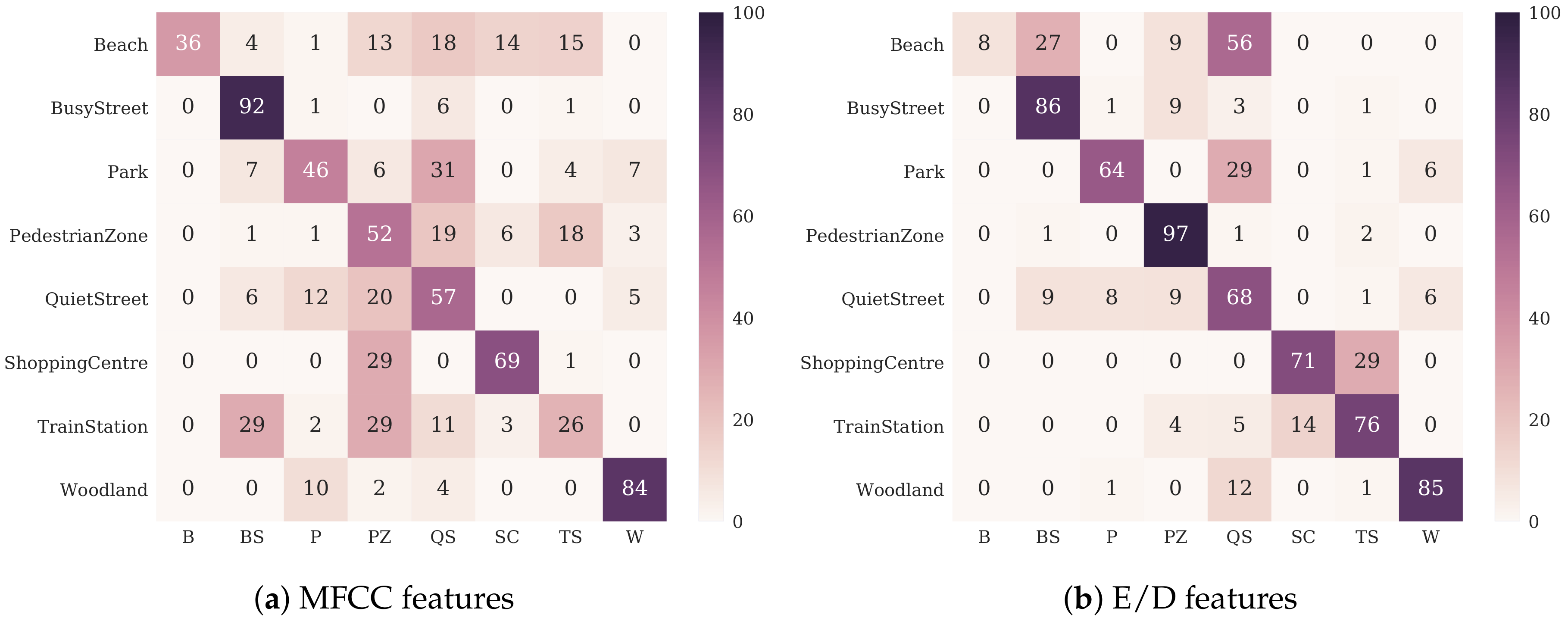
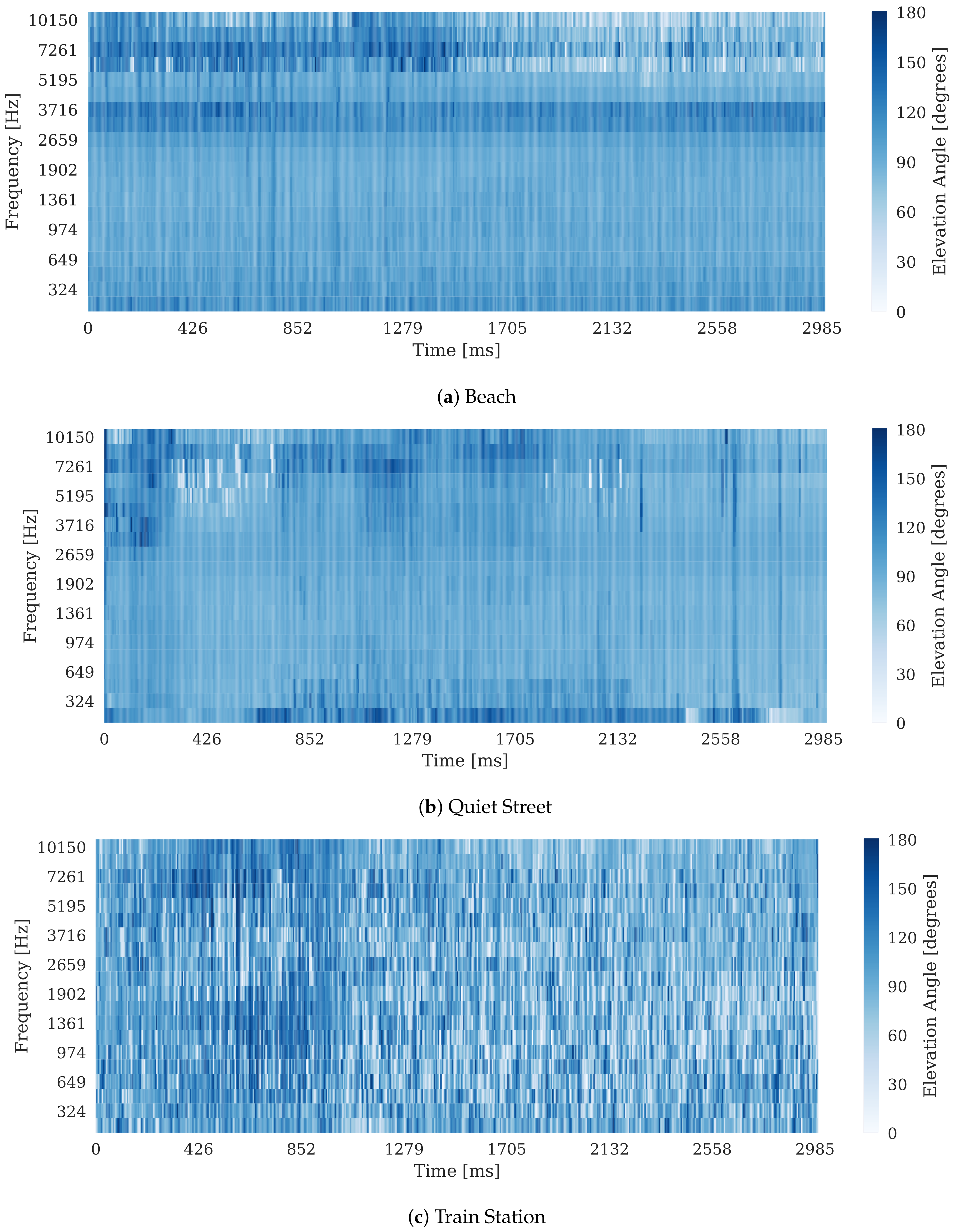
Figure 4 shows confusion matrices (previously published in [39]), which indicate classifications made by the MFCC and E/D classifiers averaged across all folds. Rows indicate the true classes and columns indicate the labels returned by the classifiers. The E/D matrix features a much more prominent leading diagonal and confusion is much less widespread than in the MFCC matrix, clearly indicating that the E/D classifier outperforms the MFCC classifier in the vast majority of cases. Beach is the only class in which the MFCC classifier significantly outperforms the E/D classifier. The most commonly-returned labels for the Beach scene by the E/D classifier are Quiet Street and Busy Street, perhaps due to the aforementioned broadband noise from ocean waves yielding spatial features similar to that of passing cars. This interpretation is corroborated by Figure 5, which shows elevation estimates extracted using Equation (3) from 30-s segments of Beach, Quiet Street and Train Station recordings as heat maps for comparison. The Beach and Quiet Street plots both show large areas across time and frequency where elevation estimates remain broadly consistent at around 90°, indicating the presence of broadband noise sources dominating around that angle. The Train Station plot, on the other hand, shows much more erratic changes in elevation estimates across time, and indeed there is no confusion between Beach and Train Station using the E/D classifier.
It is interesting to consider instances where the E/D classifier considerably outperforms the MFCC classifier, such as with Pedestrian Zone, which is classified with 97% accuracy by the E/D classifier, whereas the MFCC classifier only manages 52%. This indicates that the spatial information present in pedestrian zones is much more discriminative than the spectral information, which seems to share common features with both quiet streets and train stations. Further to this, it is interesting to investigate the instances where there is significant confusion present in both classifiers. Park, for instance, is most commonly misclassified as Quiet Street by both classifiers. This is probably due to the fact that both Park and Quiet Street scenes are both characterised as being relatively quiet locations, yet are still in the midst of urban areas. These recordings tend to contain occasional human sound and low-level background urban ‘hum’ (as opposed to Woodland, which tends to lack this). In other cases, however, the specific misclassifications do not always correspond. The most common misclassification of the Shopping Centre by the MFCC classifier is the Pedestrian Zone, a result perhaps caused by prominent human sound found in both locations. In contrast to this, for the E/D classifier the most common misclassification of the Shopping Centre is Train Station, and in fact there is no confusion with the Pedestrian Zone at all. This could be due to the similarity in acoustics between the large reverberant indoor spaces typical of train stations and shopping centres, which could have an impact on the values calculated for elevation and diffuseness.
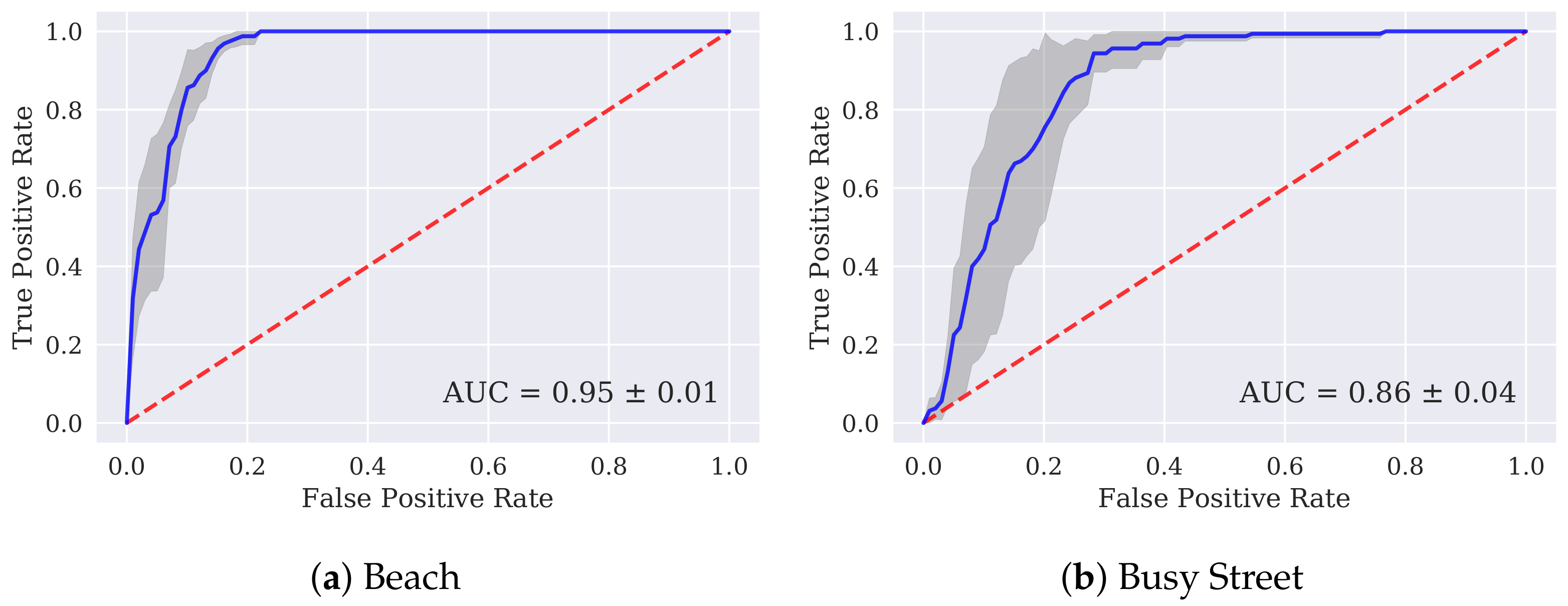
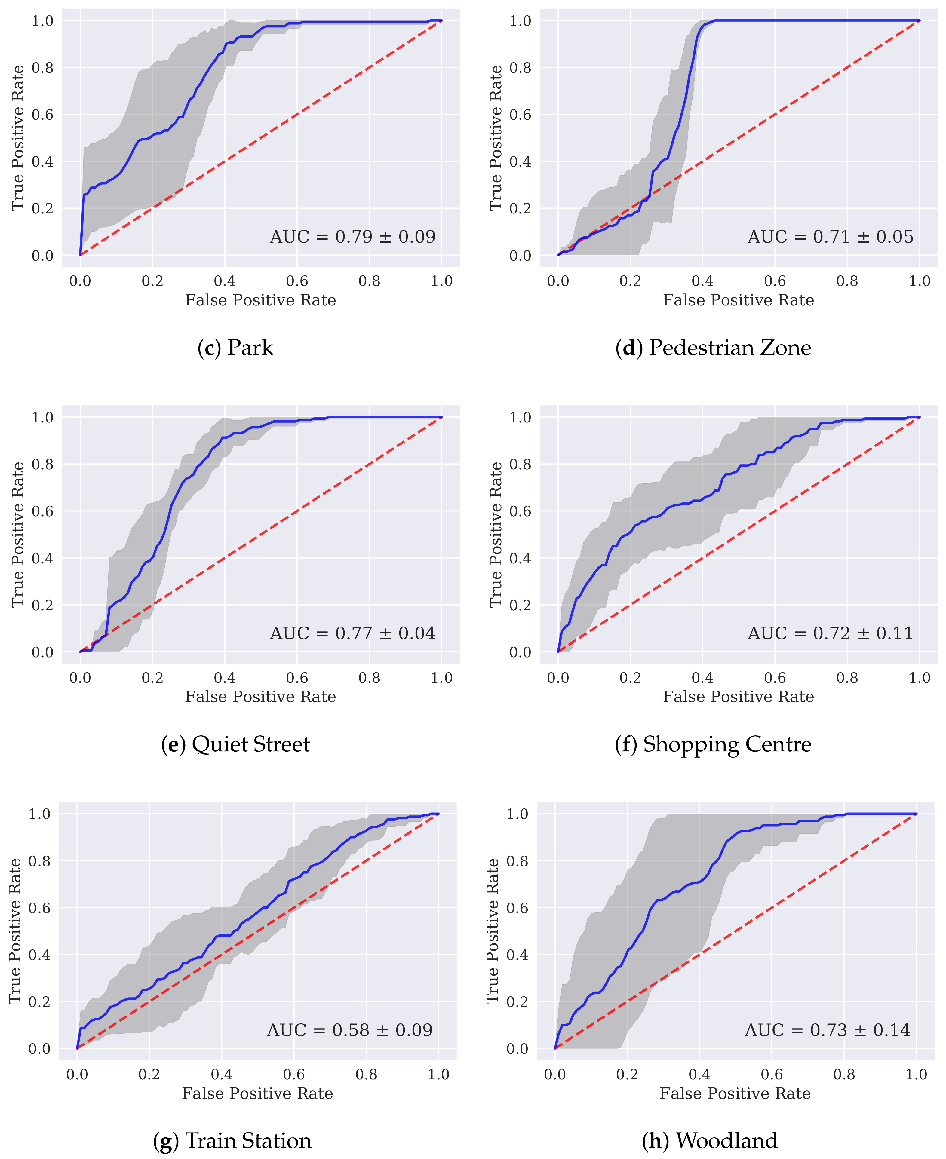
Figure 6 shows receiver operating characteristic (ROC) curves for the individual models trained to identify each location class. These curves evaluate each GMM’s performance as a one-versus-rest classifier. The curves were generated by comparing the scores generated by each model with the ground-truth labels for each scene and calculating the probabilities that a certain score will be given to a correct clip (true positive) or will be given to a clip from another scene (false positive). These pairs of probabilities are calculated for every score output from the classifier and when plotted, form the ROC curve. The larger the area under the curve (AUC), the better the classifier. The curves shown in Figure 6 show the mean ROC across the four folds. It can clearly be seen that the AUC values do not follow the pattern of the classification accuracies shown in Figure 3. This discrepancy is most stark in Figure 6a, which shows the Beach model to be the best individual classifier, with an AUC of 0.95. This indicates that the Beach model is individually very good at telling apart Beach clips from all other scenes. The very low Beach classification accuracy from the system as a whole could be explained by the fact that all the other scene models have lower AUC values than the Beach model, which suggests greater tendencies in the other models to give incorrect scenes higher probability scores.
It should be noted here that points on the ROC curves do not indicate absolute score levels. For instance, a false positive point on any given curve will not necessarily be reached at the same absolute probability score as that point on any other curve. It is therefore possible that the Beach model tends to give lower probability scores in general than the other models, and is therefore most of the the time ‘outvoted’ by other models.
These results suggest that classification accuracies could be improved by using the AUC values from each model to create confidence weightings to inform the decision making process beyond the basic summing of probability scores. A lower score from the Beach model could, for instance, carry more weight than from the Train Station model, which has an AUC of 0.58, indicating performance at only slightly higher than chance levels.
4. Discussion
The results presented in Section 3 indicate that the collation of EigenScape has been successful in that this classification exercise shows the suitability of this dataset for segmentation and cross-validation. The good, but not perfect, degree of accuracy shown by the baseline E/D-GMM classifier is very significant in that it goes some way towards showing the validity of this dataset in terms of providing a good variety of recordings. Recordings within a class label are similar enough to be grouped together by a classifier, whilst retaining an appropriate degree of variation.
These results suggest that DirAC spatial features extracted from Ambisonic audio could be viable and useful features to use for acoustic scene identification. The simplicity of the classifier used here indicates that higher accuracies could be gleaned from these features, perhaps by using a more sophisticated decision-making process, or simply more sophisticated models. Utilising temporal features could be a compelling next step in this work. It would be especially interesting to investigate whether Δ-azimuth values could be more discriminative than the azimuth values themselves, being perhaps less dependent on microphone orientation. It is also worth noting that all spatial analysis of this dataset so far has used only the first-order Ambisonic channels for feature extraction. The fourth-order channels present in this database provide much higher spatial precision that could enable more sophisticated feature extraction. The high channel count should also facilitate detailed source separation that could be used for polyphonic event detection work. Event detection within scenes should be a key area of research with this dataset moving forwards.
The size and scope of this database are such that there is a lot more knowledge to be gained than has been presented here. The findings of this paper are important initial results that indicate the investigation of spatial audio features could be a fertile new area in machine listening, especially with a view to applications in environmental sound monitoring and analysis.
Supplementary Materials
The EigenScape database is provided freely to inspire and promote research work and creativity. Please cite this paper in any published research or other work utilising this dataset. EigenScape Dataset: http://0-doi-org.brum.beds.ac.uk/10.5281/zenodo.1012809; Baseline code and segmentation tools: https://github.com/marc1701/EigenScape; Recording Map: http://bit.ly/EigenSMap.
Acknowledgments
Funding was provided by a UK Engineering and Physical Sciences Research Council (EPSRC) Doctoral Training Award, the Department of Electronic Engineering at the University of York, and in part by Digital Creativity Labs, EPSRC Grant Number: EP/M023265/1.
Author Contributions
M.G. conducted the recording work, created the baseline classifier, conducted analysis and wrote the paper. D.M. supervised the project, provided initial ideas and guidance and has acted as editor and secondary contributor to this paper.
Conflicts of Interest
The authors declare no conflict of interest.
Abbreviations
The following abbreviations are used in this manuscript:
| ASR | Automatic Speech Recognition |
| MIR | Music Information Retrieval |
| DCASE | Detection and Classification of Acoustic Scenes and Events |
| ASC | Acoustic Scene Classification |
| AED | Acoustic Event Detection |
| MFCC | Mel-Frequency Cepstral Coefficients |
| DOA | Direction of Arrival |
| DirAC | Directional Audio Coding |
| GMM | Gaussian Mixture Model |
| E/D | Elevation/Diffuseness |
| ROC | Receiver Operating Characteristic |
| AUC | Area Under the Curve |
References
- Wang, D. Computation Auditory Scene Analysis: Principles, Algorithms and Applications; Wiley: Hoboken, NJ, USA, 2006. [Google Scholar]
- Cherry, C. On Human Communication: A Review, a Survey, and a Criticism; MIT Press: Cambridge, MA, USA, 1978. [Google Scholar]
- Raś, Z. Advances in Music Information Retrieval; Springer-Verlag: Berlin/Heidelberg, Germany, 2010. [Google Scholar]
- The Magic that Makes Spotify’S Discover Weekly Playlists So Damn Good. Available online: https://qz.com/571007/the-magic-that-makes-spotifys-discover-weekly-playlists-so-damn-good/ (accessed on 18 September 2017).
- Stowell, D.; Giannoulis, D.; Benetos, E.; Lagrange, M.; Plumbley, M.D. Detection and Classification of Acoustic Scenes and Events. IEEE Trans. Multimed. 2015, 17, 1733–1746. [Google Scholar] [CrossRef]
- Barchiesi, D.; Giannoulis, D.; Stowell, D.; Plumbley, M.D. Acoustic Scene Classification: Classifying environments from the sounds they produce. IEEE Signal Process. Mag. 2015, 32, 16–34. [Google Scholar] [CrossRef] [Green Version]
- Adavanne, S.; Parascandolo, G.; Pertilä, P.; Heittola, T.; Virtanen, T. Sound Event Detection in Multisource Environments Using Spatial and Harmonic Features. In Proceedings of the Detection and Classification of Acoustic Scenes and Events, Budapest, Hungary, 3 September 2016. [Google Scholar]
- Eghbal-Zadeh, H.; Lehner, B.; Dorfer, M.; Widmer, G. CP-JKU Submissions for DCASE-2016: A Hybrid Approach Using Binaural I-Vectors and Deep Convolutional Neural Networks. In Proceedings of the Detection and Classification of Acoustic Scenes and Events, Budapest, Hungary, 3 September 2016. [Google Scholar]
- Nogueira, W.; Roma, G.; Herrera, P. Sound Scene Identification Based on MFCC, Binaural Features and a Support Vector Machine Classifier; Technical Report; IEEE AASP Challenge on Detection and Classification of Acoustic Scenes and Events; IEEE: Piscataway, NJ, USA, 2013; Available online: http://c4dm.eecs.qmul.ac.uk/sceneseventschallenge/abstracts/SC/NR1.pdf (Accessed on 6 January 2017).
- Mel Frequency Cepstral Coefficient (MFCC) Tutorial. Available online: http://practicalcryptography.com/miscellaneous/machine-learning/guide-mel-frequency-cepstral-coefficients-mfccs/ (accessed on 18 September 2017).
- Brown, A.L. Soundscapes and environmental noise management. Noise Control Eng. J. 2010, 58, 493–500. [Google Scholar] [CrossRef]
- Bunting, O.; Stammers, J.; Chesmore, D.; Bouzid, O.; Tian, G.Y.; Karatsovis, C.; Dyne, S. Instrument for Soundscape Recognition, Identification and Evaluation (ISRIE): Technology and Practical Uses. In Proceedings of the EuroNoise, Edinburgh, UK, 26–28 October 2009. [Google Scholar]
- Bunting, O.; Chesmore, D. Time frequency source separation and direction of arrival estimation in a 3D soundscape environment. Appl. Acoust. 2013, 74, 264–268. [Google Scholar] [CrossRef]
- International Standards Organisation. ISO 12913-1:2014—Acoustics—Soundscape—Part 1: Definition and Conceptual Framework; International Standards Organisation: Geneva, Switzerland, 2014. [Google Scholar]
- Davies, W.J.; Bruce, N.S.; Murphy, J.E. Soundscape Reproduction and Synthesis. Acta Acust. United Acust. 2014, 100, 285–292. [Google Scholar] [CrossRef]
- Guastavino, C.; Katz, B.F.; Polack, J.D.; Levitin, D.J.; Dubois, D. Ecological Validity of Soundscape Reproduction. Acta Acust. United Acust. 2005, 91, 333–341. [Google Scholar]
- Liu, J.; Kang, J.; Behm, H.; Luo, T. Effects of landscape on soundscape perception: Soundwalks in city parks. Landsc. Urban Plan. 2014, 123, 30–40. [Google Scholar] [CrossRef]
- Axelsson, Ö.; Nilsson, M.E.; Berglund, B. A principal components model of soundscape perception. J. Acoust. Soc. Am. 2010, 128, 2836–2846. [Google Scholar] [CrossRef] [PubMed]
- Harriet, S.; Murphy, D.T. Auralisation of an Urban Soundscape. Acta Acust. United Acust. 2015, 101, 798–810. [Google Scholar] [CrossRef]
- Lundén, P.; Axelsson, Ö.; Hurtig, M. On urban soundscape mapping: A computer can predict the outcome of soundscape assessments. In Proceedings of the Internoise, Hamburg, Germany, 21–24 August 2016; pp. 4725–4732. [Google Scholar]
- Aletta, F.; Kang, J.; Axelsson, Ö. Soundscape descriptors and a conceptual framework for developing predictive soundscape models. Landsc. Urban Plan. 2016, 149, 65–74. [Google Scholar] [CrossRef]
- Bunting, O. Sparse Seperation of Sources in 3D Soundscapes. Ph.D. Thesis, University of York, York, UK, 2010. [Google Scholar]
- Aucouturier, J.J.; Defreville, B.; Pachet, F. The Bag-of-frames Approach to Audio Pattern Recognition: A Sufficient Model for Urban Soundscapes But Not For Polyphonic Music. J. Acous. Soc. Am. 2007, 122, 881–891. [Google Scholar] [CrossRef] [PubMed]
- Lagrange, M.; Lafay, G. The bag-of-frames approach: A not so sufficient model for urban soundscapes. J. Acoust. Soc. Am. 2015, 128. [Google Scholar] [CrossRef] [PubMed]
- Mesaros, A.; Heittola, T.; Virtanen, T. TUT Database for Acoustic Scene Classification and Sound Event Detection. In Proceedings of the 24th European Signal Processing Conference (EUSIPCO), Budapest, Hungary, 28 August–2 September 2016. [Google Scholar]
- Joachim Thiemann, N.I.; Vincent, E. The Diverse Environments Multi-channel Acoustic Noise Database (DEMAND): A database of multichannel environmental noise recordings. In Proceedings of the Meetings on Acoustics, Montreal, QC, Canada, 2–7 June 2013; Volume 19. [Google Scholar]
- MH Acoustics. em32 Eigenmike® Microphone Array Release Notes; MH Acoustics: Summit, NJ, USA, 2013. [Google Scholar]
- Bates, E.; Gorzel, M.; Ferguson, L.; O’Dwyer, H.; Boland, F.M. Comparing Ambisonic Microphones—Part 1. In Proceedings of the Audio Engineering Society Conference: 2016 AES International Conference on Sound Field Control, Guildford, UK, 18–20 July 2016. [Google Scholar]
- Bates, E.; Dooney, S.; Gorzel, M.; O’Dwyer, H.; Ferguson, L.; Boland, F.M. Comparing Ambisonic Microphones—Part 2. In Proceedings of the 142nd Convention of the Audio Engineering Society, Berlin, Germany, 20–23 May 2017. [Google Scholar]
- MH Acoustics. Eigenbeam Data Specification for Eigenbeams Eigenbeam Data Specification for Eigenbeams Eigenbeam Data Specification for Eigenbeams Eigenbeam Data: Specification for Eigenbeams; MH Acoustics: Summit, NJ, USA, 2016. [Google Scholar]
- Soundfield. ST350 Portable Microphone System User Guide; Soundfield: London, UK, 2008. [Google Scholar]
- Van Grootel, M.W.W.; Andringa, T.C.; Krijnders, J.D. DARES-G1: Database of Annotated Real-world Everyday Sounds. In Proceedings of the NAG/DAGA Meeting, Rotterdam, The Netherlands, 23–26 March 2009. [Google Scholar]
- Samsung Gear 360 Camera. Available online: http://www.samsung.com/us/support/owners/product/gear-360-2016 (accessed on 8 September 2017).
- UK Data Service—Recommended Formats. Available online: https://www.ukdataservice.ac.uk/manage-data/format/recommended-formats (accessed on 11 September 2017).
- Pulkki, V. Directional audio coding in spatial sound reproduction and stereo upmixing. In Proceedings of the AES 28th International Conference, Pitea, Sweden, 30 June–2 July 2006. [Google Scholar]
- Pulkki, V. Spatial Sound Reproduction with Directional Audio Coding. J. Audio Eng. Soc. 2007, 55, 503–516. [Google Scholar]
- Pulkki, V.; Laitinen, M.V.; Vilkamo, J.; Ahonen, J.; Lokki, T.; Pihlajamäki, T. Directional audio coding—Perception-based reproduction of spatial sound. In Proceedings of the International Workshop on the Principle and Applications of Spatial Hearing, Miyagy, Japan, 11–13 November 2009. [Google Scholar]
- Kallinger, M.; Kuech, F.; Shultz-Amling, R.; Galdo, G.D.; Ahonen, J.; Pulkki, V. Analysis and adjustment of planar microphone arrays for application in Directional Audio Coding. In Proceedings of the 124th Convention of the Audio Engineering Society, Amsterdam, The Netherlands, 17–20 May 2008. [Google Scholar]
- Green, M.C.; Murphy, D. Acoustic Scene Classification Using Spatial Features. In Proceedings of the Detection and Classification of Acoustic Scenes and Events, Munich, Germany, 16–17 November 2017. [Google Scholar]
Figure 1.
The setup used to record the EigenScape database: mh-Acoustics Eigenmike within a Rycote windshield, a Samsung Gear 360 camera, an Eigenmike Microphone Interface Box, and an Apple MacBook Pro. The equipment is shown here at Redcar Beach, UK: 54°37′16′′ N, 1°04′50′′W.
Figure 1.
The setup used to record the EigenScape database: mh-Acoustics Eigenmike within a Rycote windshield, a Samsung Gear 360 camera, an Eigenmike Microphone Interface Box, and an Apple MacBook Pro. The equipment is shown here at Redcar Beach, UK: 54°37′16′′ N, 1°04′50′′W.

Figure 2.
Mean and standard deviation classification accuracies across all folds for the entire dataset using various different feature sets (from [39]). MFCC: Mel-frequency cepstral coefficient; DirAC: directional audio coding.
Figure 2.
Mean and standard deviation classification accuracies across all folds for the entire dataset using various different feature sets (from [39]). MFCC: Mel-frequency cepstral coefficient; DirAC: directional audio coding.

Figure 3.
Mean and standard deviation classification accuracies across all folds for each scene class using the elevation/diffuseness–Gaussian mixture model (E/D-GMM) classifier.
Figure 3.
Mean and standard deviation classification accuracies across all folds for each scene class using the elevation/diffuseness–Gaussian mixture model (E/D-GMM) classifier.

Figure 4.
Confusion matrices of classifiers trained using MFCC features and elevation/diffuseness features extracted using DirAC. Figures indicate classification percentages across all folds (from [39]).
Figure 4.
Confusion matrices of classifiers trained using MFCC features and elevation/diffuseness features extracted using DirAC. Figures indicate classification percentages across all folds (from [39]).

Figure 5.
Heat maps depicting elevation estimates extracted from 30-s segments of Beach, Quiet Street and Train Station recordings.
Figure 5.
Heat maps depicting elevation estimates extracted from 30-s segments of Beach, Quiet Street and Train Station recordings.

Figure 6.
Receiver operating characteristics (ROC) curves for each scene classifier, showing mean (solid line) and standard deviation (grey area) of the curves calculated using results across all folds. Dotted line represents chance performance. AUC: area under the curve.
Figure 6.
Receiver operating characteristics (ROC) curves for each scene classifier, showing mean (solid line) and standard deviation (grey area) of the curves calculated using results across all folds. Dotted line represents chance performance. AUC: area under the curve.


© 2017 by the authors. Licensee MDPI, Basel, Switzerland. This article is an open access article distributed under the terms and conditions of the Creative Commons Attribution (CC BY) license (http://creativecommons.org/licenses/by/4.0/).
Share and Cite
MDPI and ACS Style
Green, M.C.; Murphy, D. EigenScape: A Database of Spatial Acoustic Scene Recordings. Appl. Sci. 2017, 7, 1204. https://0-doi-org.brum.beds.ac.uk/10.3390/app7111204
AMA Style
Green MC, Murphy D. EigenScape: A Database of Spatial Acoustic Scene Recordings. Applied Sciences. 2017; 7(11):1204. https://0-doi-org.brum.beds.ac.uk/10.3390/app7111204
Chicago/Turabian StyleGreen, Marc Ciufo, and Damian Murphy. 2017. "EigenScape: A Database of Spatial Acoustic Scene Recordings" Applied Sciences 7, no. 11: 1204. https://0-doi-org.brum.beds.ac.uk/10.3390/app7111204
Note that from the first issue of 2016, this journal uses article numbers instead of page numbers. See further details here.