An NHPP Software Reliability Model with S-Shaped Growth Curve Subject to Random Operating Environments and Optimal Release Time

Abstract
:1. Introduction
2. A New NHPP Software Reliability Model
2.1. Non-Homogeneous Poisson Process
- (I)
- (II)
- Independent increments
- (III)
- , (): the average of the number of failures in the interval []
2.2. General NHPP Software Reliability Model
2.3. New NHPP Software Reliability Model
| (a) | The occurrence of a software failure follows a non-homogeneous Poisson process. |
| (b) | Faults during execution can cause software failure. |
| (c) | The software failure detection rate at any time depends on both the fault detection rate and the number of remaining faults in the software at that time. |
| (d) | Debugging is performed to remove faults immediately when a software failure occurs. |
| (e) | New faults may be introduced into the software system, regardless of whether other faults are removed or not. |
| (f) | The fault detection rate can be expressed by (6). |
| (g) | The random operating environment is captured if unit failure detection rate is multiplied by a factor that represents the uncertainty of the system fault detection rate in the field |
3. Criteria for Model Comparisons
4. Optimal Software Release Policy
5. Numerical Examples
5.1. Data Information
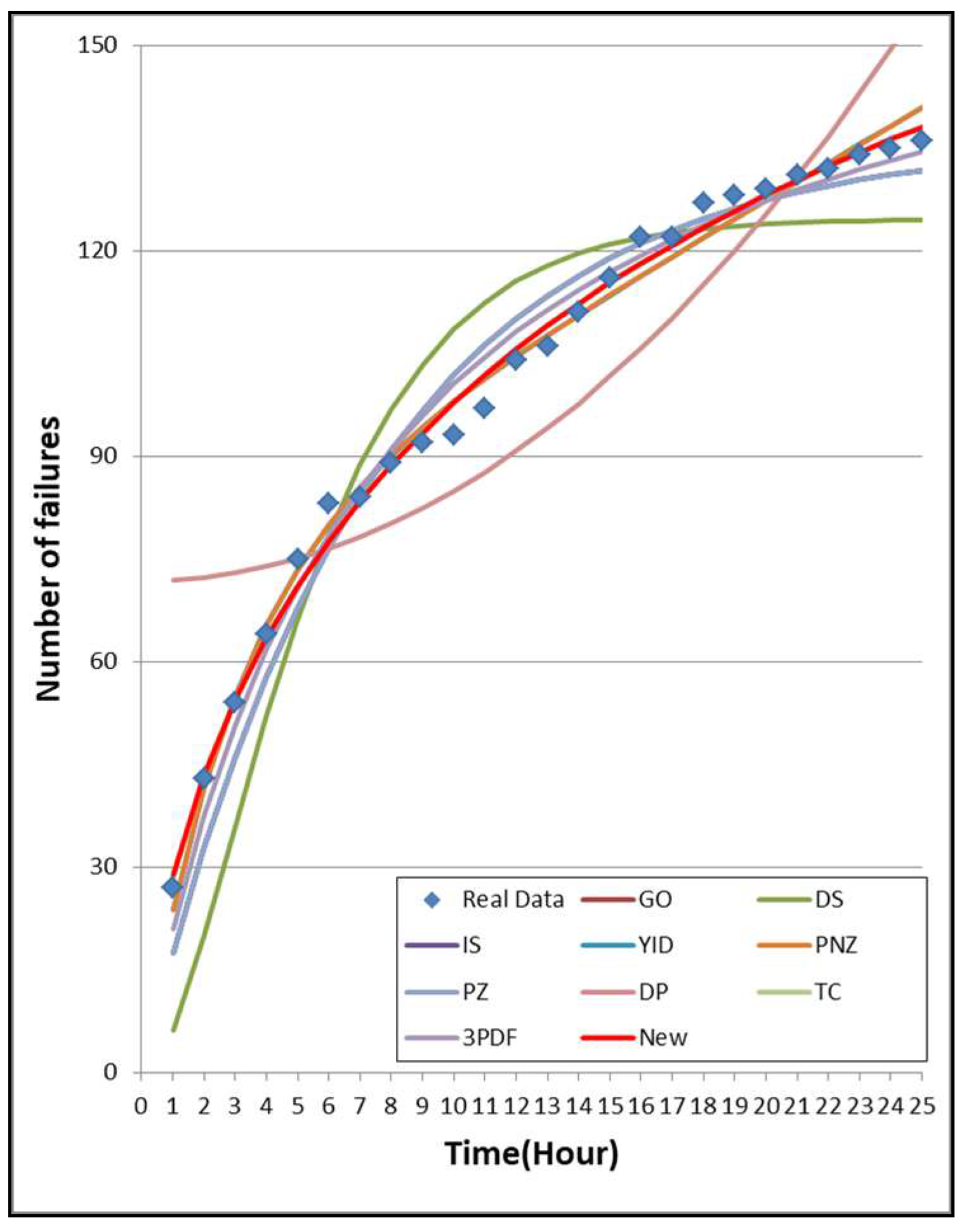
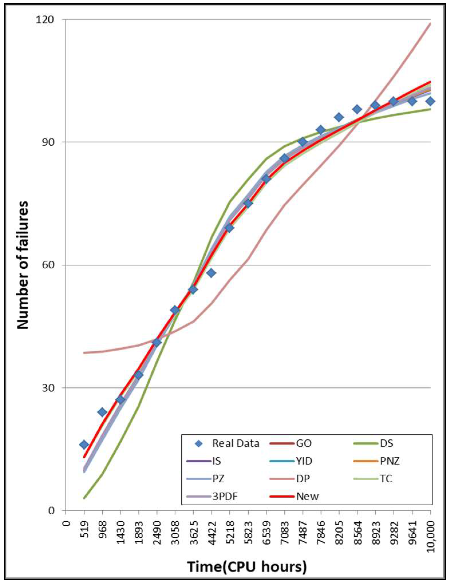
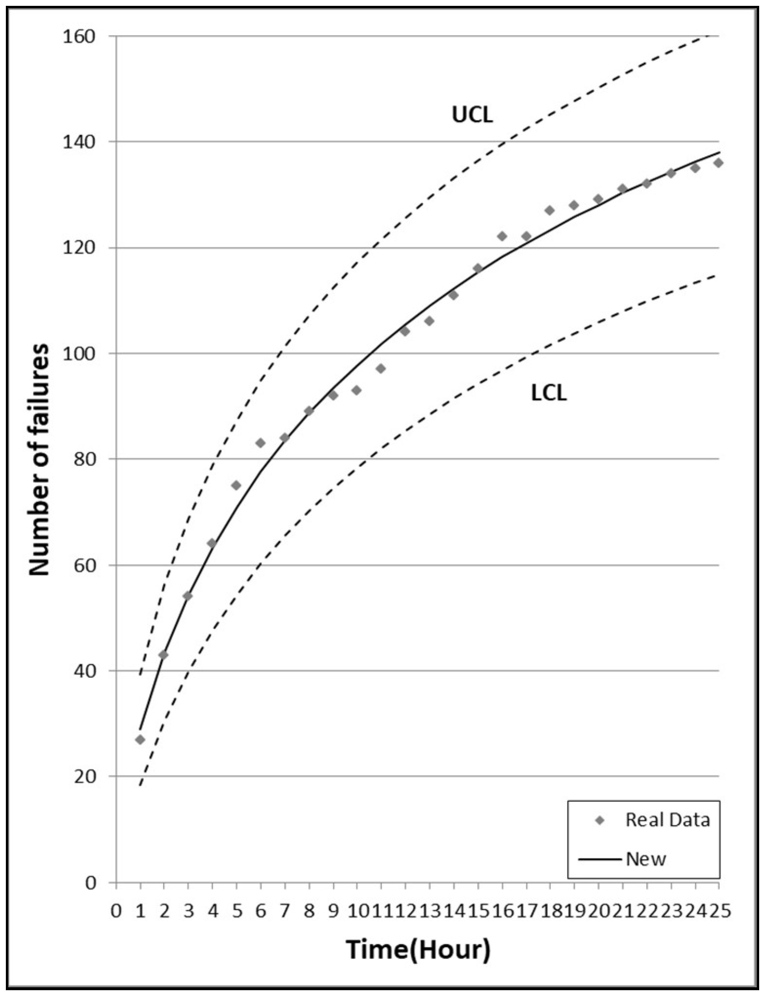
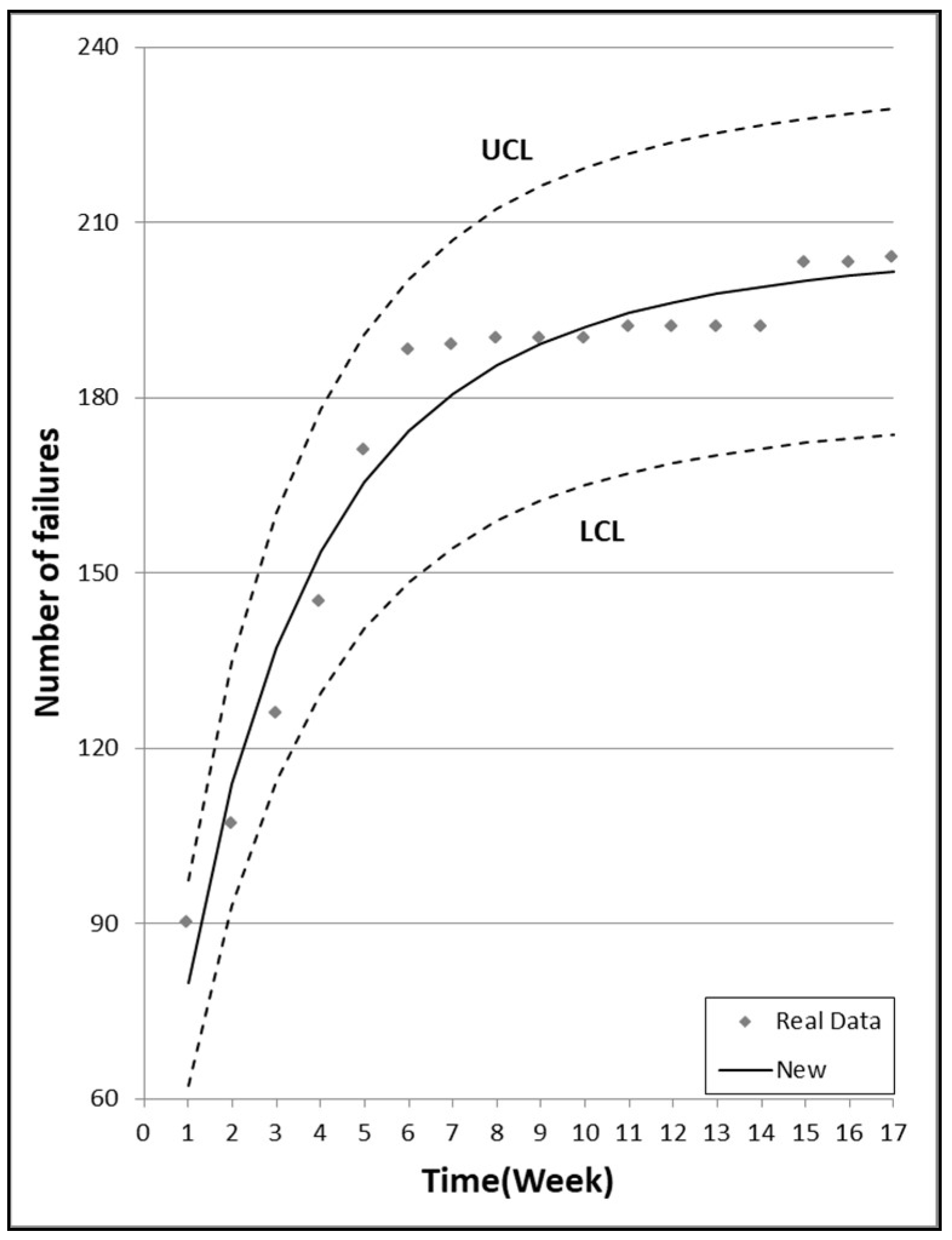
5.2. Model Analysis
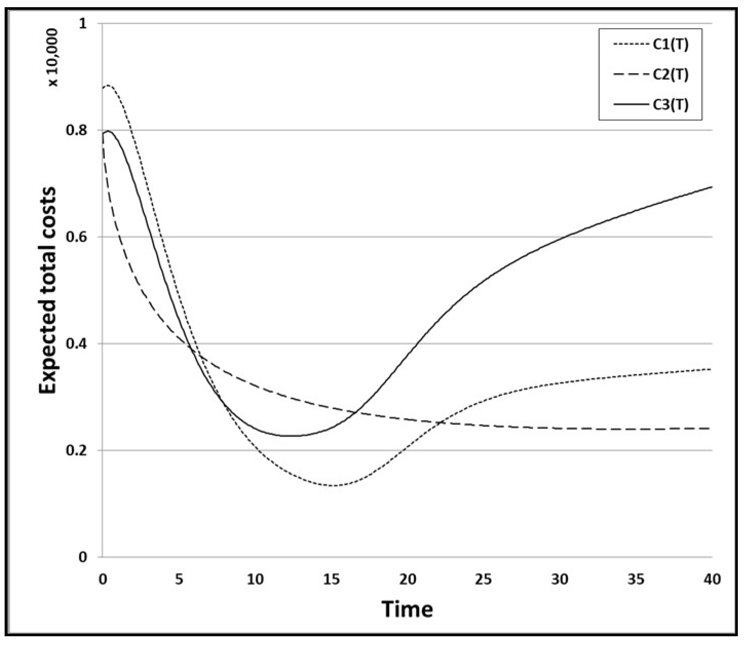
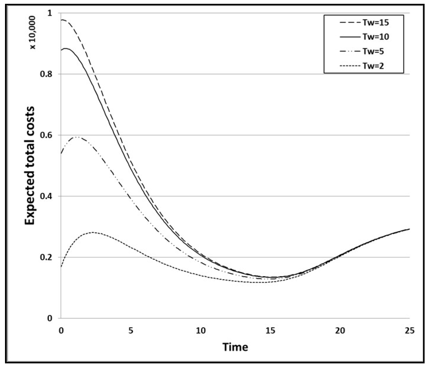
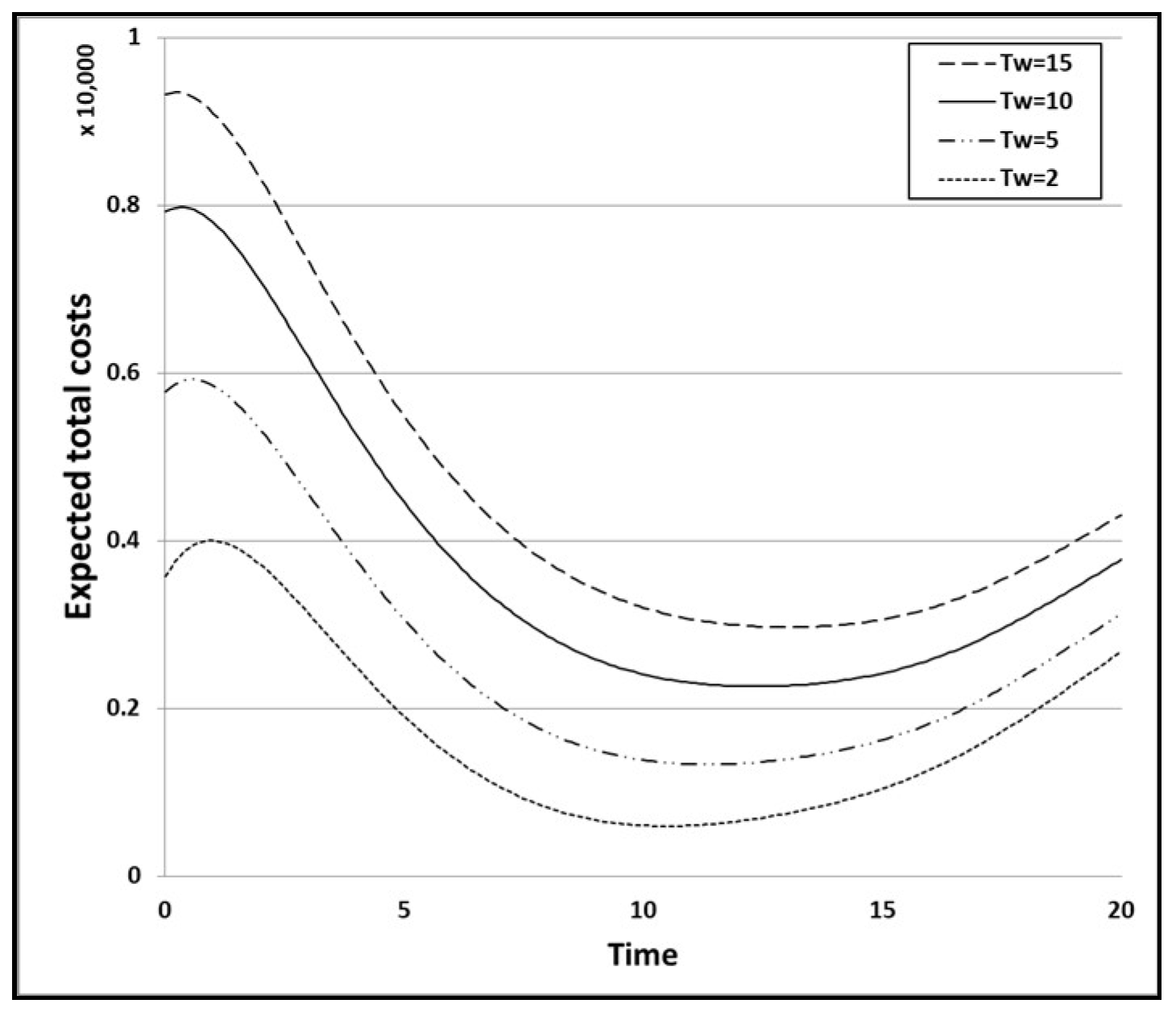
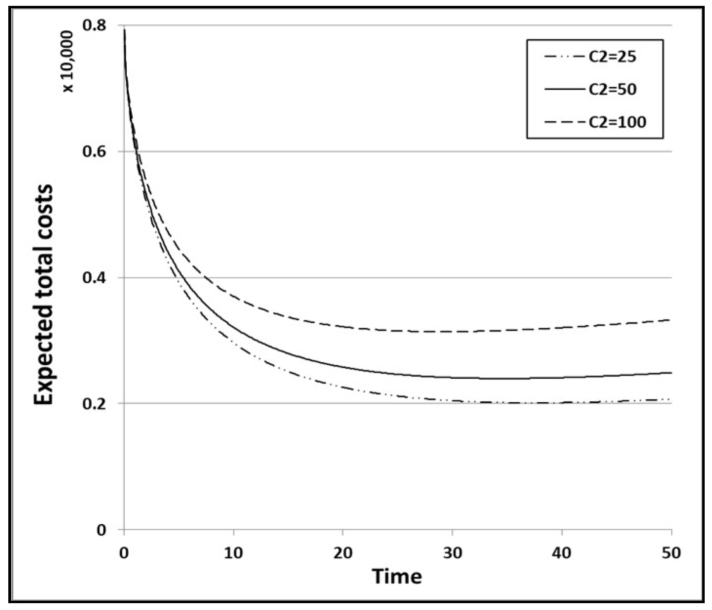
5.3. Optimal Software Release Time
6. Conclusions
Acknowledgements
Author Contributions
Conflicts of Interest
Appendix A

| Model | Time Index | 1 | 2 | 3 | 4 | 5 | 6 | 7 | 8 | 9 | |||||
| GOM | LCL | 9.329 | 21.586 | 32.810 | 42.823 | 51.671 | 59.452 | 66.277 | 72.253 | 77.479 | |||||
| 17.537 | 32.814 | 46.121 | 57.713 | 67.811 | 76.607 | 84.269 | 90.944 | 96.758 | |||||||
| UCL | 25.745 | 44.041 | 59.431 | 72.602 | 83.950 | 93.761 | 102.261 | 109.635 | 116.037 | ||||||
| DSM | LCL | 1.352 | 11.192 | 24.289 | 37.792 | 50.271 | 61.120 | 70.191 | 77.571 | 83.458 | |||||
| 6.253 | 19.945 | 36.058 | 51.914 | 66.220 | 78.484 | 88.644 | 96.861 | 103.387 | |||||||
| UCL | 11.154 | 28.698 | 47.827 | 66.035 | 82.170 | 95.847 | 107.097 | 116.150 | 123.316 | ||||||
| ISM | LCL | 9.328 | 21.584 | 32.808 | 42.820 | 51.668 | 59.449 | 66.274 | 72.250 | 77.476 | |||||
| 17.535 | 32.811 | 46.118 | 57.709 | 67.807 | 76.603 | 84.266 | 90.941 | 96.755 | |||||||
| UCL | 25.743 | 44.038 | 59.428 | 72.599 | 83.947 | 93.758 | 102.258 | 109.631 | 116.034 | ||||||
| YIDM | LCL | 14.263 | 28.936 | 40.449 | 49.466 | 56.637 | 62.468 | 67.333 | 71.506 | 75.185 | |||||
| 23.831 | 41.573 | 54.982 | 65.305 | 73.433 | 79.998 | 85.451 | 90.111 | 94.209 | |||||||
| UCL | 33.399 | 54.211 | 69.515 | 81.144 | 90.228 | 97.528 | 103.568 | 108.717 | 113.232 | ||||||
| PNZM | LCL | 14.191 | 28.840 | 40.360 | 49.400 | 56.598 | 62.455 | 67.343 | 71.534 | 75.227 | |||||
| 23.741 | 41.460 | 54.879 | 65.230 | 73.389 | 79.984 | 85.462 | 90.143 | 94.255 | |||||||
| UCL | 33.291 | 54.080 | 69.399 | 81.059 | 90.179 | 97.513 | 103.581 | 108.752 | 113.283 | ||||||
| PZM | LCL | 9.329 | 21.586 | 32.810 | 42.823 | 51.671 | 59.452 | 66.277 | 72.253 | 77.479 | |||||
| 17.537 | 32.813 | 46.121 | 57.713 | 67.811 | 76.607 | 84.269 | 90.944 | 96.758 | |||||||
| UCL | 25.745 | 44.041 | 59.431 | 72.602 | 83.950 | 93.761 | 102.261 | 109.635 | 116.037 | ||||||
| DPM | LCL | 55.306 | 55.649 | 56.223 | 57.028 | 58.068 | 59.344 | 60.859 | 62.614 | 64.611 | |||||
| 71.929 | 72.316 | 72.964 | 73.874 | 75.047 | 76.485 | 78.189 | 80.162 | 82.403 | |||||||
| UCL | 88.551 | 88.984 | 89.706 | 90.720 | 92.026 | 93.626 | 95.520 | 97.710 | 100.195 | ||||||
| TCM | LCL | 17.974 | 30.408 | 39.981 | 47.851 | 54.561 | 60.419 | 65.621 | 70.302 | 74.555 | |||||
| 28.423 | 43.306 | 54.443 | 63.465 | 71.086 | 77.695 | 83.535 | 88.768 | 93.508 | |||||||
| UCL | 38.872 | 56.204 | 68.905 | 79.080 | 87.611 | 94.971 | 101.449 | 107.234 | 112.461 | ||||||
| 3PFDM | LCL | 12.011 | 25.458 | 36.751 | 46.227 | 54.252 | 61.123 | 67.065 | 72.251 | 76.816 | |||||
| 20.991 | 37.452 | 50.708 | 61.611 | 70.737 | 78.487 | 85.151 | 90.942 | 96.021 | |||||||
| UCL | 29.970 | 49.447 | 64.665 | 76.995 | 87.221 | 95.851 | 103.237 | 109.633 | 115.227 | ||||||
| New | LCL | 18.358 | 30.526 | 39.950 | 47.745 | 54.426 | 60.283 | 65.501 | 70.208 | 74.492 | |||||
| 28.893 | 43.444 | 54.407 | 63.344 | 70.933 | 77.542 | 83.401 | 88.663 | 93.438 | |||||||
| UCL | 39.428 | 56.363 | 68.864 | 78.944 | 87.440 | 94.801 | 101.300 | 107.118 | 112.384 | ||||||
| Model | Time Index | 10 | 11 | 12 | 13 | 14 | 15 | 16 | 17 | ||||||
| GOM | LCL | 82.045 | 86.033 | 89.514 | 92.552 | 95.201 | 97.512 | 99.527 | 101.284 | ||||||
| 101.823 | 106.235 | 110.078 | 113.426 | 116.342 | 118.882 | 121.095 | 123.023 | ||||||||
| UCL | 121.600 | 126.436 | 130.641 | 134.300 | 137.483 | 140.253 | 142.663 | 144.762 | |||||||
| DSM | LCL | 88.083 | 91.672 | 94.431 | 96.534 | 98.127 | 99.326 | 100.225 | 100.895 | ||||||
| 108.498 | 112.457 | 115.494 | 117.807 | 119.557 | 120.874 | 121.861 | 122.596 | ||||||||
| UCL | 128.914 | 133.241 | 136.557 | 139.080 | 140.988 | 142.423 | 143.497 | 144.298 | |||||||
| ISM | LCL | 82.043 | 86.031 | 89.512 | 92.550 | 95.200 | 97.511 | 99.526 | 101.283 | ||||||
| 101.820 | 106.232 | 110.076 | 113.424 | 116.340 | 118.881 | 121.094 | 123.022 | ||||||||
| UCL | 121.597 | 126.434 | 130.639 | 134.298 | 137.481 | 140.251 | 142.662 | 144.761 | |||||||
| YIDM | LCL | 78.512 | 81.588 | 84.485 | 87.257 | 89.939 | 92.558 | 95.133 | 97.678 | ||||||
| 97.905 | 101.316 | 104.523 | 107.586 | 110.546 | 113.433 | 116.267 | 119.064 | ||||||||
| UCL | 117.298 | 121.044 | 124.561 | 127.916 | 131.153 | 134.307 | 137.401 | 140.451 | |||||||
| PNZM | LCL | 78.562 | 81.642 | 84.540 | 87.310 | 89.987 | 92.600 | 95.168 | 97.703 | ||||||
| 97.960 | 101.376 | 104.584 | 107.645 | 110.600 | 113.479 | 116.305 | 119.092 | ||||||||
| UCL | 117.359 | 121.110 | 124.628 | 127.980 | 131.212 | 134.358 | 137.442 | 140.481 | |||||||
| PZM | LCL | 82.045 | 86.033 | 89.514 | 92.552 | 95.201 | 97.512 | 99.527 | 101.284 | ||||||
| 101.823 | 106.235 | 110.078 | 113.426 | 116.342 | 118.882 | 121.095 | 123.023 | ||||||||
| UCL | 121.600 | 126.436 | 130.641 | 134.300 | 137.483 | 140.253 | 142.663 | 144.762 | |||||||
| DPM | LCL | 66.855 | 69.346 | 72.087 | 75.081 | 78.331 | 81.838 | 85.606 | 89.636 | ||||||
| 84.916 | 87.701 | 90.759 | 94.093 | 97.704 | 101.593 | 105.762 | 110.212 | ||||||||
| UCL | 102.977 | 106.055 | 109.432 | 113.105 | 117.078 | 121.348 | 125.918 | 130.788 | |||||||
| TCM | LCL | 78.453 | 82.050 | 85.387 | 88.500 | 91.416 | 94.157 | 96.744 | 99.191 | ||||||
| 97.840 | 101.828 | 105.521 | 108.959 | 112.174 | 115.193 | 118.038 | 120.726 | ||||||||
| UCL | 117.227 | 121.606 | 125.654 | 129.418 | 132.933 | 136.229 | 139.332 | 142.261 | |||||||
| 3PFDM | LCL | 80.863 | 84.475 | 87.718 | 90.647 | 93.303 | 95.724 | 97.940 | 99.974 | ||||||
| 100.512 | 104.512 | 108.096 | 111.326 | 114.253 | 116.917 | 119.352 | 121.586 | ||||||||
| UCL | 120.162 | 124.549 | 128.473 | 132.006 | 135.203 | 138.110 | 140.764 | 143.198 | |||||||
| New | LCL | 78.423 | 82.051 | 85.417 | 88.555 | 91.491 | 94.248 | 96.844 | 99.296 | ||||||
| 97.806 | 101.829 | 105.554 | 109.019 | 112.257 | 115.293 | 118.148 | 120.841 | ||||||||
| UCL | 117.189 | 121.607 | 125.690 | 129.484 | 133.024 | 136.338 | 139.452 | 142.387 | |||||||
| Model | Time Index | 18 | 19 | 20 | 21 | 22 | 23 | 24 | 25 | ||||||
| GOM | LCL | 102.8153 | 104.15 | 105.3133 | 106.3271 | 107.2106 | 107.9804 | 108.6512 | 109.2357 | ||||||
| 124.7022 | 126.165 | 127.4392 | 128.5491 | 129.516 | 130.3582 | 131.0919 | 131.731 | ||||||||
| UCL | 146.5892 | 148.1799 | 149.565 | 150.7711 | 151.8214 | 152.736 | 153.5326 | 154.2263 | |||||||
| DSM | LCL | 101.3931 | 101.7621 | 102.0346 | 102.2353 | 102.3828 | 102.4909 | 102.57 | 102.6278 | ||||||
| 123.1427 | 123.5475 | 123.8463 | 124.0664 | 124.2281 | 124.3466 | 124.4333 | 124.4967 | ||||||||
| UCL | 144.8924 | 145.3328 | 145.658 | 145.8975 | 146.0734 | 146.2023 | 146.2967 | 146.3656 | |||||||
| ISM | LCL | 102.8143 | 104.1492 | 105.3126 | 106.3265 | 107.21 | 107.9799 | 108.6508 | 109.2353 | ||||||
| 124.7012 | 126.164 | 127.4383 | 128.5484 | 129.5154 | 130.3577 | 131.0914 | 131.7306 | ||||||||
| UCL | 146.588 | 148.1789 | 149.5641 | 150.7703 | 151.8207 | 152.7354 | 153.5321 | 154.2259 | |||||||
| YIDM | LCL | 100.2015 | 102.7107 | 105.2103 | 107.7037 | 110.1934 | 112.6811 | 115.1679 | 117.6547 | ||||||
| 121.8354 | 124.5875 | 127.3263 | 130.0555 | 132.7779 | 135.4956 | 138.2097 | 140.9215 | ||||||||
| UCL | 143.4693 | 146.4644 | 149.4423 | 152.4073 | 155.3625 | 158.31 | 161.2516 | 164.1883 | |||||||
| PNZM | LCL | 100.2169 | 102.7154 | 105.2037 | 107.6855 | 110.1632 | 112.6385 | 115.1129 | 117.587 | ||||||
| 121.8523 | 124.5927 | 127.3191 | 130.0356 | 132.7449 | 135.4491 | 138.1497 | 140.8477 | ||||||||
| UCL | 143.4877 | 146.47 | 149.4345 | 152.3856 | 155.3266 | 158.2597 | 161.1866 | 164.1084 | |||||||
| PZM | LCL | 102.8153 | 104.15 | 105.3133 | 106.3271 | 107.2106 | 107.9804 | 108.6512 | 109.2357 | ||||||
| 124.7022 | 126.165 | 127.4392 | 128.5491 | 129.516 | 130.3582 | 131.0919 | 131.731 | ||||||||
| UCL | 146.5892 | 148.1799 | 149.565 | 150.7711 | 151.8214 | 152.736 | 153.5326 | 154.2263 | |||||||
| DPM | LCL | 93.93128 | 98.49414 | 103.3268 | 108.4316 | 113.8108 | 119.4664 | 125.4007 | 131.6157 | ||||||
| 114.9445 | 119.961 | 125.2629 | 130.8518 | 136.7288 | 142.8956 | 149.3535 | 156.1038 | ||||||||
| UCL | 135.9577 | 141.4278 | 147.199 | 153.2719 | 159.6469 | 166.3248 | 173.3063 | 180.5919 | |||||||
| TCM | LCL | 101.5124 | 103.7205 | 105.8252 | 107.8352 | 109.7585 | 111.6019 | 113.3714 | 115.0726 | ||||||
| 123.2736 | 125.6944 | 127.9996 | 130.1994 | 132.3026 | 134.3169 | 136.2493 | 138.1057 | ||||||||
| UCL | 145.0349 | 147.6682 | 150.174 | 152.5635 | 154.8467 | 157.032 | 159.1271 | 161.1389 | |||||||
| 3PFDM | LCL | 101.8497 | 103.5836 | 105.1914 | 106.6864 | 108.0801 | 109.3824 | 110.6019 | 111.7464 | ||||||
| 123.6436 | 125.5443 | 127.3057 | 128.9424 | 130.4673 | 131.8914 | 133.2244 | 134.4748 | ||||||||
| UCL | 145.4374 | 147.505 | 149.4199 | 151.1983 | 152.8544 | 154.4004 | 155.8469 | 157.2032 | |||||||
| New | LCL | 101.6161 | 103.8169 | 105.9085 | 107.8999 | 109.799 | 111.6129 | 113.3476 | 115.009 | ||||||
| 123.3873 | 125.8 | 128.0908 | 130.2702 | 132.3469 | 134.3289 | 136.2233 | 138.0364 | ||||||||
| UCL | 145.1586 | 147.783 | 150.2732 | 152.6404 | 154.8947 | 157.045 | 159.099 | 161.0638 | |||||||
| Model | Time Index | 1 | 2 | 3 | 4 | 5 | 6 | 7 | 8 | 9 | |||||||
| GOM | LCL | 49.147 | 88.100 | 114.753 | 132.788 | 144.944 | 153.123 | 158.620 | 162.312 | 164.791 | |||||||
| 64.942 | 108.518 | 137.757 | 157.376 | 170.540 | 179.373 | 185.300 | 189.276 | 191.945 | |||||||||
| UCL | 80.737 | 128.935 | 160.761 | 181.963 | 196.135 | 205.623 | 211.980 | 216.241 | 219.099 | ||||||||
| DSM | LCL | 29.754 | 81.610 | 119.319 | 141.607 | 153.581 | 159.671 | 162.660 | 164.090 | 164.762 | |||||||
| 42.537 | 101.340 | 142.735 | 166.930 | 179.867 | 186.433 | 189.651 | 191.191 | 191.914 | |||||||||
| UCL | 55.320 | 121.071 | 166.151 | 192.253 | 206.153 | 213.194 | 216.643 | 218.291 | 219.066 | ||||||||
| ISM | LCL | 49.138 | 88.084 | 114.731 | 132.764 | 144.918 | 153.095 | 158.591 | 162.282 | 164.761 | |||||||
| 64.931 | 108.500 | 137.733 | 157.349 | 170.511 | 179.343 | 185.269 | 189.245 | 191.913 | |||||||||
| UCL | 80.725 | 128.915 | 160.736 | 181.935 | 196.104 | 205.590 | 211.946 | 216.207 | 219.065 | ||||||||
| YIDM | LCL | 51.989 | 90.820 | 116.125 | 132.604 | 143.452 | 150.736 | 155.770 | 159.386 | 162.108 | |||||||
| 68.171 | 111.517 | 139.254 | 157.176 | 168.926 | 176.797 | 182.228 | 186.125 | 189.057 | |||||||||
| UCL | 84.354 | 132.215 | 162.383 | 181.748 | 194.400 | 202.858 | 208.686 | 212.864 | 216.007 | ||||||||
| PNZM | LCL | 51.946 | 90.780 | 116.107 | 132.609 | 143.476 | 150.772 | 155.811 | 159.427 | 162.145 | |||||||
| 68.123 | 111.474 | 139.234 | 157.181 | 168.952 | 176.835 | 182.272 | 186.169 | 189.097 | |||||||||
| UCL | 84.300 | 132.168 | 162.361 | 181.753 | 194.428 | 202.899 | 208.733 | 212.912 | 216.049 | ||||||||
| PZM | LCL | 49.064 | 88.017 | 114.677 | 132.724 | 144.892 | 153.080 | 158.585 | 162.284 | 164.769 | |||||||
| 64.848 | 108.425 | 137.674 | 157.306 | 170.483 | 179.327 | 185.263 | 189.247 | 191.921 | |||||||||
| UCL | 80.631 | 128.834 | 160.672 | 181.888 | 196.074 | 205.573 | 211.940 | 216.210 | 219.074 | ||||||||
| DPM | LCL | 123.469 | 124.167 | 125.336 | 126.981 | 129.105 | 131.715 | 134.816 | 138.411 | 142.507 | |||||||
| 147.252 | 148.012 | 149.283 | 151.071 | 153.379 | 156.212 | 159.574 | 163.470 | 167.904 | |||||||||
| UCL | 171.036 | 171.857 | 173.230 | 175.161 | 177.652 | 180.709 | 184.333 | 188.529 | 193.301 | ||||||||
| TCM | LCL | 60.749 | 93.551 | 114.901 | 129.743 | 140.446 | 148.355 | 154.305 | 158.844 | 162.346 | |||||||
| 78.066 | 114.526 | 137.919 | 154.071 | 165.673 | 174.225 | 180.648 | 185.542 | 189.313 | |||||||||
| UCL | 95.384 | 135.501 | 160.936 | 178.399 | 190.901 | 200.096 | 206.991 | 212.239 | 216.281 | ||||||||
| 3PFDM | LCL | 57.549 | 93.474 | 115.850 | 130.807 | 141.307 | 148.941 | 154.636 | 158.970 | 162.319 | |||||||
| 74.461 | 114.441 | 138.954 | 155.226 | 166.605 | 174.858 | 181.005 | 185.677 | 189.284 | |||||||||
| UCL | 91.374 | 135.408 | 162.058 | 179.645 | 191.903 | 200.776 | 207.374 | 212.384 | 216.249 | ||||||||
| New | LCL | 62.346 | 93.042 | 114.265 | 129.443 | 140.426 | 148.466 | 154.433 | 158.930 | 162.375 | |||||||
| 79.861 | 113.965 | 137.225 | 153.745 | 165.652 | 174.345 | 180.786 | 185.634 | 189.345 | |||||||||
| UCL | 97.377 | 134.889 | 160.184 | 178.048 | 190.878 | 200.224 | 207.138 | 212.338 | 216.315 | ||||||||
| Model | Time index | 10 | 11 | 12 | 13. | 14 | 15 | 16 | 17 | ||||||||
| GOM | LCL | 166.455 | 167.572 | 168.321 | 168.824 | 169.162 | 169.389 | 169.541 | 169.643 | ||||||||
| 193.735 | 194.937 | 195.743 | 196.284 | 196.647 | 196.890 | 197.054 | 197.163 | ||||||||||
| UCL | 221.016 | 222.302 | 223.164 | 223.743 | 224.132 | 224.392 | 224.567 | 224.684 | |||||||||
| DSM | LCL | 165.073 | 165.216 | 165.280 | 165.309 | 165.322 | 165.328 | 165.331 | 165.332 | ||||||||
| 192.249 | 192.402 | 192.472 | 192.503 | 192.517 | 192.523 | 192.526 | 192.527 | ||||||||||
| UCL | 219.424 | 219.588 | 219.663 | 219.696 | 219.711 | 219.718 | 219.721 | 219.722 | |||||||||
| ISM | LCL | 166.425 | 167.542 | 168.291 | 168.794 | 169.131 | 169.358 | 169.510 | 169.612 | ||||||||
| 193.703 | 194.904 | 195.710 | 196.251 | 196.614 | 196.857 | 197.021 | 197.130 | ||||||||||
| UCL | 220.981 | 222.267 | 223.129 | 223.708 | 224.096 | 224.357 | 224.532 | 224.649 | |||||||||
| YIDM | LCL | 164.269 | 166.076 | 167.661 | 169.107 | 170.464 | 171.767 | 173.035 | 174.281 | ||||||||
| 191.383 | 193.328 | 195.033 | 196.587 | 198.047 | 199.446 | 200.809 | 202.147 | ||||||||||
| UCL | 218.498 | 220.580 | 222.405 | 224.068 | 225.629 | 227.126 | 228.583 | 230.014 | |||||||||
| PNZM | LCL | 164.298 | 166.095 | 167.669 | 169.101 | 170.445 | 171.733 | 172.986 | 174.217 | ||||||||
| 191.415 | 193.349 | 195.041 | 196.581 | 198.025 | 199.410 | 200.756 | 202.078 | ||||||||||
| UCL | 218.531 | 220.602 | 222.413 | 224.061 | 225.606 | 227.087 | 228.526 | 229.940 | |||||||||
| PZM | LCL | 166.437 | 167.557 | 168.309 | 168.814 | 169.152 | 169.380 | 169.532 | 169.635 | ||||||||
| 193.716 | 194.921 | 195.729 | 196.272 | 196.636 | 196.881 | 197.045 | 197.155 | ||||||||||
| UCL | 220.995 | 222.285 | 223.150 | 223.731 | 224.120 | 224.382 | 224.558 | 224.675 | |||||||||
| DPM | LCL | 147.109 | 152.223 | 157.853 | 164.006 | 170.687 | 177.901 | 185.654 | 193.951 | ||||||||
| 172.880 | 178.401 | 184.474 | 191.101 | 198.286 | 206.034 | 214.349 | 223.235 | ||||||||||
| UCL | 198.650 | 204.580 | 211.094 | 218.195 | 225.885 | 234.167 | 243.045 | 252.519 | |||||||||
| TCM | LCL | 165.073 | 167.214 | 168.906 | 170.251 | 171.327 | 172.192 | 172.889 | 173.455 | ||||||||
| 192.249 | 194.552 | 196.371 | 197.818 | 198.974 | 199.903 | 200.653 | 201.260 | ||||||||||
| UCL | 219.424 | 221.890 | 223.837 | 225.384 | 226.621 | 227.614 | 228.416 | 229.065 | |||||||||
| 3PFDM | LCL | 164.940 | 167.013 | 168.668 | 170.001 | 171.083 | 171.968 | 172.697 | 173.303 | ||||||||
| 192.105 | 194.335 | 196.115 | 197.548 | 198.711 | 199.662 | 200.446 | 201.097 | ||||||||||
| UCL | 219.270 | 221.658 | 223.563 | 225.096 | 226.340 | 227.357 | 228.195 | 228.891 | |||||||||
| New | LCL | 165.057 | 167.175 | 168.872 | 170.249 | 171.380 | 172.319 | 173.107 | 173.773 | ||||||||
| 192.231 | 194.510 | 196.335 | 197.815 | 199.031 | 200.040 | 200.886 | 201.602 | ||||||||||
| UCL | 219.405 | 221.845 | 223.797 | 225.381 | 226.682 | 227.761 | 228.666 | 229.431 | |||||||||
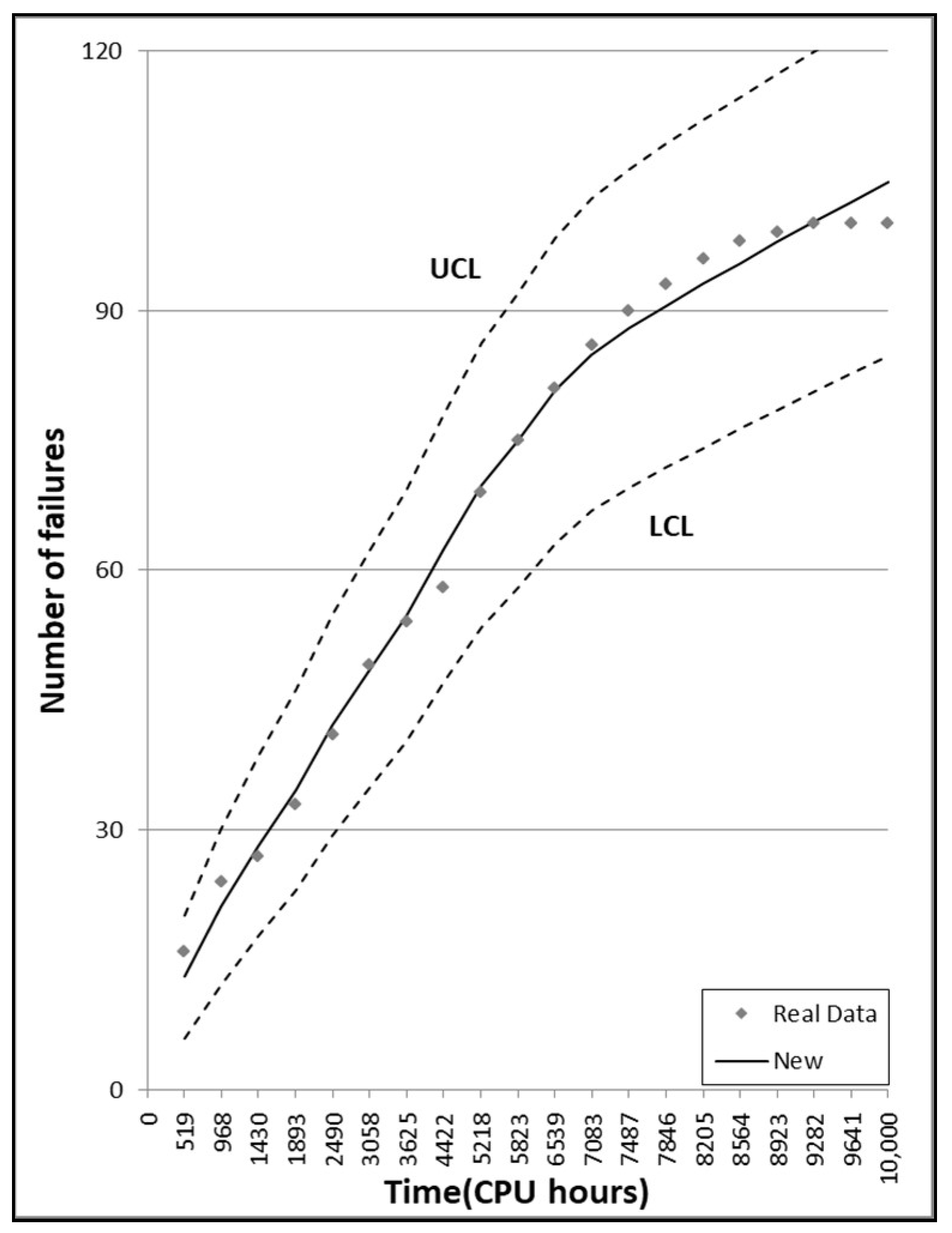
| Model | Time Index | 519 | 968 | 1430 | 1893 | 2490 | 3058 | 3625 | 4422 | 5218 | 5823 | |
| GOM | LCL | 3.641 | 9.407 | 15.376 | 21.176 | 28.274 | 34.589 | 40.464 | 48.022 | 54.803 | 59.482 | |
| 9.767 | 17.639 | 25.218 | 32.318 | 40.791 | 48.196 | 55.000 | 63.660 | 71.359 | 76.641 | |||
| UCL | 15.892 | 25.870 | 35.060 | 43.460 | 53.309 | 61.803 | 69.535 | 79.298 | 87.916 | 93.799 | ||
| DSM | LCL | −0.409 | 3.059 | 8.744 | 15.540 | 24.802 | 33.366 | 41.233 | 50.791 | 58.514 | 63.256 | |
| 2.966 | 8.910 | 16.770 | 25.422 | 36.671 | 46.770 | 55.885 | 66.811 | 75.550 | 80.883 | |||
| UCL | 6.342 | 14.760 | 24.796 | 35.305 | 48.540 | 60.174 | 70.537 | 82.832 | 92.586 | 98.510 | ||
| ISM | LCL | 3.641 | 9.407 | 15.376 | 21.176 | 28.273 | 34.589 | 40.464 | 48.022 | 54.802 | 59.482 | |
| 9.767 | 17.639 | 25.218 | 32.318 | 40.791 | 48.196 | 55.000 | 63.660 | 71.359 | 76.641 | |||
| UCL | 15.892 | 25.870 | 35.060 | 43.460 | 53.309 | 61.803 | 69.535 | 79.298 | 87.916 | 93.799 | ||
| YIDM | LCL | 3.631 | 9.384 | 15.337 | 21.122 | 28.202 | 34.503 | 40.367 | 47.916 | 54.698 | 59.387 | |
| 9.751 | 17.608 | 25.171 | 32.254 | 40.707 | 48.096 | 54.888 | 63.539 | 71.241 | 76.534 | |||
| UCL | 15.871 | 25.832 | 35.004 | 43.385 | 53.213 | 61.689 | 69.409 | 79.162 | 87.784 | 93.680 | ||
| PNZM | LCL | 3.701 | 9.506 | 15.493 | 21.294 | 28.373 | 34.657 | 40.493 | 47.993 | 54.724 | 59.378 | |
| 9.853 | 17.767 | 25.363 | 32.460 | 40.909 | 48.275 | 55.033 | 63.627 | 71.271 | 76.523 | |||
| UCL | 16.005 | 26.028 | 35.234 | 43.627 | 53.445 | 61.893 | 69.573 | 79.261 | 87.817 | 93.668 | ||
| PZM | LCL | 3.458 | 9.130 | 15.085 | 20.933 | 28.150 | 34.608 | 40.627 | 48.354 | 55.238 | 59.940 | |
| 9.499 | 17.277 | 24.856 | 32.024 | 40.646 | 48.218 | 55.187 | 64.039 | 71.852 | 77.157 | |||
| UCL | 15.539 | 25.424 | 34.628 | 43.116 | 53.141 | 61.828 | 69.747 | 79.723 | 88.466 | 94.373 | ||
| DPM | LCL | 26.407 | 26.678 | 27.161 | 27.873 | 29.166 | 30.827 | 32.943 | 36.756 | 41.628 | 46.096 | |
| 38.581 | 38.903 | 39.475 | 40.318 | 41.845 | 43.799 | 46.275 | 50.713 | 56.340 | 61.461 | |||
| UCL | 50.754 | 51.128 | 51.789 | 52.763 | 54.523 | 56.770 | 59.608 | 64.671 | 71.051 | 76.827 | ||
| TCM | LCL | 5.929 | 11.851 | 17.436 | 22.634 | 28.871 | 34.406 | 39.605 | 46.448 | 52.816 | 57.386 | |
| 12.993 | 20.787 | 27.763 | 34.075 | 41.497 | 47.982 | 54.009 | 61.863 | 69.110 | 74.278 | |||
| UCL | 20.058 | 29.723 | 38.090 | 45.516 | 54.122 | 61.559 | 68.413 | 77.279 | 85.404 | 91.170 | ||
| 3PFDM | LCL | 3.990 | 9.962 | 16.016 | 21.804 | 28.789 | 34.941 | 40.631 | 47.938 | 54.522 | 59.105 | |
| 10.271 | 18.361 | 26.012 | 33.076 | 41.400 | 48.605 | 55.191 | 63.564 | 71.041 | 76.216 | |||
| UCL | 16.552 | 26.759 | 36.008 | 44.348 | 54.011 | 62.270 | 69.752 | 79.190 | 87.561 | 93.327 | ||
| New | LCL | 5.981 | 12.096 | 17.800 | 23.076 | 29.375 | 34.946 | 40.168 | 47.027 | 53.403 | 57.974 | |
| 13.066 | 21.099 | 28.210 | 34.606 | 42.091 | 48.611 | 54.658 | 62.525 | 69.774 | 74.941 | |||
| UCL | 20.151 | 30.102 | 38.621 | 46.135 | 54.807 | 62.276 | 69.148 | 78.023 | 86.146 | 91.909 | ||
| Model | Time index | 6539 | 7083 | 7487 | 7846 | 8205 | 8564 | 8923 | 9282 | 9641 | 10,000 | |
| GOM | LCL | 64.535 | 68.049 | 70.489 | 72.543 | 74.495 | 76.350 | 78.112 | 79.786 | 81.376 | 82.886 | |
| 82.318 | 86.251 | 88.977 | 91.267 | 93.441 | 95.504 | 97.461 | 99.319 | 101.081 | 102.754 | |||
| UCL | 100.101 | 104.454 | 107.465 | 109.992 | 112.387 | 114.658 | 116.810 | 118.851 | 120.786 | 122.621 | ||
| DSM | LCL | 67.773 | 70.526 | 72.248 | 73.576 | 74.736 | 75.748 | 76.627 | 77.391 | 78.053 | 78.626 | |
| 85.943 | 89.018 | 90.939 | 92.418 | 93.710 | 94.834 | 95.812 | 96.660 | 97.395 | 98.031 | |||
| UCL | 104.112 | 107.510 | 109.629 | 111.260 | 112.683 | 113.921 | 114.997 | 115.930 | 116.738 | 117.437 | ||
| ISM | LCL | 64.535 | 68.049 | 70.489 | 72.543 | 74.495 | 76.350 | 78.112 | 79.786 | 81.376 | 82.886 | |
| 82.318 | 86.251 | 88.977 | 91.267 | 93.441 | 95.504 | 97.461 | 99.319 | 101.081 | 102.754 | |||
| UCL | 100.100 | 104.454 | 107.465 | 109.992 | 112.387 | 114.658 | 116.810 | 118.851 | 120.786 | 122.621 | ||
| YIDM | LCL | 64.460 | 67.996 | 70.457 | 72.532 | 74.508 | 76.389 | 78.181 | 79.887 | 81.511 | 83.059 | |
| 82.234 | 86.192 | 88.941 | 91.255 | 93.455 | 95.547 | 97.537 | 99.430 | 101.231 | 102.945 | |||
| UCL | 100.007 | 104.388 | 107.425 | 109.978 | 112.403 | 114.706 | 116.894 | 118.974 | 120.951 | 122.831 | ||
| PNZM | LCL | 64.417 | 67.936 | 70.389 | 72.462 | 74.440 | 76.328 | 78.131 | 79.854 | 81.500 | 83.074 | |
| 82.186 | 86.125 | 88.865 | 91.177 | 93.380 | 95.480 | 97.483 | 99.394 | 101.218 | 102.962 | |||
| UCL | 99.954 | 104.314 | 107.342 | 109.892 | 112.320 | 114.631 | 116.834 | 118.934 | 120.937 | 122.850 | ||
| PZM | LCL | 64.953 | 68.387 | 70.742 | 72.704 | 74.547 | 76.279 | 77.905 | 79.430 | 80.860 | 82.201 | |
| 82.786 | 86.629 | 89.260 | 91.447 | 93.499 | 95.425 | 97.231 | 98.924 | 100.510 | 101.995 | |||
| UCL | 100.619 | 104.872 | 107.777 | 110.189 | 112.451 | 114.571 | 116.558 | 118.418 | 120.160 | 121.789 | ||
| DPM | LCL | 52.288 | 57.681 | 62.083 | 66.287 | 70.771 | 75.541 | 80.600 | 85.954 | 91.607 | 97.562 | |
| 68.511 | 74.610 | 79.566 | 84.280 | 89.292 | 94.604 | 100.222 | 106.148 | 112.385 | 118.937 | |||
| UCL | 84.734 | 91.540 | 97.049 | 102.274 | 107.812 | 113.668 | 119.843 | 126.341 | 133.163 | 140.312 | ||
| TCM | LCL | 62.528 | 66.257 | 68.936 | 71.255 | 73.519 | 75.730 | 77.891 | 80.003 | 82.069 | 84.090 | |
| 80.065 | 84.247 | 87.243 | 89.832 | 92.355 | 94.815 | 97.216 | 99.560 | 101.849 | 104.086 | |||
| UCL | 97.603 | 102.237 | 105.550 | 108.408 | 111.190 | 113.900 | 116.541 | 119.116 | 121.629 | 124.082 | ||
| 3PFDM | LCL | 64.115 | 67.651 | 70.138 | 72.257 | 74.295 | 76.256 | 78.144 | 79.963 | 81.717 | 83.410 | |
| 81.847 | 85.806 | 88.586 | 90.949 | 93.218 | 95.399 | 97.497 | 99.515 | 101.459 | 103.333 | |||
| UCL | 99.578 | 103.961 | 107.033 | 109.641 | 112.142 | 114.543 | 116.849 | 119.067 | 121.202 | 123.257 | ||
| New | LCL | 63.115 | 66.844 | 69.522 | 71.840 | 74.104 | 76.315 | 78.476 | 80.590 | 82.657 | 84.680 | |
| 80.725 | 84.903 | 87.897 | 90.484 | 93.006 | 95.465 | 97.866 | 100.210 | 102.500 | 104.739 | |||
| UCL | 98.334 | 102.963 | 106.272 | 109.128 | 111.907 | 114.615 | 117.255 | 119.830 | 122.343 | 124.797 | ||
References
- Pham, T.; Pham, H. A generalized software reliability model with stochastic fault-detection rate. Ann. Oper. Res. 2017, 1–11. [Google Scholar] [CrossRef]
- Teng, X.; Pham, H. A new methodology for predicting software reliability in the random field environments. IEEE Trans. Reliab. 2006, 55, 458–468. [Google Scholar] [CrossRef]
- Pham, H. A new software reliability model with Vtub-Shaped fault detection rate and the uncertainty of operating environments. Optimization 2014, 63, 1481–1490. [Google Scholar] [CrossRef]
- Chang, I.H.; Pham, H.; Lee, S.W.; Song, K.Y. A testing-coverage software reliability model with the uncertainty of operation environments. Int. J. Syst. Sci. Oper. Logist. 2014, 1, 220–227. [Google Scholar]
- Inoue, S.; Ikeda, J.; Yamada, S. Bivariate change-point modeling for software reliability assessment with uncertainty of testing-environment factor. Ann. Oper. Res. 2016, 244, 209–220. [Google Scholar] [CrossRef]
- Okamura, H.; Dohi, T. Phase-type software reliability model: Parameter estimation algorithms with grouped data. Ann. Oper. Res. 2016, 244, 177–208. [Google Scholar] [CrossRef]
- Song, K.Y.; Chang, I.H.; Pham, H. A Three-parameter fault-detection software reliability model with the uncertainty of operating environments. J. Syst. Sci. Syst. Eng. 2017, 26, 121–132. [Google Scholar] [CrossRef]
- Song, K.Y.; Chang, I.H.; Pham, H. A software reliability model with a Weibull fault detection rate function subject to operating environments. Appl. Sci. 2017, 7, 983. [Google Scholar] [CrossRef]
- Li, Q.; Pham, H. NHPP software reliability model considering the uncertainty of operating environments with imperfect debugging and testing coverage. Appl. Math. Model. 2017, 51, 68–85. [Google Scholar] [CrossRef]
- Pham, H.; Nordmann, L.; Zhang, X. A general imperfect software debugging model with S-shaped fault detection rate. IEEE Trans. Reliab. 1999, 48, 169–175. [Google Scholar] [CrossRef]
- Pham, H. A generalized fault-detection software reliability model subject to random operating environments. Vietnam J. Comput. Sci. 2016, 3, 145–150. [Google Scholar] [CrossRef]
- Akaike, H. A new look at statistical model identification. IEEE Trans. Autom. Control 1974, 19, 716–719. [Google Scholar] [CrossRef]
- Pham, H. System Software Reliability; Springer: London, UK, 2006. [Google Scholar]
- Goel, A.L.; Okumoto, K. Time dependent error detection rate model for software reliability and other performance measures. IEEE Trans. Reliab. 1979, 28, 206–211. [Google Scholar] [CrossRef]
- Yamada, S.; Ohba, M.; Osaki, S. S-shaped reliability growth modeling for software fault detection. IEEE Trans. Reliab. 1983, 32, 475–484. [Google Scholar] [CrossRef]
- Ohba, M. Inflexion S-shaped software reliability growth models. In Stochastic Models in Reliability Theory; Osaki, S., Hatoyama, Y., Eds.; Springer: Berlin, Germany, 1984; pp. 144–162. [Google Scholar]
- Yamada, S.; Tokuno, K.; Osaki, S. Imperfect debugging models with fault introduction rate for software reliability assessment. Int. J. Syst. Sci. 1992, 23, 2241–2252. [Google Scholar] [CrossRef]
- Pham, H.; Zhang, X. An NHPP software reliability models and its comparison. Int. J. Reliab. Qual. Saf. Eng. 1997, 4, 269–282. [Google Scholar] [CrossRef]
- Pham, H. Software Reliability Models with Time Dependent Hazard Function Based on Bayesian Approach. Int. J. Autom. Comput. 2007, 4, 325–328. [Google Scholar] [CrossRef]
- Li, X.; Xie, M.; Ng, S.H. Sensitivity analysis of release time of software reliability models incorporating testing effort with multiple change-points. Appl. Math. Model. 2010, 34, 3560–3570. [Google Scholar] [CrossRef]
- Pham, H. Software reliability and cost models: Perspectives, comparison, and practice. Eur. J. Oper. Res. 2003, 149, 475–489. [Google Scholar] [CrossRef]
- Pham, H.; Zhang, X. NHPP software reliability and cost models with testing coverage. Eur. J. Oper. Res. 2003, 145, 443–454. [Google Scholar] [CrossRef]
- Kimura, M.; Toyota, T.; Yamada, S. Economic analysis of software release problems with warranty cost and reliability requirement. Reliab. Eng. Syst. Saf. 1999, 66, 49–55. [Google Scholar] [CrossRef]
- Sgarbossa, F.; Pham, H. A cost analysis of systems subject to random field environments and reliability. IEEE Trans. Syst. Man Cybern. Part C Appl. Rev. 2010, 40, 429–437. [Google Scholar] [CrossRef]
- Musa, J.D.; Iannino, A.; Okumoto, K. Software Reliability: Measurement, Prediction, and Application; McGraw-Hill: New York, NY, USA, 1987. [Google Scholar]
- Stringfellow, C.; Andrews, A.A. An empirical method for selecting software reliability growth models. Empir. Softw. Eng. 2002, 7, 319–343. [Google Scholar] [CrossRef]
- Wood, A. Predicting software reliability. IEEE Comput. Soc. 1996, 11, 69–77. [Google Scholar] [CrossRef]


| No. | Model | |
|---|---|---|
| 1 | GO Model [14] | |
| 2 | Delayed S-shaped Model [15] | |
| 3 | Inflection S-shaped Model [16] | |
| 4 | Yamada ImperfectDebugging Model [17] | |
| 5 | PNZ Model [10] | |
| 6 | PZ Model [18] | |
| 7 | Dependent Parameter Model [19] | |
| 8 | Testing Coverage Model [4] | |
| 9 | Three parameter Model [7] | |
| 10 | Proposed New Model |
| Hour Index | Failures | Cumulative Failures | Hour Index | Failures | Cumulative Failures |
|---|---|---|---|---|---|
| 1 | 27 | 27 | 14 | 5 | 111 |
| 2 | 16 | 43 | 15 | 5 | 116 |
| 3 | 11 | 54 | 16 | 6 | 122 |
| 4 | 10 | 64 | 17 | 0 | 122 |
| 5 | 11 | 75 | 18 | 5 | 127 |
| 6 | 7 | 83 | 19 | 1 | 128 |
| 7 | 2 | 84 | 20 | 1 | 129 |
| 8 | 5 | 89 | 21 | 2 | 131 |
| 9 | 3 | 92 | 22 | 1 | 132 |
| 10 | 1 | 93 | 23 | 2 | 134 |
| 11 | 4 | 97 | 24 | 1 | 135 |
| 12 | 7 | 104 | 25 | 1 | 136 |
| 13 | 2 | 106 | - | - | - |
| Week Index | Failures | Cumulative Failures | Week Index | Failures | Cumulative Failures |
|---|---|---|---|---|---|
| 1 | 90 | 90 | 10 | 0 | 190 |
| 2 | 17 | 107 | 11 | 2 | 192 |
| 3 | 19 | 126 | 12 | 0 | 192 |
| 4 | 19 | 145 | 13 | 0 | 192 |
| 5 | 26 | 171 | 14 | 0 | 192 |
| 6 | 17 | 188 | 15 | 11 | 203 |
| 7 | 1 | 189 | 16 | 0 | 203 |
| 8 | 1 | 190 | 17 | 1 | 204 |
| 9 | 0 | 190 | - | - | - |
| Time Index (CPU hours) | Cumulative Failures | Time Index (CPU hours) | Cumulative Failures | Time Index (CPU hours) | Cumulative Failures |
|---|---|---|---|---|---|
| 519 | 16 | 4422 | 58 | 8205 | 96 |
| 968 | 24 | 5218 | 69 | 8564 | 98 |
| 1430 | 27 | 5823 | 75 | 8923 | 99 |
| 1893 | 33 | 6539 | 81 | 9282 | 100 |
| 2490 | 41 | 7083 | 86 | 9641 | 100 |
| 3058 | 49 | 7487 | 90 | 10,000 | 100 |
| 3625 | 54 | 7846 | 93 | - | - |
| Model | LSE’s | MSE | AIC | PRR | PP | SAE | R2 |
|---|---|---|---|---|---|---|---|
| GOM | = 136.050, = 0.138 | 33.822 | 121.878 | 0.479 | 0.262 | 118.530 | 0.972 |
| DSM | = 124.665, = 0.356 | 134.582 | 210.287 | 12.787 | 1.181 | 239.335 | 0.889 |
| ISM | = 136.050, = 0.138 = 0.0001 | 35.363 | 123.878 | 0.479 | 0.262 | 118.532 | 0.972 |
| YIDM | = 81.252, = 0.340 = 0.0333 | 9.435 | 116.403 | 0.035 | 0.031 | 60.842 | 0.993 |
| PNZM | = 81.562, = 0.337 = 0.033, = 0.00 | 9.888 | 118.388 | 0.037 | 0.032 | 60.877 | 0.993 |
| PZM | = 0.01, = 0.138 = 800.0, = 0.00, = 136.04 | 38.895 | 127.878 | 0.479 | 0.262 | 118.530 | 0.972 |
| DPM | = 28650, = 0.003 = 0.00, = 71.8 | 274.911 | 382.143 | 0.857 | 3.568 | 304.212 | 0.792 |
| TCM | = 0.000035, = 0.734, = 0.29, = 0.002, = 427 | 7.640 | 116.932 | 0.019 | 0.019 | 47.304 | 0.995 |
| 3PFDM | = 1.696, = 0.001 = 6.808, = 1.574 = 173.030 | 17.827 | 119.523 | 0.137 | 0.100 | 81.313 | 0.987 |
| New Model | = 0.277, = 0.328 = 17.839, = 228.909 | 7.361 | 114.982 | 0.022 | 0.022 | 47.869 | 0.994 |
| Model | LSE’s | MSE | AIC | PRR | PP | SAE | R2 |
|---|---|---|---|---|---|---|---|
| GOM | = 197.387, = 0.399 | 80.678 | 184.331 | 0.170 | 0.101 | 104.403 | 0.939 |
| DSM | = 192.528, = 0.882 | 232.628 | 331.857 | 1.291 | 0.333 | 142.544 | 0.823 |
| ISM | = 197.354, = 0.399 = 0.000001 | 86.440 | 186.334 | 0.171 | 0.101 | 104.370 | 0.939 |
| YIDM | = 182.934, = 0.464 = 0.0071 | 78.837 | 157.825 | 0.128 | 0.087 | 100.617 | 0.944 |
| PNZM | = 183.124, = 0.463 = 0.007, = 0.00 | 84.902 | 159.873 | 0.128 | 0.087 | 100.608 | 0.944 |
| PZM | = 195.990, =0.3987 = 1000.00, = 0.00, = 1.390 | 100.989 | 190.332 | 0.172 | 0.102 | 104.354 | 0.939 |
| DPM | = 26124.0, = 0.0044 = 0.00, = 147.00 | 769.282 | 480.341 | 0.415 | 0.712 | 334.128 | 0.494 |
| TCM | = 0.053, = 0.774, = 181.0, = 38.6, = 204.1 | 72.283 | 158.933 | 0.052 | 0.048 | 103.196 | 0.956 |
| 3PFDM | = 0.028, = 0.210 = 9.924, = 0.005 = 206.387 | 81.090 | 163.797 | 0.073 | 0.061 | 106.341 | 0.951 |
| New Model | = 0.008, = 0.275, = 0.001, = 207.873 | 60.623 | 151.156 | 0.043 | 0.041 | 98.705 | 0.960 |
| Model | LSE’s | MSE | AIC | PRR | PP | SAE | R2 |
|---|---|---|---|---|---|---|---|
| GOM | = 133.835, = 0.000146 | 8.620 | 86.136 | 0.556 | 0.242 | 42.166 | 0.991 |
| DSM | = 101.918, = 0.000507 | 45.783 | 117.316 | 22.692 | 1.318 | 101.659 | 0.951 |
| ISM | = 133.835, = 0.000146 = 0.000001 | 9.127 | 88.136 | 0.556 | 0.242 | 42.166 | 0.991 |
| YIDM | = 130.091, = 0.00015 = 0.000003 | 9.084 | 88.267 | 0.561 | 0.243 | 42.052 | 0.991 |
| PNZM | = 121.178, = 0.000163 = 0.000009, = 0.00 | 9.532 | 90.326 | 0.530 | 0.234 | 41.538 | 0.991 |
| PZM | = 122.259, = 0.0002 = 9955.597, = 0.305 = 0.569 | 11.491 | 92.020 | 0.643 | 0.268 | 44.848 | 0.990 |
| DPM | = 123.193, = 0.0001 = 0.0001, = 38.459 | 156.480 | 212.867 | 0.917 | 2.879 | 196.360 | 0.851 |
| TCM | = 0.000013, = 0.78, = 141.399, = 54.71, = 254.707 | 7.090 | 90.758 | 0.091 | 0.068 | 37.880 | 0.9937 |
| 3PFDM | = 0.016, = 0.07 = 0.00001, = 157.458 = 205.025 | 9.410 | 92.360 | 0.420 | 0.200 | 39.909 | 0.992 |
| New Model | = 0.064, = 0.731, = 2509.898, = 337.765 | 6.336 | 88.885 | 0.086 | 0.066 | 36.250 | 0.9940 |
| Warrnaty Period | C1(T) | T* | C2(T) | T* | C3(T) | T* |
|---|---|---|---|---|---|---|
| Tw = 2 | 1173.41 | 14.2 | 1403.78 | 11.6 | 599.88 | 10.5 |
| Tw = 5 | 1286.95 | 14.9 | 1928.63 | 22.8 | 1334.72 | 11.3 |
| Tw = 10(basic) | 1338.70 | 15.1 | 2398.24 | 34.7 | 2263.33 | 12.3 |
| Tw = 15 | 1348.88 | 15.2 | 2702.33 | 42.7 | 2969.88 | 13.0 |
| Cost Coefficient C2 | C1(T) | T* | C2(T) | T* | C3(T) | T* |
|---|---|---|---|---|---|---|
| C2 = 25 | 1036.02 | 15.2 | 2013.25 | 37.5 | 1972.06 | 12.5 |
| C2 = 50 (basic) | 1338.70 | 15.1 | 2398.24 | 34.7 | 2263.33 | 12.3 |
| C2 = 100 | 1943.64 | 15.1 | 3141.20 | 29.1 | 2843.35 | 12.1 |
| Cost Coefficient C3 | C1(T) | T* | C2(T) | T* | C3(T) | T* |
|---|---|---|---|---|---|---|
| C3 = 500 | 1270.65 | 16.5 | 2398.24 | 34.7 | 2262.96 | 12.4 |
| C3 = 2000 (basic) | 1338.70 | 15.1 | 2398.24 | 34.7 | 2263.33 | 12.3 |
| C3 = 4000 | 1376.26 | 14.6 | 2398.24 | 34.7 | 2263.77 | 12.3 |
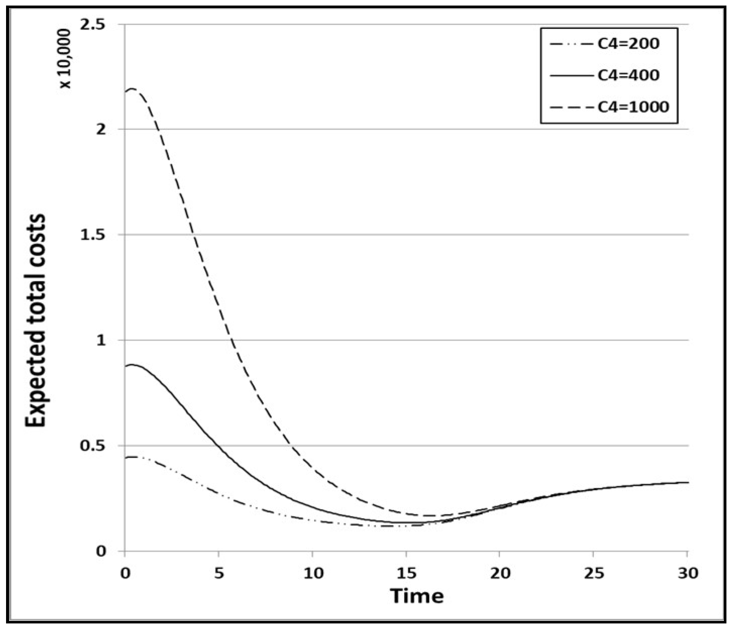
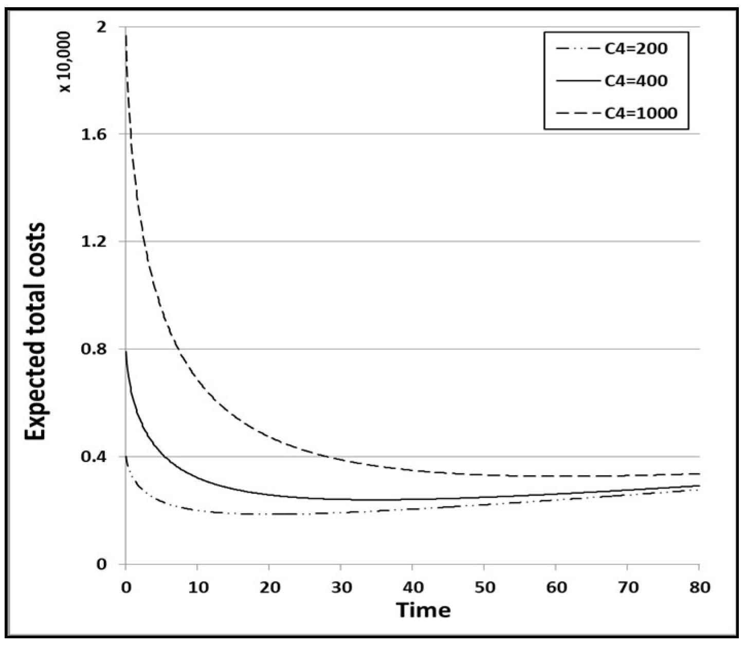
| Cost Coefficient C4 | C1(T) | T* | C2(T) | T* | C3(T) | T* |
|---|---|---|---|---|---|---|
| C4 = 200 | 1183.14 | 14.3 | 1859.29 | 20 | 1590.02 | 11.6 |
| C4 = 400 (basic) | 1338.70 | 15.1 | 2398.24 | 34.7 | 2263.33 | 12.3 |
| C4 = 1000 | 1680.99 | 16.3 | 3272.23 | 61 | 4253.45 | 12.8 |
© 2017 by the authors. Licensee MDPI, Basel, Switzerland. This article is an open access article distributed under the terms and conditions of the Creative Commons Attribution (CC BY) license (http://creativecommons.org/licenses/by/4.0/).
Share and Cite
Song, K.Y.; Chang, I.H.; Pham, H. An NHPP Software Reliability Model with S-Shaped Growth Curve Subject to Random Operating Environments and Optimal Release Time. Appl. Sci. 2017, 7, 1304. https://0-doi-org.brum.beds.ac.uk/10.3390/app7121304
Song KY, Chang IH, Pham H. An NHPP Software Reliability Model with S-Shaped Growth Curve Subject to Random Operating Environments and Optimal Release Time. Applied Sciences. 2017; 7(12):1304. https://0-doi-org.brum.beds.ac.uk/10.3390/app7121304
Chicago/Turabian StyleSong, Kwang Yoon, In Hong Chang, and Hoang Pham. 2017. "An NHPP Software Reliability Model with S-Shaped Growth Curve Subject to Random Operating Environments and Optimal Release Time" Applied Sciences 7, no. 12: 1304. https://0-doi-org.brum.beds.ac.uk/10.3390/app7121304