Recognition Algorithm Based on Improved FCM and Rough Sets for Meibomian Gland Morphology

Abstract

To overcome the limitation of artificial judgment of meibomian gland morphology, we proposed a solution based on an improved fuzzy c-means (FCM) algorithm and rough sets theory. The rough sets reduced the redundant attributes while ensuring classification accuracy, and greatly reduced the amount of computation to achieve information dimension compression and knowledge system simplification. However, before this reduction, data must be discretized, and this process causes some degree of information loss. Therefore, to maintain the integrity of the information, we used the improved FCM to make attributes fuzzy instead of discrete before continuing with attribute reduction, and thus, the implicit knowledge and decision rules were more accurate. Our algorithm overcame the defects of the traditional FCM algorithm, which is sensitive to outliers and easily falls into local optima. Our experimental results show that the proposed method improved recognition efficiency without degrading recognition accuracy, which was as high as 97.5%. Furthermore, the meibomian gland morphology was diagnosed efficiently, and thus this method can provide practical application values for the recognition of meibomian gland morphology.

1. Introduction

In recent years, a variety of new medical devices have been used to help doctors with clinical diagnosis while producing a large amount of image data. Manual interpretation of images relies too much on physician experience and is not very efficient. To this end, many scholars attempt to use computer-assisted processing of medical images. In the work by Xu et al. [1], the support vector machine was used to recognize brain magnetic resonance imaging (MRI) images with a recognition rate up to 95.45%. In another study, overcoming the influence of fracture diversity and individual differences, a decision tree was used to achieve automatic X-detection [2]. The method by Tang et al. [3] used fuzzy recognition to classify white blood cell images to solve the contradiction between real-time detection accuracy and speed. Chen et al. [4] developed a new method for the filtering of X-ray digital images of chests based on multi-resolution and rough set. This paper attempts to use image recognition technology to assist doctors in interpreting meibomian gland images and thus improve diagnostic accuracy and efficiency.

Meibomian gland dysfunction (MGD) is a very common eye disease [5]. In recent years, with the increase of electronic products, the incidence of MGD has increased dramatically, seriously affecting people’s normal lives. Many experts have conducted numerous research studies on MGD in order to determine how to prevent the disease, offer timely diagnosis, and reduce the troubles caused by the disease. However, the current recognition of meibomian gland morphology still relies on the experience of doctors. With the development of pattern recognition technologies and continuous improvement of clinical diagnostic requirements, it is necessary to develop an intelligent diagnosis system that can replace human experience with advanced science and technology.

The rough sets theory was proposed in 1982 by Z. Pawlak [6], a Polish mathematician, whose main idea was to improve the accuracy and correctness of data analysis through attribute reduction under the premise of keeping the same classification ability. However, continuous attributes must be discretized before using rough sets theory to do attribute reduction for information system, and this process results in some degree of information loss. The fuzzy rough sets theory, presented by French scholars Dubois and Prade [7], combines the advantages of fuzzy sets and rough sets, and extends precise sets to fuzzy sets, and fuzzy equivalence classes are determined by the membership function, thus avoiding information loss to a certain extent. Rough sets theory has been developed in theoretical research and applied research for more than thirty years. Currently, many scholars apply rough sets theory to industrial control [8,9,10], agricultural science [11,12], aerospace, military applications, and other fields [13,14]. However, the application of fuzzy rough sets is not commonly used in medical image recognition, and available literature is relatively lacking. Moreover, compared with other image recognition technologies, fuzzy rough sets theory is more suitable for processing medical images with intense ambiguity and uncertainty [15].

In this paper, we propose a diagnostic algorithm based on a modified fuzzy c-means (FCM) algorithm and rough sets for the recognition of meibomian gland morphology. The FCM algorithm is one of the most widely used clustering algorithms due to its simple and fast convergence and its ability to handle large datasets [16]. In this paper, the defects of the traditional FCM algorithm are improved, such as the random selecting of the initial clustering center and the algorithm’s sensitivity to isolated points. The improved FCM was used to cluster the data to obtain the fuzzy division of meibomian gland morphological parameters, thus avoiding information loss [17]. Subsequently, the rough sets theory was used to process the data in order to eliminate redundant samples and attributes. The compression of the information dimension and the simplification of knowledge system were also realized, and the most effective classification rule was extracted. The proposed algorithm improved recognition rate without reducing accuracy, and realized high efficiency diagnosis of meibomian gland morphology.

2. Materials and Methods

2.1. Basic Concepts of the Rough Sets Theory

Based on the classification mechanism, the rough sets theory’s research object is the information system [18]. By introducing an indiscernibility relation as the theoretical basis, and defining the concepts of upper and lower approximations, the rough sets theory focuses on knowledge reduction and determining attribute importance. Through attribute reduction, the fuzziness and uncertainty knowledge can be described by the knowledge in the existing knowledge base.

2.1.1. Indiscernibility Relation

We defined the domain $U$ as a non-empty finite set of the samples we are interested in, and any subset $X$ which satisfies the condition $X\subseteq U$ can be called a concept or a category in $U$. Furthermore, any concept set of $U$ can be called basic knowledge of $U$, which represents the individual classification in the domain $U$, referred to as $U$’s knowledge. Let $R$ be an equivalence relation on $U$, $U/R$ denotes all equivalence classes, and ${[x]}_R$ represents equivalent classes of $R$ that contain element $x$, which satisfies the condition $x\in U$. If $P\subseteq R$ and $P\ne \varnothing$, the intersection of all equivalence relations in $P$ is also an equivalence relation, and this equivalence relation is called $P$-indiscernibility relation, denoted as $ind(P)$. In the process of classification, the individuals with little difference are classified into the same classification, and their relationship is an indiscernibility relation, which is equivalent to an equivalence relation on $U$.

The concept of indiscernibility relation is the cornerstone of the rough sets theory, which reveals the granular structure of domain knowledge. The concept assumes that some knowledge is in the domain, and uses attributes and attributes’ values to describe the objects. If two objects have the same attributes and attributes’ values, they have an indiscernibility relation. Mathematically, the indiscernibility relation of a set and the division of a set are equivalent concepts, one-to-one, and unique to each other. This concept means that objects in the domain can be described with different attributes’ sets to express exactly the same facts.

2.1.2. Lower and Upper Approximations

Let $X$ denote the subset of elements of the domain $U$ ($X\subseteq U$ and $X\ne \varnothing$), and $R$ denote an equivalence relation on $U$. The lower approximation of $X$ in $R$, denoted as $\underset{\_}{R}X$, is defined as the union of all these elementary sets contained in $X$. More formally,

$$\underset{\_}{R}X=\cup \{Y\in U/R|Y\subseteq X\}.$$

The upper approximation of set $X$, denoted as $\overline{R}X$, is the union of these elementary sets, which have a non-empty intersection with $X$:

$$\overline{R}X=\cup \{Y\in U/R|Y\cap X\ne \varnothing \}.$$

In general, Figure 1 represents the upper approximation and lower approximation. The area in the black box is the domain $U$, the area in the green curve denotes $X$, the inner red curve denotes the upper approximation set $\overline{R}X$, and the blue curve denotes the lower approximation set $\underset{\_}{R}X$.

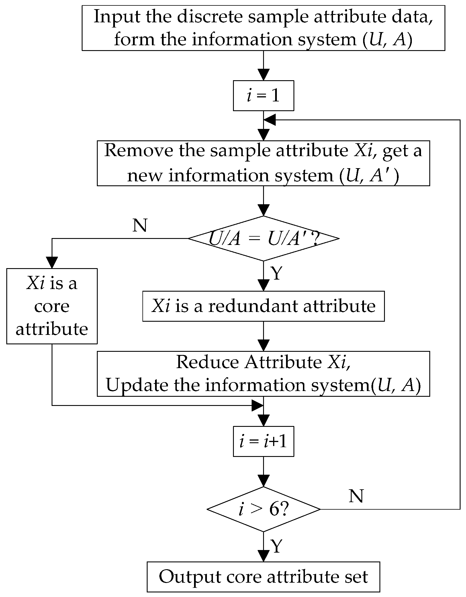
2.1.3. Core and Attribute Reduction

The concepts of core and attribute reduction are two fundamental concepts of the rough sets theory. The attribute reduction is the essential part of an information system, which can discern all dispensable objects from the original information system. The core is the basis of attribute reduction. The information system may not have only one reduction, the intersection of all reductions is called the core of the information system.

Let $P$ be a set of equivalence relations, and $P\subseteq R$ and $P\ne \varnothing$. If $ind(R)=ind(R-P)$, then the set $P$ can be dispensed in the set $R$, otherwise it cannot be dispensed. If each $P$ in the set $R$ is not dispensable, $P$ is independent, otherwise it is dependent. If the set of condition attributes is independent, one may be interested in finding all possible minimal subset of attributes and the set of all indispensable attributes (core).

Given an information system $S=(U,A)$, in which $U$ is a non-empty finite set and $A=C\cup D$ and $C\cap D\ne \varnothing$, $C$ indicates the set of the condition attributes, and $D$ indicates the set of decision attributes. If $B\subseteq C$ and $d\subseteq D$, $pos(d)=\cup \{\underset{\_}{B}(X)|X\in U/ind(d)\}$ is the relative positive region of the decision attribute $d$ with respect to $B$.

Let $P$ and $Q$ be equivalence relationship sets. If $po{s}_{ind(P)}(ind(Q))=po{s}_{ind(P-\{R\})}(ind(Q))$, then $R$ can be reduced by $P$. The set of all irreducible equivalence relationships of $Q$ in $P$ is called the core of $P$, and is denoted as $cor{e}_Q(P)$. Core is the set containing the most important attributes for classification in the condition attributes, and without them, the quality of the classification will drop.

The relation between the reduction of attributes’ set and the core is as follows:

$$core\left(P\right)=\cap red\left(P\right)$$

The expression $red\left(P\right)$ represents all the reductions of $P$. The expression $core\left(P\right)$ contains all the equivalence relations in the reduction of $P$, which is the important and indispensable attributes’ set in $P$.

The concept of $core\left(P\right)$ has two meanings:

(1)

the $core\left(P\right)$ is used as the basis for the calculation of attribute reduction.

(2)

the $core\left(P\right)$ is a feature set that cannot be eliminated in attribute reduction.

The concept of $core\left(P\right)$ provides a powerful mathematical tool for extracting important attributes and their values from the condition attributes by attribute reduction. The attributes in the set of condition attributes are not equally important, even some of them are redundant. The processing of attribute reduction aims to reduce the unnecessary condition attributes or remove redundant attributes in the information system, and obtain the smallest set of condition attributes that can ensure correct classification. In other words, the classification quality of the reduced attributes’ set is the same as that of the original attributes’ set. Under the condition of guaranteeing the classification ability of the information system, attribute reduction can get a simpler and more effective decision rule. Lastly, attribute reduction is not only the approach and method of obtaining classified knowledge from an information system, but also the focus and essence of the rough sets theory research.

2.2. FCM

The FCM clustering algorithm is a fuzzy recognition unsupervised algorithm based on the division of clustering algorithm. It only provides the number of clusters, and constantly modifies the sample type, cluster centers, and membership of each sample belonging to various categories, and ultimately achieves an objective function with a best classification.

2.2.1. Traditional FCM Algorithm

Let $X=\{x_1,x_2,\cdots ,x_n\}$ be a dataset containing $n$ samples, $v_i(i=1,2,\cdots ,c)$ is the center of each cluster, $c$ is the number of clusters, and ${\mu }_{ik}$ is the membership of the sample $k$ belonging to the class $i$. Dunn [19] defined the objective function as follows:

$$J(X;U,V)={\displaystyle \sum _{i=1}^c{\displaystyle \sum _{k=1}^n{({\mu }_{ik})}^m\left|\right|x_k-v_i|{|}_A^2}}$$

where $U$ is the membership matrix, $V$ is the matrix of cluster centers; $D_{ikA}^2=\left|\right|x_k-v_i|{|}_A^2={(x_k-v_i)}^{T}A(x_k-v_i)$ is the Euclidean distance from samples to the cluster centers; $A$ is a positive definite matrix; and $m$ is a weighted index affecting the degree of fuzzy membership matrix. Generally, $m$ is 2. The FCM clustering requires that membership meets the following condition:

$${\displaystyle \sum _{i=1}^c{\mu }_{ik}}=1,1\le k\le n$$

Using the Lagrange multiplier method [20,21], the condition of the objective function achieving the minimum is as follows:

$${\mu }_{ik}=\frac{1}{{\displaystyle {\sum }_{j=1}^c(D_{ikA}/D_{jkA}{)}^{2/(m-1)}}},1\le i\le c,1\le k\le n$$

$$v_i=\frac{{\displaystyle \sum _{k=1}^N{\mu }_{ik}^m{x}_k}}{{\displaystyle \sum _{k=1}^N{\mu }_{ik}^m}}$$

It can be seen that the FCM clustering algorithm obtains the cluster centers through the iteration of ${\mu }_{ik}$ and $v_i$.

2.2.2. Improved FCM Algorithm

The FCM algorithm is very simple and does not need to conduct large-scale operations because the establishment of the sample category’s fuzzy description can well reflect the objective world. However, when dealing with practical applications, there are still some problems [22].

First, the FCM algorithm must give the initial cluster center before clustering. Like most nonlinear optimization problems, the FCM clustering effect is directly affected by the initial value.

Second, the FCM algorithm has a good effect on data with strong regularity distribution. However, when the samples contain noise, the clustering center is shifted to the noise point, and even the noise will be selected as the cluster center, which seriously affects the clustering effect.

To solve these problems, we proposed a method for selecting the initial clustering center based on distance. Our clustering results were globally optimal. According to the Lazard’s criterion [23,24], the noise point in the data is defined as follows: the deviation between the point and the mean is more than twice the standard deviation of the samples. In this paper, we located the noise points according to the sample’s distance, and then dealt with them to make the algorithm insensitive to noise points.

Before introducing the improved algorithm, several related concepts are introduced as follows:

• Distances between samples (Euclidean distance):

  $$d(x_i,x_j)=\sqrt{|x_{i1}-y_{j1}{|}^2+|x_{i2}-y_{j2}{|}^2+\cdots +|x_{im}-y_{jm}{|}^2}$$
• The mean of the distances of sample $x_i$ to other samples:

  $$m_i=\frac{1}{n}{\displaystyle \sum _{j=1}^{n}d(x_i,x_j)}$$
• The mean of the distances of all samples:

  $$d=\frac{2}{n(n+1)}{\displaystyle \sum _{i=1}^n{\displaystyle \sum _{j=1}^{i}d(x_i,x_j)}}$$
• Noise point:

In the dataset $X$, if the sample point $x_i$ satisfies $m_i>2d$, we call $x_i$ the noise point.

$X=\{x_1,x_2,\cdots ,x_n\}$ is the set of classified samples, and the set of the number of clusters is $c$. Selecting the initial cluster center in the improved algorithm was performed as follows:

Step 1:

Calculate the mean distance $m_i$ from sample $x_i$ to other samples, generate the sample distance vector, and take the sample point with the smallest mean distance as the first cluster center;

Step 2:

Calculate the mean of the distances of all samples $d$, mark the sample point $x_i$, which satisfies $m_i>2d$ as the noise point, and put the noise point into a separate set;

Step 3:

Use the distance vector to determine the non-isolated samples whose distance from the first clustering center is larger than $d$, and choose the second cluster center with the smallest mean distance from the first center from among these samples.

Step 4:

Repeat step 3 until $c$ cluster centers are found.

Step 5:

According to the distance, classify the noise points to the corresponding classification.

The operation flow of the improved FCM algorithm is shown in Figure 2.

2.2.3. Results Analysis of the Improved FCM Algorithm

To verify the effectiveness of the proposed algorithm, the traditional FCM algorithm and the improved version were used to cluster datasets with noise. Figure 3 shows the effect of the two kinds of clustering methods on processing the datasets, where “ο”, “Δ”, and “+” represent different categories, and “♢” indicates the cluster center of each class. It can be seen that the clustering results were seriously affected by noise and the clustering centers were deviated using the traditional FCM algorithm. After the improved FCM was used to remove the isolated points, the clustering results became more reasonable.

Table 1. Clustering effect comparison between the traditional FCM algorithm and the improved FCM algorithm.

Algorithm Category	Clustering Center	Number of Iterations	Objective Function
traditional FCM algorithm	(16.32,70.00), (60.96,23.88), (39.98,86.77)	31	3.49 × 104
improved FCM algorithm	(16.07,63.25), (42.24,86.78), (20.02,82.18)	16	1.95 × 104

shows the results of the two clustering algorithms. It can be seen that the traditional FCM was sensitive to noise and easily trapped in the local optima. Conversely, through selecting a reasonable initial clustering center and removing the influence of isolated points, the improved FCM reduced the number of iterations while clustering correctly and improving the final objective function.

3. MGD Identification Based on Improved FCM and Rough Sets

Different morphologies of the meibomian gland show different texture features in images. Figure 4 shows four typical kinds of meibomian glands. Figure 4a shows a normal type, the distribution of the gland ducts is uniform, and there is no expansion or deletion of the gland ducts; Figure 4b shows a shortened type, and ductal arrangement is neat, shortened, and the loss area of the gland ducts is less than one third of the total area; Figure 4c shows a deletion type, the loss of the gland ducts is obvious, and the loss area is one thirds to two thirds of the total area; Figure 4d shows a serious deletion type, the gland ducts are not obvious, and basically all of them are missing.

The methods used for meibomian gland image recognition usually include image preprocessing, feature extraction, classification, and decision-making. In this paper, we applied the improved FCM and rough sets theory to meibomian gland image recognition. The workflow chart is shown in Figure 5.

3.1. Image Preprocessing

The purpose of image preprocessing is to improve image quality by the corresponding image processing method, making it more suitable for both observation and judgment by human eyes, and the analysis and processing by computers. Generally, image preprocessing includes image enhancement and image segmentation.

3.1.1. Image Enhancement

Images of meibomian glands are often blurred due to the limitation of equipment and man-made operation. There is no obvious gray difference in some details, so the image quality is not high, thus affecting the doctor’s decision. Image enhancement improves quality and gray levels so that the enhanced details of the image are more suitable for human eyes or machine processing. In this paper, we used enhanced high-pass filter technology to eliminate ambiguity, inhibit low-frequency components, and enhance high-frequency components. These made images more clear. A Gaussian high-pass filter was used to filter the image, and the transfer function is shown as follows:

$$H(u,v)=1-{\mathrm{e}}^{-D^2(u,v)/2{\sigma }^2}$$

The edge and details of the filtered image were enhanced. However, since the high-pass filter deviated from the direct-current component, the average grayscale of the image was reduced to zero. To correct this, we used high-frequency emphasis filtering. The transfer function is as follows:

$$H_f(u,v)=a+bH(u,v)$$

where $H(u,v)$ is the transfer function of the high-pass filtering, Gaussian filter used herein; a denotes the offset; and b denotes the multiplier. When offset a is less than 1 and the high-frequency multiplier b is greater than 1, the low-frequency component is suppressed, and the high frequency component is enhanced. The enhanced images are shown in Figure 6. Experiments showed that this method was convenient and effective for the enhancement of meibomian gland images, achieving greater image quality that could aid in diagnosis.

3.1.2. Image Segmentation

Image segmentation segments the region of interest in the image to provide a reliable basis for subsequent analysis and processing [25]. Segmentation quality directly affects subsequent image recognition. The eyelid part is of great significance in the diagnosis of meibomian gland morphology. Using the differences of textures between the eyelid region and other regions, and combining morphological and local entropy filtering, we designed a segmentation method based on texture filtering. The local entropy is defined as an entropy operation on an area of $n\times n$ centered on the selected pixel, and the meibomian gland image was filtered using local entropy to obtain the texture image. Local entropy calculation expressions are shown as follows:

$$H=-{\displaystyle \sum _{i=1}^n{\displaystyle \sum _{j=1}^n{p}_{ij}}}\log p_{ij}$$

$$p_{ij}=f(i,j)/{\displaystyle \sum _i^n{\displaystyle \sum _j^{n}f(i,j)}}$$

where $f(i,j)$ denotes the local pixels of $n\times n$, and $p_{ij}$ is the probability that the current pixel gray level occupies the local total gray level. The larger the local entropy is, the smaller the texture difference is in the window. Therefore, threshold segmentation can be performed according to the local entropy of the image to extract the target region. Due to the limitation of the artificially defined threshold, the segmentation result may appear over-segmentation, holes or the boundary of segmented image may not be smooth or other phenomena may result. In this paper, we used a morphological method to smooth edges, and filled the empty holes to obtain high-quality segmentation images. As shown in Figure 7, our method accurately and effectively segmented meibomian gland images while ensuring image integrity. The details of the target area were all retained, which laid the foundation for follow-up treatment.

3.2. Tamura Texture Feature Extraction

According to human visual perception and the basis of psychological experiments, Tamura et al. [26,27] proposed a texture feature expression, containing coarseness, contrast, directionality, line-likeness, regularity, and roughness. In this paper, we studied the characteristics of texture features of meibomian gland images.

3.2.1. Coarseness

Coarseness, the most basic texture feature, reflects particle size. Coarseness can be calculated with the following steps:

First, calculate the average intensity of the pixels in the active window of size $2^k\times 2^k$ in the image, expressed as

$$A_k(x,y)={\displaystyle \sum _{i=x-2^{k-1}}^{x+2^{k-1}-1}{\displaystyle \sum _{j=y-2^{k-1}}^{y+2^{k-1}-1}g(i,j)/2^{2k}}}$$

where $k=0,1,\cdots ,5$, and $g(i,j)$ is the gray-level at $(i,j)$.

Then, separately calculate the average intensity difference between the windows of each pixel that do not overlap in the horizontal and vertical directions, respectively. This is expressed as follows:

$$E_h(x,y)=|A_k(x+2^{k-1},y)-A_k(x-2^{k-1},y)|$$

$$E_v(x,y)=|A_k(x,y+2^{k-1})-A_k(x,y-2^{k-1})|$$

For each pixel, $k$, which maximizes the value of $E$, is used to set the optimum size $S_{best}(x,y)=2^k$.

Finally, coarseness can be obtained by calculating the mean value of $S_{best}$ in the whole image, which is expressed as follows:

$$F_{crs}=\frac{1}{mn}{\displaystyle \sum _{i=1}^m{\displaystyle \sum _{j=1}^n{S}_{best}(i,j)}}$$

where $m$ and $n$ are the effective width and height of the image, respectively.

3.2.2. Contrast

Contrast is obtained by statistical analysis of pixel intensity distribution. Generally, the contrast feature is determined by the degree of grayscale dynamic range of the image and the degree of polarization between the black and white portions of the histogram. These two factors can be defined by the kurtosis ${\alpha }_4={\mu }_4/{\sigma }^4$, where ${\mu }_4$ is the fourth moment about the mean, and ${\sigma }^2$ which can measure the dispersion in the distribution, is the variance about the mean of the gray-levels probability distribution. Contrast can be defined as:

$$F_{con}=\frac{\sigma }{{\alpha }_4^{1/4}}$$

3.2.3. Directionality

The degree of direction is the global characteristics of a given texture region, and describes how textures are scattered or concentrated in some direction. First, calculate the direction of the gradient vector of each pixel. The mode and direction of the gradient vector are defined as follows:

$$|\Delta G|=(|{\Delta }_H|+|{\Delta }_V|)/2$$

$$\mathsf{\theta }={\tan }^{-1}({\Delta }_V/{\Delta }_H)+\pi /2$$

where ${\Delta }_H$ and ${\Delta }_V$ are the amount of change in the horizontal and vertical directions of the image, respectively. When the gradient vectors of all pixels are calculated, $\mathsf{\theta }$ can be expressed using the histogram value $H_D$. Finally, the overall direction of the image can be obtained by calculating the sharpness of the peaks in the histogram, which is expressed as follows:

$$F_{dir}={\displaystyle \sum _P^n{\displaystyle \sum _{\mathsf{\Phi }\in W}(\mathsf{\Phi }-{\mathsf{\Phi }}_P}}{)}^2{H}_D(\mathsf{\Phi })$$

where $P$ denotes the peaks in the histogram, and $n$ is the number of peaks. For a given peak, $W$ represents all the discrete regions contained in the peak, and ${\mathsf{\Phi }}_P$ is the center of the peak.

3.2.4. Line-Likeness

Line-likeness is defined as the degree of coincidence of the co-occurrence matrix of directions of each pixel point. When calculating the co-occurrence matrix, the pixel pitch is denoted as $d$.

$$F_{lin}=\frac{{\displaystyle \sum _i^n{\displaystyle \sum _j^n{P}_{Dd}(i,j)\cos [(i-j)\frac{2\pi }{n}]}}}{{\displaystyle \sum _i^n{\displaystyle \sum _j^n{P}_{Dd}}}}$$

where $P_{Dd}$ is the distance point of the co-occurrence matrix of the local area $n\times n$.

3.2.5. Regularity

Since the texture characteristics of the whole image are not regular, the variance of partitioned sub-images is calculated. Four features of the sub-image are used to measure texture regularity, which is expressed as follows:

$$F_{reg}=1-r({\sigma }_{crs}+{\sigma }_{con}+{\sigma }_{dir}+{\sigma }_{lin})$$

where $r$ is a normalizing factor and ${\sigma }_{xxx}$ means the standard deviation of the corresponding feature $F_{xxx}$.

3.2.6. Roughness

According to the results of the psychological experiments on vision in the study by Yu [28], we emphasize the effects of coarseness and contrast, and approximate a measure of roughness by simply summing the coarseness and contrast measures:

$$F_{rgh}=F_{crs}+F_{con}$$

The intention lies in examining to what extent such a simple approximation corresponds to human visual perception.

3.3. Classification Rule Extraction

In this paper, the establishment of a knowledge expression system is based on Tamura features of meibomian gland image recognition.

Table 2. Characteristic data of meibomian gland image.

Sample	Condition Attribute						Decision Attribute
	crs	con	dir	lin	reg	rgh
1	19.018	44.011	35.55	0.22	0.943	63.028	I
2	20.416	57.585	28.821	0.248	0.9	78.001	II
3	18.599	45.586	37.261	0.178	0.949	64.185	III
4	22.711	44.708	34.895	0.205	0.905	67.418	IV
5	18.848	37.956	35.943	0.194	0.965	56.804	II
6	21.759	62.73	26.198	0.312	0.916	84.489	I
7	19.374	57.7	35.622	0.283	0.958	77.074	II
8	19.454	59.199	26.239	0.293	0.929	78.653	II
······
89	19.166	45.466	38.209	0.251	0.963	64.632	IV
90	20.924	58.651	38.423	0.291	0.878	79.575	III
91	21.067	41.477	29.958	0.236	0.902	62.545	III
92	21.397	60.464	32.286	0.192	0.941	81.861	IV
93	20.774	53.858	29.261	0.235	0.943	74.632	IV
94	19.844	49.788	28.553	0.216	0.94	69.632	II
95	19.443	46.836	33.736	0.266	0.938	66.279	I
96	17.613	46.098	17.812	0.282	0.901	63.711	II

crs, coarseness; con, contrast; dir, direction; lin, line-likeness; reg, regularity; rgh, roughness; I, normal; II, shortened; III, deletion; IV, serious deletion.

lists the texture characteristic data of meibomian gland images obtained from the experiments. There were 96 image samples we took as the training data, and the condition attributes were coarseness, contrast, directionality, line-likeness, regularity, and roughness. The decision attributes were named I, II, III, IV, representing the normal, shortened, deletion, and serious deletion meibomian gland, respectively.

Table 2 contains the textures of the meibomian glands, and the dependencies between morphological features. However, this information is not easy to understand, and is difficult to directly be used for identification. Therefore, the data first requires further processing. The improved FCM algorithm was used to cluster six consecutive conditional variables. According to the principle of maximum membership [29], the original continuous feature space was mapped to discrete feature space using the improved FCM, as shown in

Table 3. Characteristic data of meibomian gland image after discretization.

Sample	Condition Attribute						Decision Attribute
	crs	con	dir	lin	reg	rgh
1	1	2	3	2	3	2	I
2	3	4	1	3	1	4	II
3	1	2	4	1	4	2	III
4	4	2	3	1	1	3	IV
5	1	1	3	1	4	1	II
6	4	5	1	4	2	5	I
7	2	4	3	4	4	4	II
8	2	4	1	4	3	4	II
9	2	2	4	4	3	2	I
······
89	1	2	4	3	4	2	IV
90	3	4	4	4	1	4	III
91	3	1	1	3	1	2	III
92	4	5	2	1	3	5	IV
93	3	3	1	2	3	4	IV
94	2	3	1	2	3	3	IV
95	2	2	2	3	3	2	I
96	1	2	1	4	1	2	II

.

A flow chart of attribute reduction using the rough sets algorithm is shown in Figure 8. The rough sets theory was used for attribute reduction of the data in Table 3. We then used the Johnson algorithm [29] to obtain the core of conditional attributes as {coarseness, contrast, line-likeness, regularity}. This showed that for decision attributes, these four attributes were sufficient to maintain the classification ability of the information system. By sorting the reduced decision table, the rules of precision >0.75 and coverage >0.05 were selected [30]. Finally, the typical diagnostic rule table is shown in

Table 4. Typical diagnostic rule generated using the proposed method.

Diagnostic Rule
crs(1) AND con(2) AND reg(3) AND lin(2) => dec(1)
crs(3) AND con(4) AND reg(1) AND lin(3) => dec(2)
crs(1) AND con(2) AND reg(4) AND lin(1) => dec(3)
crs(4) AND con(2) AND reg(1) AND lin(1) => dec(4)
crs(1) AND con(1) AND reg(4) AND lin(1) => dec(2)
crs(4) AND con(5) AND reg(2) AND lin(4) => dec(1)
crs(2) AND con(4) AND reg(3) AND lin(4) => dec(2)
……
crs(2) AND con(2) AND reg(3) AND lin(4) => dec(1)
crs(4) AND con(3) AND reg(2) AND lin(1) => dec(3)
crs(2) AND con(1) AND reg(4) AND lin(1) => dec(4)
crs(3) AND con(3) AND reg(3) AND lin(4) => dec(2)
crs(4) AND con(5) AND reg(1) AND lin(4) => dec(4)
crs(1) AND con(2) AND reg(4) AND lin(3) => dec(4)
crs(3) AND con(1) AND reg(1) AND lin(3) => dec(3)
crs(2) AND con(2) AND reg(3) AND lin(3) => dec(1)
crs(3) AND con(4) AND reg(1) AND lin(4) => dec(3)

. Using the rough sets theory effectively explored the potential laws of knowledge by simplifying unnecessary attributes, and we could extract the most concise and accurate classification rules in pattern recognition.

4. Analysis of Experimental Results

To verify the effectiveness of the method, 40 samples were tested with our proposed method, including eight cases of the normal meibomian gland type, 14 cases of the shortened type, 10 cases of the deletion type, and eight cases of the serious deletion type. These are represented in Figure 9, in the classification labels from 1 to 4, using “ο”. Experimental results showed that 39 samples were classified into the correct category using the improved FCM and rough sets, while 32 cases were classified correctly using the method based on the traditional FCM and rough sets. The quantitative comparison of classification results is shown in

Table 5. Quantitative comparison of classification results of the two methods.

Algorithm Category	The Number of Correct Classified Samples	Accuracy
The method combining traditional FCM and rough sets	32	80%
The method combining improved FCM and rough sets	39	97.5%

, and comparison results are shown in Figure 9.

From the Figure 9, it can be seen that 32 cases in the 40 samples were classified to the correct classification using the traditional FCM and rough sets, and the recognition rate was only 80% because the clustering process was affected by isolated points and the clustering centers were randomly selected. The improved FCM algorithm overcame the defects of the traditional FCM, which is sensitive to initial clustering and is susceptible to isolated points, and produced higher quality clustering results. Attribute reduction preserved more accurate classification information, and thus formed clearer and simpler classification rules. Our proposed method successfully classified 39 of 40 samples, with a recognition rate as high as 97.5%.

In order to further evaluate the proposed algorithm objectively, we used the n-fold cross validation to verify the accuracy of the algorithm. Through a large number of experiments, here we set $n=4$, that is, the 136 data samples were divided into four copies $n_1$, $n_2$, $n_3$, and $n_4$ and each copy has 34 samples. Three of them were used as training samples and one was used as the test sample and made four simulation experiments alternately. The average accuracy of the four results with a recognition rate as high as 98.5%, was used as an estimate of the accuracy of the algorithm. The classification results are shown in

Table 6. The classification results of the four simulations.

Simulation Time	Test Samples (34)	Training Samples (102)	The Number of Correct Classified Samples	Accuracy	The Average Accuracy
1	$n_1$	$n_2$, $n_3$, $n_4$	33	97%	98.5%
2	$n_2$	$n_1$, $n_3$, $n_4$	33	97%
3	$n_3$	$n_1$, $n_2$, $n_4$	34	100%
4	$n_4$	$n_1$, $n_2$, $n_3$	34	100%

.

5. Conclusions

This paper mainly studied the image recognition method based on an FCM algorithm and rough sets theory, and applied it to the recognition of meibomian gland morphology. After enhancement and segmentation of the meibomian gland image, Tamura texture features were extracted and the knowledge expression system of the meibomian gland was formed. The improved FCM algorithm was used to cluster the attributes to preserve information integrity of the sample attributes. Based on the rough sets theory’s advantage in attribute reduction, our method reduced the two attributes with the least influence on pattern recognition decision from the six attributes of meibomian gland morphology. The most effective data that could determine the degree of meibomian gland defect was extracted, and then the most typical diagnostic rule table was obtained. The whole process of extracting and reducing the attributes and generating the diagnostic rule table was automatic, and did not require manual specification, which improved the reliability and objectivity of its application in pattern recognition. Overall, our experimental results showed that the proposed method had higher efficiency, better classification, and practical significance for the diagnosis of meibomian gland morphology.

References

1. Xu, N.N.; Ge, Y.R.; Wang, J.Y. Brain MRI image recognition based on nonsubsampled contourlet transform and SVM. Mod. Electron. Tech. 2014, 37, 63–69. [Google Scholar]
2. Zhu, H.Y.; Gong, H.W. Survey on computer assisted diagnosis of bone fracture based on digital X-ray images. China Digit. Med. 2015, 10, 67–69. [Google Scholar]
3. Tang, X.M.; Lin, X.Y.; He, L. Research on automatic recognition system for leucocyte image. J. Biomed. Eng. 2007, 24, 1250–1255. [Google Scholar]
4. Chen, Z.C.; Zhang, F.; Jiang, D.Z.; Wang, H.-Y. The filtering method for x-ray digital image of chest based on multi-resolution and rough set. Chin. J. Biomed. Eng. 2004, 23, 486–489. [Google Scholar]
5. Yao, W.L.; Liang, Q.F.; Sun, X.G.; Labbe, A. Evaluation of the diagnostic value for meibomian gland dysfunction examinations. Chin. J. Ophthalmol. 2014, 50, 247–253. [Google Scholar]
6. Pawlak, Z.; Grzymala-Busse, J.; Slowinski, R.; Ziarko, W. Rough sets. Int. J. Parallel Program. 1982, 11, 341–356. [Google Scholar] [CrossRef]
7. Dubios, D.; Prade, H. Rough fuzzy sets and fuzzy rough sets. Int. J. Gen. Syst. 1990, 17, 191–209. [Google Scholar] [CrossRef]
8. Xie, K.M.; Xie, G. BGrC for superheated steam temperature system modeling in power plant. In Proceedings of the IEEE International Conference on Granular Computing, Atlanta, USA, 10–12 May 2006; pp. 708–711.
9. Valdes, J.J.; Romero, E.; Gonzalez, R. Data and knowledge visualization with virtual reality spaces, neural networks and rough sets: Application to geophysical prospecting neural networks. Int. Jt. Conf. Neural Netw. 2007, 39, 160–165. [Google Scholar]
10. Nguyen, T.T. Adaptive Classifier Construction: An Approach to Handwritten Digit Recognition. In Proceedings of the Third International Conference on Rough Sets and Current Trends in Computing, Malvern, PA, USA, 14–16 October 2002; pp. 578–585.
11. Li, W.X.; Cheng, M.; Li, B.Y. Extended dominance rough set theory’s application in food safety evaluation. Food Res. Dev. 2008, 29, 152–156. [Google Scholar]
12. Du, R.Q.; Chu, X.Y.; Wang, Q.L. Application of a rough-set neural network to superfamily level in insect taxonomy. J. China Agric. Univ. 2007, 12, 33–38. [Google Scholar]
13. Hu, F.; Huang, J.G.; Chu, F.H. Grey relation evaluation model of weapon system based on rough set. Acta Armamentarii 2008, 29, 253–256. [Google Scholar]
14. Wojcik, Z.M. Detecting spots for NASA space programs using rough sets. In Proceedings of the Second International Conference on Rough Sets and Current Trends in Computing, Bnaff, AB, Canada, 16–19 October 2000; pp. 531–537.
15. Hirano, S.; Tsumoto, S. Segmentation of Medical Images Based on Approximations in Rough Set Theory. In Proceedings of the Third International Conference on Rough Sets and Current Trends in Computing, Malvern, PA, USA, 14–16 October 2002; pp. 554–563.
16. Tsai, D.M.; Lin, C.C. Fuzzy C-means based clustering for linearly and nonlinearly separable data. Pattern Recognit. 2011, 44, 1750–1760. [Google Scholar] [CrossRef]
17. Lu, W.J.; Yan, Z.Z. Improved FCM Algorithm Based on K-Means and Granular Computing. J. Intell. Syst. 2015, 24, 215–222. [Google Scholar] [CrossRef]
18. Dunn, J.C. A fuzzy relative of the isodata process and its use in detecting compact well-separated clusters. J. Cybern. 1973, 3, 32–57. [Google Scholar] [CrossRef]
19. Zhao, F.; Jiao, L.; Liu, H. Kernel generalized fuzzy c-means clustering with spatial information for image segmentation. Digit. Signal Process. 2013, 23, 184–199. [Google Scholar] [CrossRef]
20. He, J.H. A Remark on Lagrange Multiplier Method (I). Int. J. Nonlinear Sci. Numer. Simul. 2012, 2, 161–164. [Google Scholar] [CrossRef]
21. Xu, M.J.; Zhang, J.K.; Li, H. A Method for Fish Diseases Diagnosis Based on Rough Set and FCM Clustering Algorithm. In Proceedings of the 3rd International Conference on Intelligent System Design and Engineering Applications, Hong Kong, China, 16–18 January 2013; pp. 99–103.
22. Bartholdi, L.; Grigorchuk, R.I. Lie methods in growth of groups and groups of finite width. Comput. Geom. Asp. Mod. Algebra 2000, 275, 1–27. [Google Scholar]
23. Alcock, E. Flat and stably flat modules. J. Algebra 1999, 220, 612–628. [Google Scholar] [CrossRef]
24. De, A.L.; Guo, C.A. An image segmentation method based on the fusion of vector quantization and edge detection with applications to medical image processing. Int. J. Mach. Learn. Cybern. 2014, 5, 543–551. [Google Scholar] [CrossRef]
25. Wu, H.; He, L. Combining visual and textual features for medical image modality classification with ℓp-norm multiple kernel learning. Neurocomputing 2015, 147, 387–394. [Google Scholar] [CrossRef]
26. Tamura, H.; Mori, S.; Yamawaki, T. Textural features corresponding to visual perception. IEEE Trans. Syst. Man Cybern. 1978, 8, 460–473. [Google Scholar] [CrossRef]
27. Liang, Y.M.; Zhai, H.C.; Chang, S.J.; Zhang, S.-Y. Color image segmentation based on the principle of maximum degree of membership. Acta Phys. Sin. 2003, 52, 2655–2659. [Google Scholar]
28. Yu, G.J. An Algorithm for Multi-attribute Decision Making Based on Soft Rough Sets. J. Comput. Anal. Appl. 2016, 20, 1248–1258. [Google Scholar]
29. Paker, M. A decision support system to improve medical diagnosis using a combination of k-medoids clustering based attribute weighting and SVM. J. Med. Syst. 2016, 40, 1–16. [Google Scholar] [CrossRef] [PubMed]
30. Keerthika, U.; Sethukkarasi, R.; Kannan, A. A rough set based fuzzy inference system for mining temporal medical databases. Int. J. Soft Comput. 2012, 3, 41–54. [Google Scholar] [CrossRef]
Figure 1. Schematic diagram of the upper approximation and lower approximation.
Applsci 07 00192 g001
Figure 2. The workflow chart of our improved fuzzy c-means (FCM) algorithm.
Applsci 07 00192 g002
Figure 3. Comparison of clustering effects of two methods, they are listed as: (a) datasets; (b) clustering effect using the traditional FCM algorithm; (c) clustering effect using the improved FCM algorithm.
Applsci 07 00192 g003
Figure 4. Various kinds of meibomian gland images, they are listed as: (a) normal type; (b) shortened type; (c) deletion type; (d) serious deletion type.
Applsci 07 00192 g004
Figure 5. The workflow chart of generating the diagnosis rule table of meibomian gland dysfunction (MGD) using the proposed method.
Applsci 07 00192 g005
Figure 6. The enhanced meibomian gland images, they are listed as: (a) normal type; (b) shortened type; (c) deletion type; (d) serious deletion type.
Applsci 07 00192 g006
Figure 7. Segmented meibomian gland images. (a) Normal type; (b) shortened type; (c) deletion type; (d) serious deletion type.
Applsci 07 00192 g007
Figure 8. The flow chart of attribute reduction using rough sets algorithm.
Applsci 07 00192 g008
Figure 9. Comparison of classification results of the two methods, which are listed as: (a) classification result using the traditional FCM and rough sets (RS); (b) classification result using the improved FCM and rough sets (RS).
Applsci 07 00192 g009aApplsci 07 00192 g009b