Performance Comparison of Time-Frequency Distributions for Estimation of Instantaneous Frequency of Heart Rate Variability Signals

Abstract

The instantaneous frequency (IF) of a non-stationary signal is usually estimated from a time-frequency distribution (TFD). The IF of heart rate variability (HRV) is an important parameter because the power in a frequency band around the IF can be used for the interpretation and analysis of the respiratory rate but also for a more accurate analysis of heart rate (HR) signals. In this study, we compare the performance of five states of the art kernel-based time-frequency distributions (TFDs) in terms of their ability to accurately estimate the IF of HR signals. The selected TFDs include three widely used fixed kernel methods: the modified B distribution, the S-method and the spectrogram; and two adaptive kernel methods: the adaptive optimal kernel TFD and the recently developed adaptive directional TFD. The IF of the respiratory signal, which is usually easier to estimate as the respiratory signal is a mono-component with small amplitude variations with time, is used as a reference to examine the accuracy of the HRV IF estimates. Experimental results indicate that the most reliable estimates are obtained using the adaptive directional TFD in comparison to other commonly used methods such as the adaptive optimal kernel TFD and the modified B distribution.

1. Introduction

Within the fields of medicine and psychophysiology, spectral analysis of heart rate variability (HRV), and particularly high frequency HRV (HF-HRV), is increasingly used as a proxy of cardiac parasympathetic nervous system (PNS) regulation. The HF-HRV around 0.25 Hz mirrors respiratory fluctuation, i.e., respiratory sinus arrhythmia (RSA) [1]. High HF-HRV is suggested to be associated with fast cardiac regulation that promotes attention and engagement to environmental demands [2,3,4]. Reduced HF-HRV is related to, for example, attention deficits, depression, various anxiety disorders, long-term work related stress or burnout, and cardiovascular diseases [5,6,7]. To optimize methods that reliably quantify HF-HRV is consequently important, not the least for being able to detect cardiovascular deviations at an early stage that in the long run will lead to disease.

In general, 2–5 min of electrocardiography (ECG) is used to estimate the HF-HRV power in a predefined frequency range, i.e., 0.12–0.40 Hz, corresponding to the range within which we normally breathe [1]. However, such a rather wide frequency band does also include power from frequencies that are not RSA-related, which most likely is highly irrelevant information regarding RSA, as discussed in [8,9,10]. This procedure will also give an incorrect power estimate when the breathing frequency is no longer within or close to the pre-defined frequency range, 0.12–0.40 Hz, e.g., in connection with exercise and stress testing [11,12,13]. Therefore, it is of great importance to obtain the instantaneous respiratory frequency (IRF) estimate and use it as a reference to estimate the instantaneous power of the heart rate (HR) signal. Consequently, only information that is of interest, i.e., HR variations due to respiration, without irrelevant signal information of unknown origin, is quantified.

In prior studies [8,9], we have examined if a narrowed HF-HRV band around the IRF would better capture respiratory related HR variation than the traditional 0.12–0.40 Hz band. The instantaneous HF-HRV band was then defined as $\pm 0.05$ Hz around the IRF. To evaluate the two HF-HRV estimates, we calculated the correlation between IRF and HF-HRV power, which are negatively correlated to each other [14,15,16]. The results showed that the negative correlation between IRF and HF-HRV power was clearly more pronounced using the narrowed frequency band compared to the traditional one, suggesting that the narrowed HR-HRV band represents a more robust HF estimate. Other studies have found corresponding results, showing that power estimates of HF-HRV band based on the respiratory center frequency, as compared to a the traditional static HF-band, seem to be more reliable [12,13].

A direct measure of the respiration data, e.g., using a strain gauge over the chest, gives a mono-component signal without any significant amplitude variation. An estimate of the IRF from this signal is therefore less error prone. Different time-based approaches to estimate the IRF exist, especially for analysis of respiration data for rest and sleep stages, e.g., [17,18]. For non-stationary IRF, estimation related to exercise and stress tests and spectrogram based methods are applied [11,19]. Usually, the extraction of IRF from the respiratory data has been shown to be reliable in these cases. It is also worth noting that, concerning instantaneous frequency estimation of a non-linear mono-component signal, the spectrogram is actually superior to the pseudo-Wigner–Ville distribution [20], if an appropriate window length is applied.

Previous studies have shown that multi-component HR signals also have non-stationary characteristics [11,19,21]. Such signals are usually analyzed in the joint time-frequency domain (TFD) because the spectral contents of these signals change with time [22]. The spectrogram is computationally efficient and produces a positive TFD related to signal power. However, it suffers from an inherent compromise between time and frequency resolution depending on the shape of the analysis window. Longer windows are more suitable for resolving signal components in the frequency domain, while short windows are more suitable for resolving signal components in time. One way to avoid this problem is to shift the power to the center of gravity by using the method of reassignment [23]. The reassignment method achieves a high time-frequency (TF) resolution, but it cannot be used to reconstruct the original signals. The synchrosqueezing transformation estimates the local center of gravity only along the frequency axis [23]. The methods of reassignment and synchrosqueezing have previously been applied to HRV estimation [24,25].

The separable kernel TFDs have the flexibility to independently adjust the smoothing and thereby the resolutions along the time and frequency axes. Therefore, these methods generally perform better than the spectrogram [26]. The modified B distribution (MBD) uses a time-only smoothing kernel defined as [27]. Previous studies show that, due to sharp cutoff of the MBD kernel in the frequency domain, the MBD achieves high energy concentration for many real-life signals with slow variation in the slope of instantaneous frequencies such as HRV and EEG seizure signals [28].The S-method can be used to compute a TFD that has a high energy concentration for auto-terms with significantly reduced cross-terms as a result, consequently combining the advantages of both the spectrogram and the Wigner distribution [29]. The S-method is a computationally efficient method and has been successfully applied in a number of areas [30,31]. The MBD and the S-method do not have any parameters to adapt a specific direction of the smoothing window in the TF domain. Therefore, these methods cannot achieve an optimal energy concentration for frequency modulated signals that follow a certain direction in the TFD. The adaptive optimal kernel TFD (AOKTFD) achieves this by locally adjusting the shape of the smoothing window [32]. However, the AOKTFD method fails to perform well when there are a number of signal components of varying amplitudes and directions. In such cases, the AOKTFD optimizes the direction based on the strongest component and therefore degrades the resolution of weaker components [33]. The adaptive directional time frequency distribution (ADTFD) overcomes this limitation by adjusting the direction of the smoothing function locally at each point in the TF plane. Previous studies have shown that the ADTFD offers high resolution and can be used to estimate the instantaneous frequency of closely spaced signal components [33]. Due to its high resolution, the ADTFD has found applications in e.g., classification of EEG signals and direction of arrival estimation [34,35].

Many measured signals can also be modeled using amplitude modulation frequency modulation (AM–FM) signals, [26,36]. The measured signal needs to be separated from a given mixture so that the resultant signal is mono-component. This can be achieved by use of the empirical mode decomposition, which breaks down a given signal into a number of intrinsic mode functions [37]. Each intrinsic mode function has only one extreme value between zero-crossings and the mean is zero. The method, called the Hilbert–Huang transform, has found a number of applications in biomedical engineering [38,39,40]. The empirical mode decomposition suffers from mode mixing problems for signal components close in the TF domain [23]. Therefore, in order to accurately estimate the instantaneous frequency of multi-component signals, the quadratic TF methods, and particularly the adaptive TFDs, achieve better performance than the empirical mode decomposition based methods [23,41].

2. Review of Kernel-Based TF Methods

TFDs are in general classified into linear and quadratic methods [22]. The quadratic class of TFDs is frequently applied because of the signal energy interpretation in the TF domain. The Wigner distribution (WD) is the prototype TFD, as all distributions can be derived from the convolution of the WD with a, possibly signal dependent, kernel [42]. The WD can be obtained by [26]

$$W_x(t,f)=\int R_x(t,\tau )e^{-j2\pi f\tau }d\tau ,$$

(1)

where $R_x(t,\tau )$ is the instantaneous auto-correlation function of the real-valued signal $x\left(t\right)$, defined by

$$R_x(t,\tau )=x(t+\tau /2)x(t-\tau /2).$$

(2)

The WD offers a high energy concentration for linearly mono-component frequency modulated signals, but suffers from cross-terms regarding multi-component or non-linear frequency modulated signals [43]. The aforementioned limitation of the WD can be suppressed by smoothing with a two-dimensional kernel,

$$\rho (t,f)=\gamma (t,f)\underset{(t,f)}{\ast \ast }{W}_x(t,f),$$

(3)

where $\rho (t,f)$ represents any distribution in the quadratic class of distributions and $\gamma (t,f)$ represents a TF smoothing kernel. The relation can also be expressed in the dual domain as,

$$\rho (t,f)=\int \int A_x(\nu ,\tau )g(\nu ,\tau )e^{j2\pi \nu t}{e}^{-j2\pi f\tau }d\tau d\nu ,$$

(4)

where $g(\nu ,\tau )$ is the Doppler-lag kernel and $A_x(\nu ,\tau )$ is the Doppler-lag domain representation given as

$$A_x(\nu ,\tau )=\int x(t+\tau /2)x(t-\tau /2)e^{-j2\pi t\nu }dt.$$

(5)

The Doppler-lag kernel can be related to the TF smoothing kernel as,

$$g(\nu ,\tau )=\int \int \gamma (t,f)e^{-j2\pi \nu t}{e}^{j2\pi f\tau }dtdf.$$

(6)

A number of TF kernels have been developed to suppress cross-terms while retaining the resolution of auto-terms. In the following, we discuss the most widely employed TF kernel based methods—namely, the spectrogram, the S-method, and the adaptive optimal kernel TFD, in addition to one recently developed method, the adaptive directional TFD.

2.1. The Spectrogram

The spectrogram belongs to the quadratic class of TFDs as it can be interpreted as the WD of a signal smoothed by the WD of a window function, i.e.,

$$S_x(t,f)=W_x(t,f)\underset{(t,f)}{\ast \ast }{\gamma }_w(t,f),$$

(7)

where ${\gamma }_w(t,f)$ is the WD of the window function $w\left(t\right)$, i.e.,

$${\gamma }_w(t,f)=\int w(t+\frac{\tau }{2})w(t-\frac{\tau }{2})e^{-j2\pi f\tau }d\tau .$$

(8)

A computationally efficient and intuitive approach to compute the spectrogram is to calculate the correlation of the signal with a time-shifted and frequency modulated analysis window, defined as

$$S_x(t,f)=|F_x{(t,f)|}^2={|\int x\left(\tau \right)w(t+\tau )e^{-j2\pi f\tau }d\tau |}^2,$$

(9)

where $F_x(t,f)=\int x\left(\tau \right)w(t+\tau )e^{-j2\pi f\tau }d\tau$ is the short-time Fourier transform (STFT).

2.2. The S-Method

A high resolution, cross-term free representation is given by exploiting the relation of STFT and the WD [29],

$$W_x(t,f)=\int F_x(t,f+v)F_x^{*}(t,f-v)dv,$$

(10)

where ∗ denotes the complex conjugate. Thus, the WD can be interpreted as the convolution of the STFT with its conjugate along the frequency axis. The STFT is a linear operation and does not suffer from any cross-terms. Therefore, the cross-terms in the WD appear due to the interaction of STFTs of different signal components. This interaction can be avoided by restricting the limit of convolution along the frequency axis using a window function. The resulting enhanced representation is called the S-method [29],

$$S{M}_x(t,f)=\int P\left(v\right)F_x(t,f+v)F_x^{*}(t,f-v)dv,$$

(11)

where $P\left(v\right)$ is a frequency window where the width controls the cross-term suppression and auto-term resolution properties of the TFD. The S-method is a quadratic TFD as its Doppler-lag kernel can be written as [44],

$$g(\nu ,\tau )=A_w(\nu ,\tau )\underset{\nu }{\ast }P(-\frac{\nu }{2}),$$

(12)

where $A_w(\nu ,\tau )$ is the ambiguity domain representation of the analysis window used for computing the short time Fourier transform. It is defined as

$$A_w(\nu ,\tau )=\int w(t+\tau /2)w(t-\tau /2)e^{-j2\pi t\nu }dt.$$

(13)

2.3. The Modified B Distribution

The separable kernel TFDs have flexibility to independently adjust smoothing along the time- and frequency axes. Therefore, these methods generally perform better than the spectrogram [26]. The smoothing function of such a TFD is usually expressed as

$$\gamma (t,f)=g_1\left(t\right)G_2\left(f\right),$$

(14)

where $g_1\left(t\right)$ performs smoothing along the time axis and $G_2\left(f\right)$ performs smoothing along the frequency axis. The separable kernel TFDs can be expressed as

$$\rho (t,f)=g_1\left(t\right)\underset{t}{\ast }{W}_z(t,f)\underset{f}{\ast }{G}_2\left(f\right),$$

(15)

where $W_z(t,f)$ now is the Wigner–Ville distribution computed from the analytic signal $z\left(t\right)$, using the following expression:

$$W_z(t,f)=\int z(t+\tau /2)z^{*}(t-\tau /2)e^{-j2\pi f\tau }d\tau .$$

(16)

The analytic signal $z\left(t\right)$ is obtained from real-valued signal $x\left(t\right)$ using the Hilbert Transform, i.e.,

$$z\left(t\right)=x\left(t\right)+jH\left\{x\left(t\right)\right\}.$$

(17)

Equation (15) can be more efficiently implemented in the time-lag domain as [26]:

$$\rho (t,f)=\int g_1\left(t\right)\underset{t}{\ast }{R}_z(t,\tau )g_2\left(\tau \right)e^{-j2\pi f\tau }d\tau ,$$

(18)

where $g_2\left(\tau \right)=\int G_2\left(f\right)e^{j2\pi f\tau }df$. The modified B distribution (MBD) uses a time-only smoothing kernel defined as [27]:

$$g_1\left(t\right)=\frac{cos{h}^{-2\beta }\left(t\right)}{\int cos{h}^{-2\beta }\left(t\right)dt}.$$

(19)

The aforementioned formulation of the MBD does not have any parameter to control smoothing along the frequency axis, but, in practice, a rectangular lag-window is used to restrict the integration of Equation (18) to finite limits.

2.4. The Adaptive Optimal Kernel Time-Frequency Distribution

The Doppler-lag kernel of the adaptive optimal kernel TFD (AOKTFD) is given as [32]:

$$g(\nu ,\tau )=e^{-\frac{{\nu }^2+{\tau }^2}{2{\sigma }^2\left(\theta \right)}}.$$

(20)

It is optimized to maximize the following expression,

$$\max \int \int |A_x{(\nu ,\tau )g(\nu ,\tau )|}^{2}d\nu d\tau$$

(21)

subject to

$$\int \int {\left|g(\nu ,\tau )\right|}^{2}d\nu d\tau <\alpha ,$$

(22)

where $g(\nu ,\tau )$ is the radially decreasing function.

2.5. The Adaptive Directional Time-Frequency Distribution

The adaptive directional time-frequency distribution (ADTFD) adjusts the direction of the smoothing function locally at each point of the time-frequency plane [33]. It is defined as

$${\rho }_{adapt}(t,f)=W_z(t,f)\underset{(t,f)}{\ast \ast }{\gamma }_{\theta }(t,f),$$

(23)

where ${\gamma }_{\theta }(t,f)$ is the double derivative directional Gaussian kernel. The parameter θ determines the shape of the smoothing kernel. The direction of the smoothing kernel is adapted along the major axis of the auto-term ridges, and, thereby, the cross-terms are reduced and the auto-terms are enhanced. This is due to the fact that cross-terms oscillate along their major axis while auto-terms have slow variation along their major axis. The direction of the smoothing kernel is estimated as [33]:

$${\widehat{\theta }}_{(t,f)}=\underset{\theta }{\mathrm{argmax}}|W_z(t,f)\underset{(t,f)}{\ast \ast }{\gamma }_{\theta (t,f)}(t,f)|.$$

(24)

3. Method

As mentioned above, HF-HRV based on a narrow band centered around the instantaneous respiratory frequency has been suggested to be a better estimate than the traditional HF-HRV estimate based on a predefined band (0.12–0.4 Hz). If assessment of respiration is not possible, prior studies show that the respiratory frequency can be estimated from the HF-HRV peak. This study aims to examine if the recently developed ADTFD better captures the respiratory center frequency as compared to other commonly used methods.

3.1. Participants

As part of a larger study, 15 women and 20 men (mean age = 26.9, SD = 4.8) participated in this study. The test participants (TP) were told not to ingest food, caffeine, or tobacco during the 2 h before the experiment or alcohol the day before lab visit. Inclusion criteria were that the participants should not use any medicine or suffer from any disease known to affect the cardiovascular system. Data collection took place at the Department of Laboratory Medicine, Division of Occupational and Environmental Medicine, Lund University, Lund, Sweden. The study was approved by the central ethical review board at Lund (Dnr 2013/754) and was conducted in correspondence with the Helsinki declaration. All participants signed an informed consent that clearly stated that participation was voluntary and could be discontinued at any time.

3.2. ECG and Respiration Recording

ECG and respiration were recorded at 1 kHz using the ML866 Power Lab data acquisition system and analyzed using its software LabChart8 (ADInstruments Pty, Bella Vista, New South Wales, Australia) and MATLAB (R2015b, MathWorks, Inc., Natick, MA, USA). ECG was assessed using disposable electrodes (Ambu, Blue sensor VL 00 S/s5 Cardiology) and respiration using a strain gauge over the chest.

3.3. Procedure

Upon arrival to the lab, the TP was placed in a comfortable chair and asked to fill in forms covering informed consent and background data. In addition, a number of psychological questionnaires were completed (data that will be reported elsewhere). After about 15 min after the TP was done, he or she was fitted with the electrodes and the strange gauge. Then, 5 min of data were recorded when the TP was breathing in accordance with a time-varying metronome beginning at 0.12 Hz and ending at 0.35 Hz.

3.4. Data Reduction and Evaluation

The raw data sequences (respiratory data and HR data) were downsampled to 4 Hz, i.e., in total 1200 samples for each sequence. After adjusting to zero-mean, both respiratory and HR data were filtered with a band-pass finite impulse response (FIR) filter of length 256 of 3 dB-bandwidth 0.1–0.5 Hz. The first and last data samples were corrupted from the transient of the filter, and, as data for the further analysis, the middle 960 samples (4 min) were used.

3.5. Criteria for Comparison of TFDs

The performance of TFDs is compared using the energy concentration measure and their ability to accurately estimate the instantaneous frequency.

Energy Concentration (EC): A good TF representation should be able to concentrate the signal energy around the instantaneous frequency while suppressing the cross-terms. Therefore, to compare different TF methods, we use the following energy concentration measure, [45],

$$\mathrm{EC}={\left|\sum _{t=1}^N\sum _{f=1}^M{\left|\rho [t,f]\right|}^{\frac{1}{q}}\right|}^q,q>1,$$

(25)

where t and f are discrete values, N is the number of time-samples and M is the number of frequency-samples of the discrete Fourier transform. The performance measure is used for both measured and simulated HRV signals [46]. In order to examine if the results obtained by the best method are really statistically significant, the student’s t-test is performed as

$$t=\frac{{\widehat{X}}_1-{\widehat{X}}_2}{s},$$

(26)

where ${\widehat{X}}_1$, ${\widehat{X}}_2$ are the sample means. The standard deviation is calculated as

$$s=\sqrt{\frac{s_1^2}{n}+\frac{s_2^2}{n}},$$

(27)

where $s_1^2$, $s_2^2$ are the corresponding variances, and n represents number of samples of a given population. Once the test-statistic is obtained, the p-value is obtained from the t-distribution. If the p-value is less than 0.05, the difference is considered statistically significant.

Performance comparison using the accuracy of the IF estimates: In order to estimate the accuracy of the estimated instantaneous frequency, the ground truth respiratory frequency (GTRF) is estimated from the spectrogram of the measured respiratory data, where a highpass FIR filter of length 100 with cut-off 0.1 Hz is applied initially. The spectrogram is performed using a Hanning window of length 32 s. For respiratory data of non-stationary characteristics, usually the spectrogram of window length around 1 min is applied, [11,19]. However, we have shown in [9] that a window length of 32 s is a better choice in time-varying conditions.

The estimated GTRF of the ith TP is the maximum value of the spectrogram, $GTR{F}_t^i$, at each time instant, $t=1\dots N_i$. The estimated sequence is smoothed using a filter of duration 32 s. Figure 1 shows the GTRFs for all 35 participants.

From each HRV TF-image, the instantaneous respiratory frequency $IR{F}_t^i$ is estimated as the maximum value at each time instant $t=1\dots N_i$. The grand average over all TPs of all mean squared errors (MSE) is calculated as:

$$\mathrm{gr}.\mathrm{av}.\mathrm{MSE}=\frac{1}{35}\sum _{i=1}^{35}MS{E}_i=\frac{1}{35}\sum _{i=1}^{35}\frac{1}{N_i}\sum _{t=1}^{N_i}{(IR{F}_t^i-GTR{F}_t^i)}^2.$$

(28)

3.6. Models Used for Generating Simulated HR Signals

We have used the following two approaches for generating synthetic signals:

• Integral pulse frequency modulation model (IPFM).
• Amplitude modulation frequency modulation model (AM–FM).

Integral pulse frequency modulation model: The ECG-signal is simulated at a sampling frequency of 1000 Hz and the resulting signal is then decimated down to 1.33 Hz sampling frequency. The quadratic increasing frequency is created from

$$f_r\left(t\right)=f_{init}+\frac{f_{end}-f_{init}}{(k_0+1)N^{k_0}}{t}^{k_0},t=1....N,$$

(29)

using $k_0=2$, $N=300,000$ and where $f_{end}$ and $f_{init}$ are 0.30 and 0.12 Hz, respectively. The heart rate signals are created from an IPFM, where the pulses of the ECG-signal with specified pulse frequency is jittered in time [47]. The jitter-signal is created from a sinusoidal disturbed by a low- frequency noise, where the sinusoidal amplitude as well as the frequency are time-varying, according to

$$x\left(t\right)=100(1-\frac{f_r\left(t\right)}{f_r\left(N\right)})\sin (2\pi \frac{f_r\left(t\right)}{1000}t)+\varphi +v\left(t\right),$$

(30)

where the random phase $\varphi$ is equally distributed in the interval 0 to π and the low-frequency noise is Gaussian white noise $v\left(t\right)\in N(0,{\sigma }_v)$ with ${\sigma }_v=1$ is filtered with an FIR-filter of order 200 and cut-off frequency 0.12 Hz. The periodic ECG-signal is described by a pulse train with period $P=1000\ast 60/p_n$, where $p_n$ is a normal pulse rate of 60 beats per minute, giving

$$x_{ecg}\left(t\right)=1\mathrm{for}t=0,P,2P,3P\dots$$

(31)

and zero for all other samples. The jittered ECG-signal is simulated by moving the periodic peaks according to the variation of $x\left(t\right)$, i.e.,

$$x_{ecg}(kP+x\left(kP\right))=1\mathrm{for}k=0,1,2,3\dots$$

(32)

and all other values zero. The measured value of the distance between two subsequent peaks is depicted as a function of the corresponding time interval in a diagram for all peaks, and the resulting signal is low-pass filtered and decimated to 1.33 Hz giving the final 400 sample HR signal.

Amplitude modulation frequency modulation model: Although the IPFM is a standard approach for simulating HRV signals, we also use the amplitude modulation frequency modulation (AM–FM) model to generate test signals ([48], p. 419):

$$x\left(t\right)=\sum _{k=1}^{N_c}{x}_k\left(t\right)=\sum _{k=1}^{N_c}{a}_k\left(t\right)\cos \left({\varphi }_k\left(t\right)\right),$$

(33)

where $a_k\left(t\right)$ is the instantaneous amplitude, ${\varphi }_k\left(t\right)$ the instantaneous phase of the signal component $x_k\left(t\right)$ and $N_c$ the number of components. This model assumes that the variation in instantaneous amplitude is slow such that the spectra of $a_k\left(t\right)$ and $\cos \left({\varphi }_k\left(t\right)\right)$ do not overlap. From visual inspection of the measured HR signals, the adopted AM–FM model is

$$x\left(t\right)=\cos (0.000003\pi t^3+0.25\pi t)+0.3\cos (-0.000008\pi t^3+0.004\pi t^2+0.4\pi t).$$

(34)

4. Results

The performance of the selected TFDs for the analysis of the HRV will be compared using energy concentration and accuracy of the instantaneous frequency estimates.

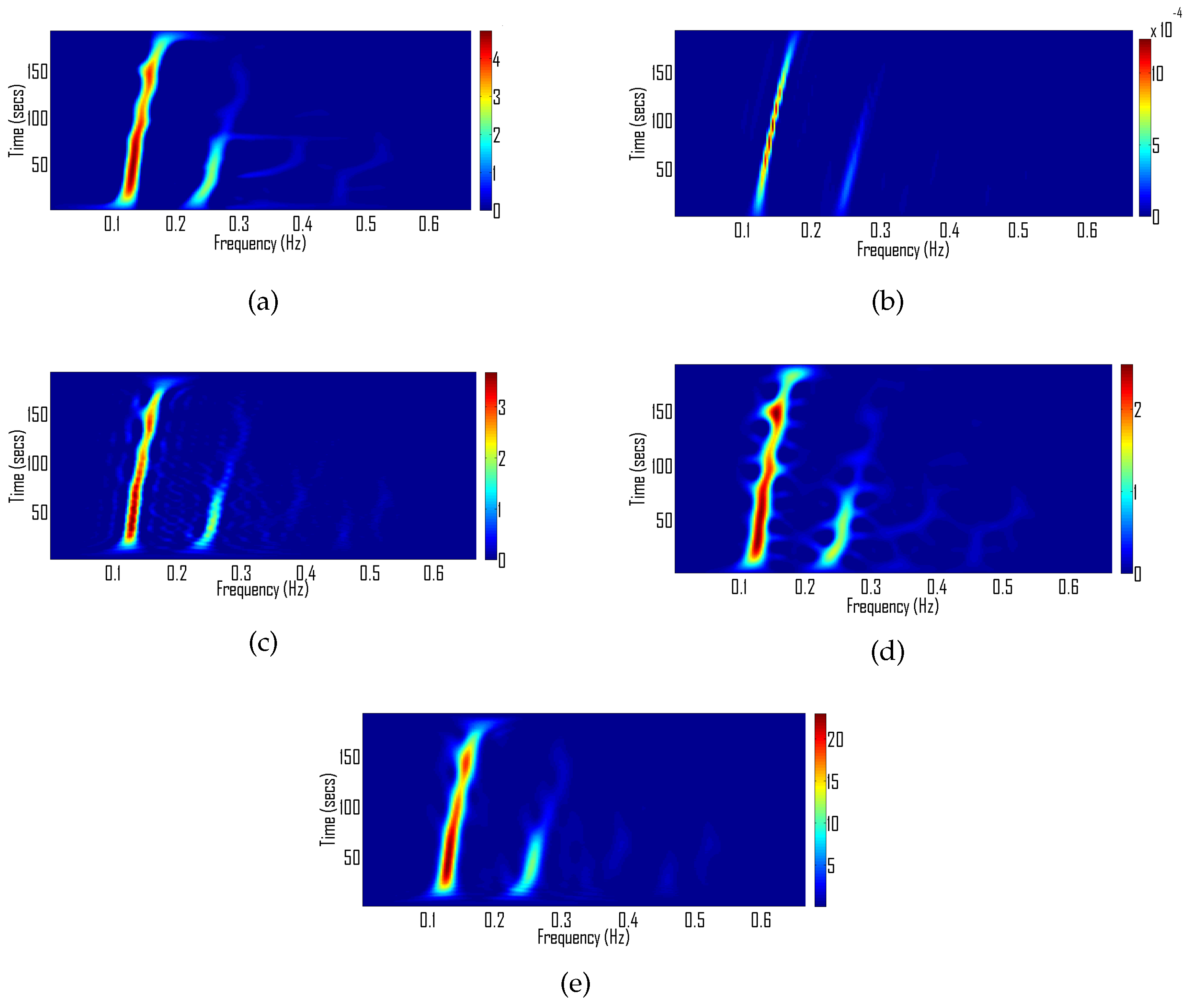
4.1. Performance Comparison Based on Energy Concentration

4.1.1. Measured Signals

The measured HR signals are down-sampled to 1.33 Hz and analysed using quadratic TFDs including the described methods, ADTFD, AOKTFD, MBD, S-method and the spectrogram where $N=424$ and $M=512$. Figure 2 illustrates that the ADTFD results in high energy concentration of both weak and strong signal components while no other TF method was able to achieve high energy concentration for the weak component. The aforementioned experiment is then repeated on 35 such HRV signals, and, for each TFD, the energy concentration measure in Equation (25) is computed. The mean and standard deviation of the energy concentration measure for all the TFDs are shown in

Table 1. Performance comparison of time-frequency distributions (TFDs) for the analysis of measured heart rate variability (HRV) signal using the energy concentration measure.

TFD	ADTFD	AOKTFD	MBD	S-method	Spectrogram
EC (mean)	0.8554 $\times {10}^4$	1.4576 $\times {10}^4$	1.4129 $\times {10}^4$	1.4298 $\times {10}^4$	1.6417 $\times {10}^4$
EC (standard deviation)	1.5582 $\times {10}^3$	3.3485 $\times {10}^3$	2.2148 $\times {10}^3$	2.2651 $\times {10}^4$	2.9416 $\times {10}^3$

The time-frequency distributions (TFDs) used are adaptive directional time-frequency distribution (ADTFD), adaptive optimal kernel time-frequency distribution (AOKTFD), modified B distribution (MBD), S-method and Spectrogram.

. The ADTFD achieves the minimum value and then also the highest energy concentration. In order to examine if the results are statistically significant between the ADTFD and the other TFDs described in Section 3, we perform a student’s t-test. In all cases, the p-values are less than $0.0001$.

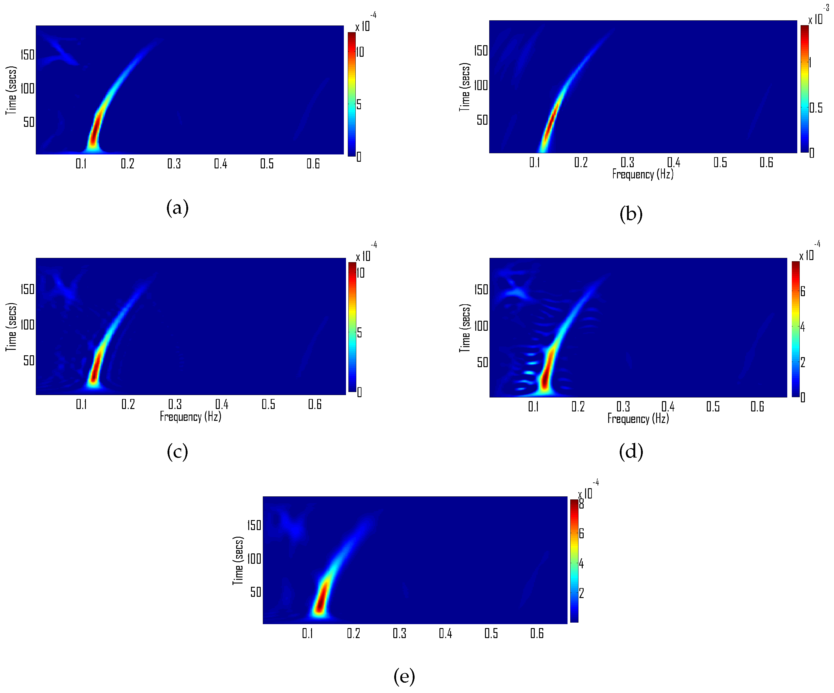
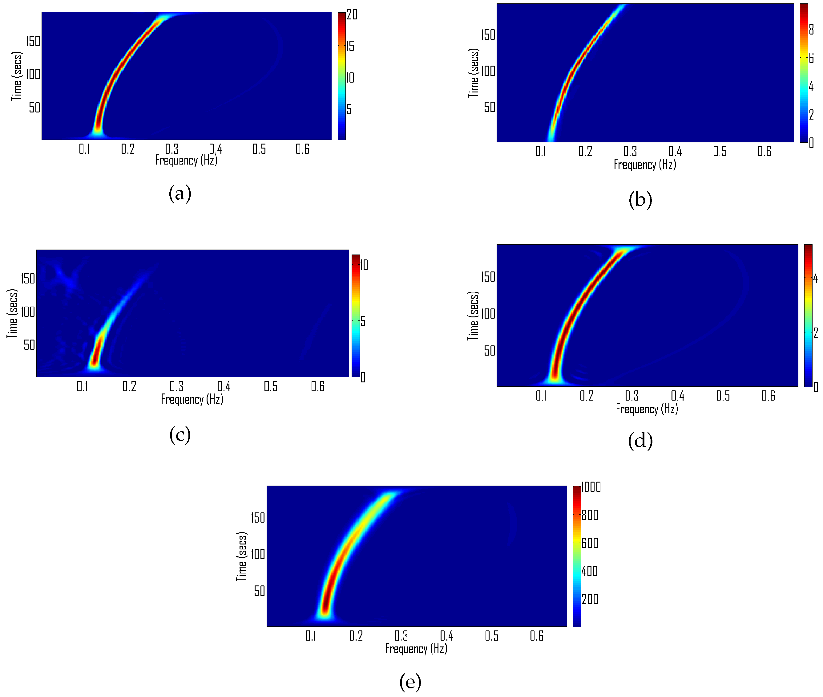
4.1.2. Simulated Signals

The experiment is repeated for synthetic signals using the IPFM and the AM–FM model described in Section 3. The synthetic signals are sampled at 1.33 Hz and analyzed using the same set of TFDs that were used for the measured signals.

The TF representations obtained using the IPFM and the AM–FM model are shown in Figure 3 and Figure 4, respectively. In both cases, the ADTFD achieves the highest energy concentration of auto-terms for both strong and weak signal components, while significantly reducing cross-terms. The energy concentration measures for the IPFM and the AM–FM model are shown in

Table 2. Performance comparison of TFDs for the analysis of simulated HRV signal based on the integral pulse frequency model.

TFD	ADTFD	AOKTFD	MBD	S-method	Spectrogram
EC	7.0524 $\times {10}^3$	1.5547 $\times {10}^4$	1.5241 $\times {10}^4$	1.4872 $\times {10}^4$	1.8622 $\times {10}^4$

and

Table 3. Performance comparison of TFDs for the analysis of simulated HRV signal based on the Amplitude Modulation-Frequency Modulation model.

TFD	ADTFD	AOKTFD	MBD	S-method	Spectrogram
EC	3.7660 $\times {10}^3$	9.2798 $\times {10}^3$	1.0854 $\times {10}^4$	6.6109 $\times {10}^3$	1.0974 $\times {10}^4$

, respectively. The ADTFD achieves the lowest value, implying the highest concentration and thus confirming the results of the visual assessment.

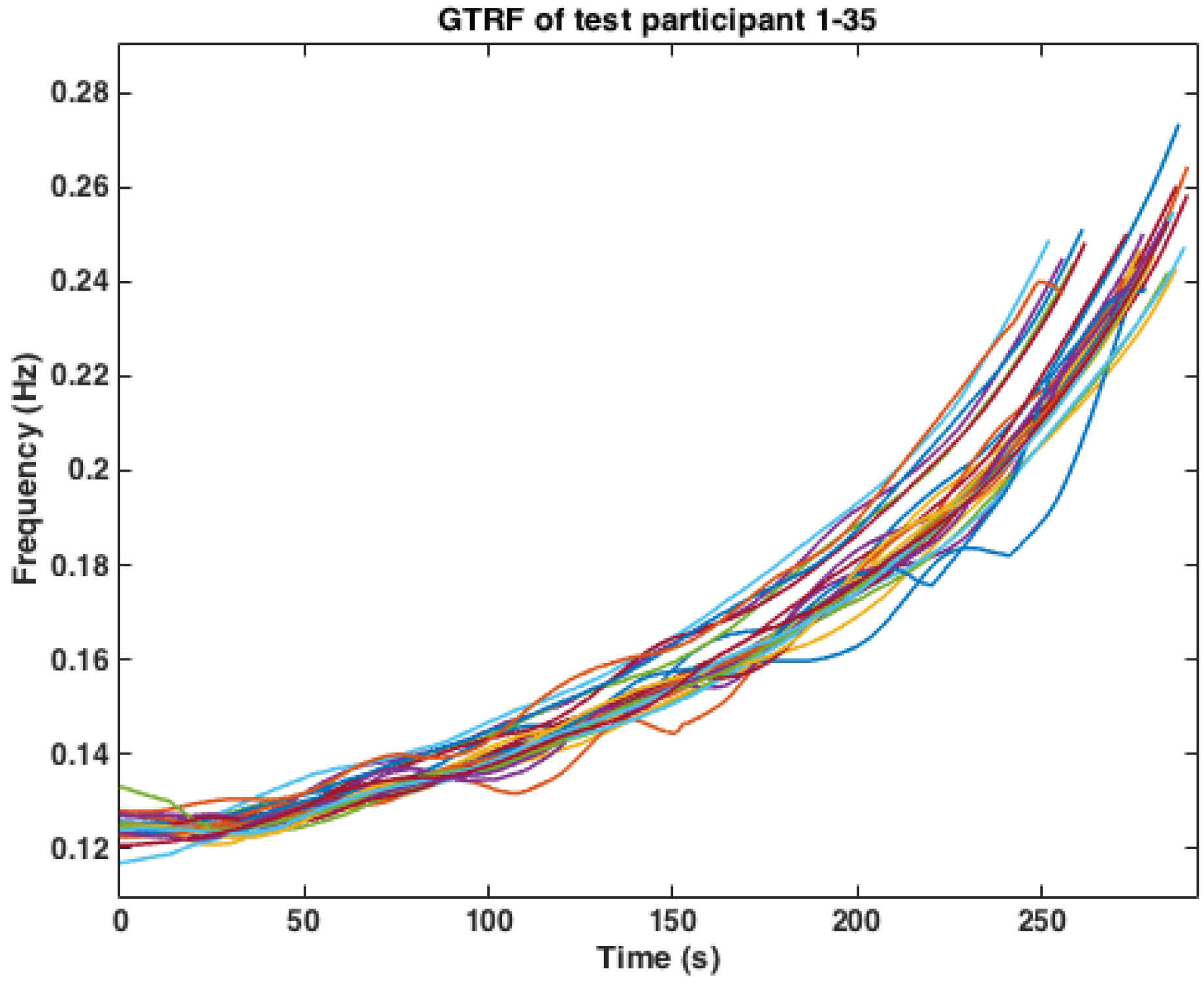
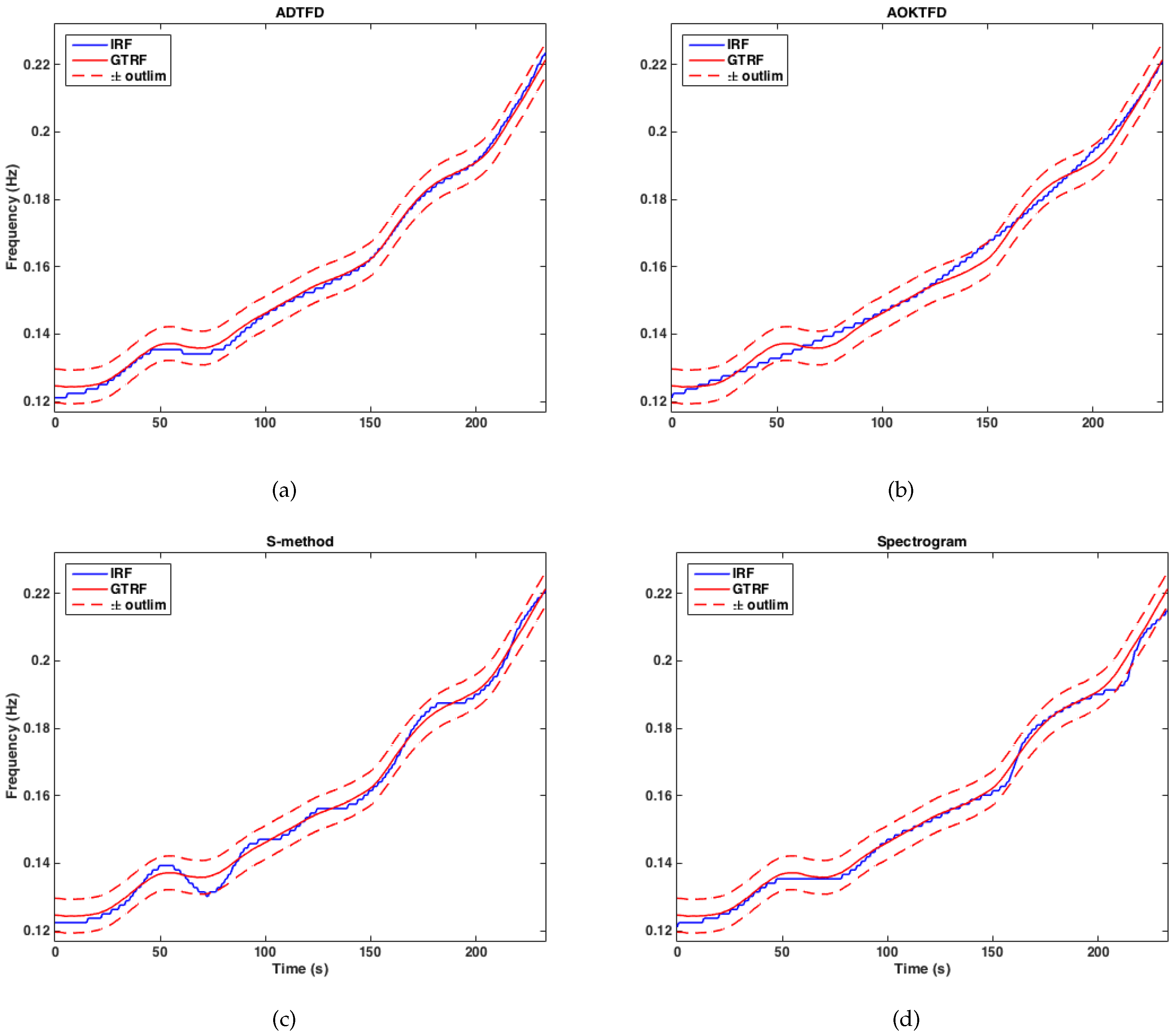
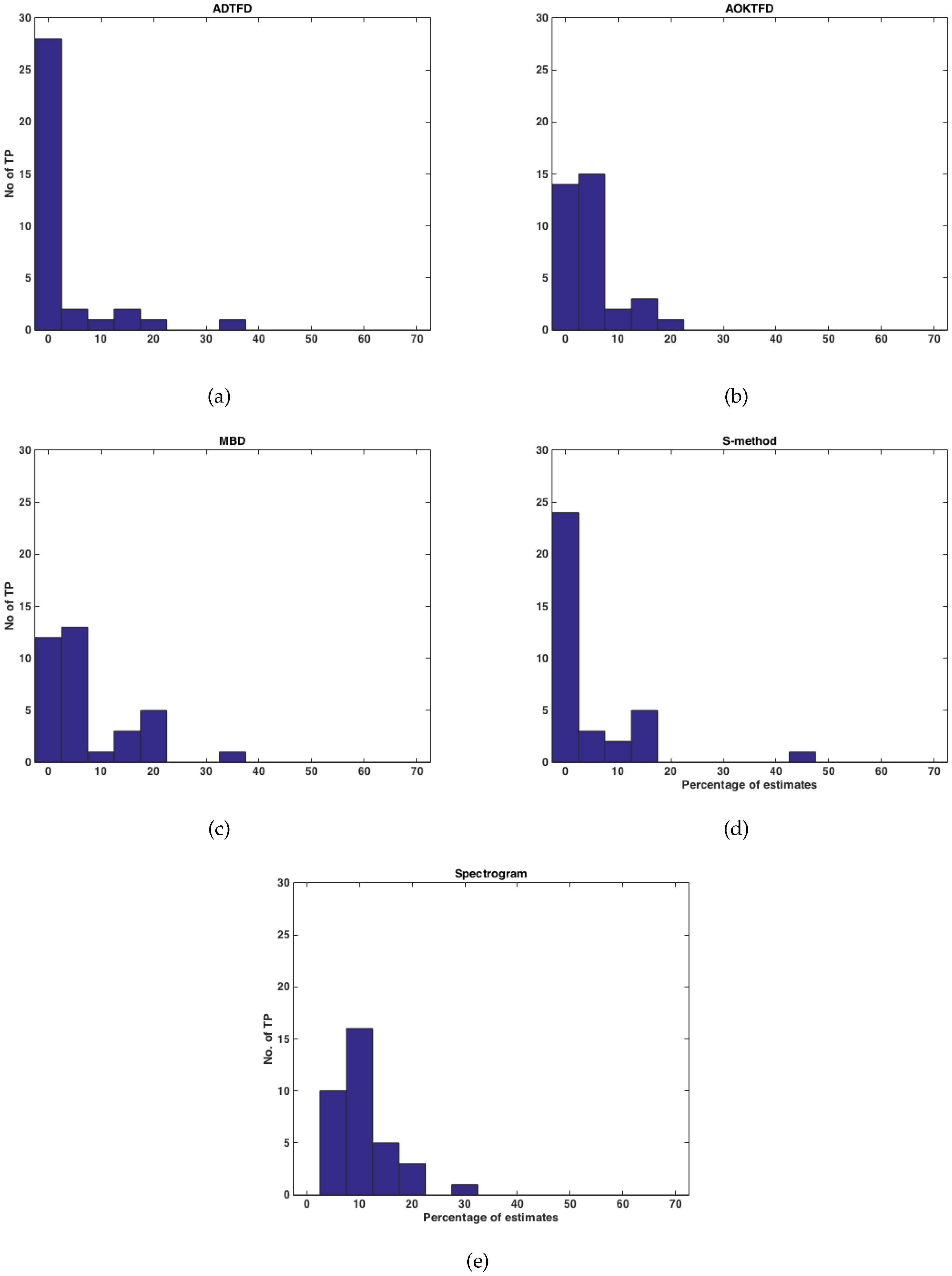
4.2. Accuracy of the Instantaneous Respiratory Frequency Estimate

From the HRV TF-images, the instantaneous respiratory frequency (IRF) is estimated as the maximum value at each time instant. Figure 5 illustrates the IF estimates (red solid lines) obtained using the ADTFD, AOKTFD, the S-method and the spectrogram together with the GTRF (blue solid lines). Note that the MBD method is omitted as the appearance of the estimate was similar to the AOKTFD. Differences between methods can be seen, where the ADTFD is more precise in the estimation of the faster variations in the respiratory frequency than other methods, e.g., the AOKTFD, which seems to over-estimate the oscillations, see Figure 5c) between frequencies 0.12–0.14 Hz. The experiment is repeated for all TPs. The grand average MSE is calculated and presented in

Table 4. Grand average mean square error of all test participants and all instantaneous respiratory frequency estimates.

TFD	ADTFD	AOKTFD	MBD	S-method	Spectrogram
gr.av.MSE	0.0656 $\times {10}^{-3}$	0.0387 $\times {10}^{-3}$	0.111 $\times {10}^{-3}$	0.0633 $\times {10}^{-3}$	0.0668 $\times {10}^{-3}$

for all methods. The smallest value is given from AOKTFD followed by the S-method, ADTFD and the spectrogram. However, the MSE is too sensitive to large deviations at few time points (outliers). Thus, few outliers can degrade the MSE performance for a method which is otherwise consistent in giving good results. In HRV spectra, a narrow band around the IF is important for estimating RSA related signal energy. Thus, a more reliable method for estimating the IF is one that generates a minimum number of outliers outside this band. In order to test the consistency of selected TFDs, we choose to apply an outlier limit (outlim) that is set to be 0.005 Hz.

The results of all 35 TPs indicate that the ADTFD is the most reliable method to estimate the IRF. The ADTFD based method was able to accurately estimate all frequency values inside the outlier (between the dashed red lines) in 25 out of total of 35 TPs (71.4%). The results of the other methods are not in this range (see

Table 5. Number and percentage of the TPs without any outlier IRFs.

TFD	ADTFD	AOKTFD	MBD	S-method	Spectrogram
No. of TPs (perc.)	25 (71.4%)	10 (28.6%)	5 (14.3%)	15 (42.9%)	0 (0%)

) and, especially, the spectrogram gives unreliable results, as none of the subjects has all estimates inside the outlier limits.

In Figure 6, histograms of the number of TPs that have a certain percentage of the IRFs outside the outlier limits are presented for all methods. The ADTFD results in nine TPs where less than 20% of the IRFs are outliers, and only one TP with higher rate. For the AOKTFD, 25 TPs have up to 20% outlier values, a significant error that is in most cases caused by the AOKTFD method disability to follow fast frequency changes. The MBD method has a similar behavior and the S-method gives a number of 19 TPs with outlier rates up to 15%, where the spectrogram gives at least up to 20% outliers for almost all subjects included in the study.

5. Conclusions

A comparison of the state of art TF distributions has been performed for the estimation of instantaneous respiratory frequency (IRF) from the heart rate variability signal. The ability of time-frequency distributions (TFD) to concentrate signal energy in the time-frequency domain and accurately estimate the peak heart rate variability frequency was used as performance criteria. For estimating energy concentration of a TFD, we used the measure developed in [45]. For estimating the accuracy of the IRF estimate, the instantaneous frequency estimate from the respiratory signal was used as a reference signal. It was noted that the adaptive directional time-frequency distribution (ADTFD), due to its local time-frequency kernel, was able to achieve high energy concentration for both weak and strong components. The ADTFD also has superior performance to avoid outlier estimates as well as to accurately follow frequency changes. As a result, the ADTFD based method gave the most reliable estimate of IRF in 25 out of total of 35 test participants. The next best performance was achieved by the S-method that correctly estimated IRFs for only 15 test participants.

The present study indicates that the IRF can be reliably estimated from ECG recordings without requiring additional acquisition of the respiratory frequency. An accurate estimation of the IRF is crucial for a more reliable estimate of HF-HRV based on the more narrow frequency band around the IRF. The narrow band HF-HRV can be shown to give more reliable measures of clinical importance such as diagnosis of coronary artery diseases and other cardiac disorders. In future research, we will apply time-frequency filtering algorithms with the aim to improve estimates of the narrow band HF-HRV power using the IRF estimated from the respiratory related frequency of the HRV signal.

References

1. Task Force of the European Society of Cardiology and the North American Society of Pacing and Electrophysiology. Heart rate variability: Standards of measurement, physiological interpretation, and clinical use. Eur. Heart J. 1996, 17, 354–381. [Google Scholar]
2. Porges, S.W. Orienting in a defensive world: Mammalian modification of our evolutionary heritage. A polyvagal theory. Psychophysiology 1995, 32, 301–318. [Google Scholar] [CrossRef] [PubMed]
3. Porges, S.W. The polyvagal perspective. Biol. Psychol. 2007, 74, 116–143. [Google Scholar] [CrossRef] [PubMed]
4. Gates, K.M.; Gatzke-Kopp, L.M.; Sandsten, M.; Blandon, A.Y. Estimating time-varying RSA to examine psychophysiological linkage of marital dyads. Psychophysiology 2015. [Google Scholar] [CrossRef] [PubMed]
5. Dolatabadi, A.D.; Khadem, S.E.Z.; Asl, B.M. Automated diagnosis of coronary artery disease (CAD) patients using optimized SVM. Comput. Methods Progr. Biomed. 2017, 138, 117–126. [Google Scholar] [CrossRef] [PubMed]
6. Levine, J.; Fleming, R.; Piedmont, J.I.; Cain, S.M.; Chen, W.J. Heart rate variability and generalized anxiety disorder during laboratory-induced worry and aversive imagery. J. Affect. Disord. 2016, 205, 207–215. [Google Scholar] [CrossRef] [PubMed]
7. Thayer, J.F.; Yamamoto, S.S.; Brosschot, J.F. Review: The relationship of autonomic imbalance, heart rate variability and cardiovascular disease risk factors. Int. J. Cardiol. 2010, 141, 122–131. [Google Scholar] [CrossRef] [PubMed]
8. Hansson, M.; Jönsson, P. Estimation of HRV spectrogram using multiple window methods focussing on the high frequency power. Med. Eng. Phys. 2006, 28, 749–761. [Google Scholar] [CrossRef] [PubMed]
9. Hansson-Sandsten, M.; Jönsson, P. Multiple window correlation analysis of HRV power and respiratory frequency. IEEE Trans. Biomed. Eng. 2007, 54, 1770–1779. [Google Scholar] [CrossRef] [PubMed]
10. Melkonian, D.; Korner, A.; Meares, R.; Bahramali, H. Increasing sensitivity in the measurement of heart rate variability: The method of non-stationary RR time-frequency analysis. Comput. Methods Progr. Biomed. 2012, 108, 53–67. [Google Scholar] [CrossRef] [PubMed]
11. Bailón, R.; Sörnmo, L.; Laguna, P. A robust method for ECG-based estimation of the respiratory frequency during stress testing. IEEE Trans. Biomed. Eng. 2006, 53, 1273–1285. [Google Scholar] [CrossRef] [PubMed]
12. Bailón, R.; Mainardi, L.; Orini, M.; Sörnmo, L.; Laguna, P. Analysis of heart rate variability during exercise stress testing using respiratory information. Biomed. Signal Proc. Control 2010, 5, 299–310. [Google Scholar] [CrossRef]
13. Hernando, A.; Lazaro, J.; Gil, E.; Arza, A.; Garzon, J.M.; Lopez-Anton, R.; de la Camara, C.; Laguna, P.; Aguilo, J.; Bailon, R. Inclusion of respiratory frequency information in heart rate variability analysis for stress assessment. IEEE J. Biomed. Health Inform. 2016, 20, 1016–1025. [Google Scholar] [CrossRef] [PubMed]
14. Stark, R.; Schienle, A.; Walter, B.; Vaitl, D. Effects of paced respiration on heart period and heart period variability. Psychophysiology 2000, 37, 302–309. [Google Scholar] [CrossRef] [PubMed]
15. Song, H.; Lehrer, P.M. The effects of specific respiratory rates on heart rate and heart rate variability. Appl. Psychophysiol. Biofeedback 2003, 28, 13–23. [Google Scholar] [CrossRef] [PubMed]
16. Grossman, P.; Taylor, E.W. Toward understanding respiratory sinus arrhythmia: Relations to cardiac vagal tone, evolution and biobehavioral functions. Biol. Psychol. 2007, 74, 263–285. [Google Scholar] [CrossRef] [PubMed]
17. Schäfer, A.; Kratky, K.W. Estimation of breathing rate from respiratory sinus arrhythmia: Comparison of Various Methods. Ann. Biomed. Eng. 2008, 36, 476–485. [Google Scholar] [CrossRef] [PubMed]
18. Ebrahimi, F.; Setarehdan, S.K.; Nazeran, H. Automatic sleep staging by simultaneous analysis of ECG and respiratory signals in long epochs. Biomed. Signal Proc. Control 2015, 18, 69–79. [Google Scholar] [CrossRef]
19. Lenis, G.; Kircher, M.; Lázaro, J.; Bailón, R.; Gil, E. Separating the effect of respiration on the heart rate variability using Granger’s causality and linear filtering. Biomed. Signal Proc. Control 2017, 31, 272–287. [Google Scholar] [CrossRef]
20. Sekhar, S.C.; Sreenivas, T.V. Adaptive spectrogram vs. adaptive pseudo-Wigner-Ville distribution for instantaneous frequency estimation. Signal Proc. 2003, 83, 1529–1543. [Google Scholar] [CrossRef]
21. Malarvili, M.B.; Mesbah, M. Newborn seizure detection based on heart rate variability. IEEE Trans. Biomed. Eng. 2009, 56, 2594–2603. [Google Scholar] [CrossRef] [PubMed]
22. Hlawatsch, F.; Boudreaux-Bartels, G.F. Linear and quadratic time-frequency signal representations. IEEE Signal Proc. Mag. 1992, 9, 21–67. [Google Scholar] [CrossRef]
23. Auger, F.; Flandrin, P.; Lin, Y.T.; McLaughlin, S.; Meignen, S.; Oberlin, T.; Wu, H.T. Time-frequency reassignment and synchrosqueezing: An overview. IEEE Signal Proc. Mag. 2013, 30, 32–41. [Google Scholar] [CrossRef] [Green Version]
24. Lin, Y.T.; Wu, H.T. ConceFT for time-varying heart rate variability analysis as a measure of noxious stimulation during general anesthesia. IEEE Trans. Biomed. Eng. 2017, 64, 145–154. [Google Scholar] [CrossRef] [PubMed]
25. Wu, H.T.; Wu, H.K.; Wang, C.L.; Yang, Y.L.; Wu, W.H.; Tsai, T.H.; Chang, H.H. Modeling the pulse signal by wave-shape function and analyzing by synchrosqueezing transform. PLoS ONE 2016, 11, e0157135. [Google Scholar] [CrossRef] [PubMed]
26. Boashash, B.; Khan, N.A.; Ben-Jabeur, T. Time–frequency features for pattern recognition using high-resolution TFDs: A tutorial review. Digit. Signal Proc. 2015, 40, 1–30. [Google Scholar] [CrossRef]
27. Barkat, B.; Boashash, B. A high-resolution quadratic time-frequency distribution for multicomponent signals analysis. IEEE Trans. Signal Proc. 2001, 49, 2232–2239. [Google Scholar] [CrossRef]
28. Stevenson, N.; Mesbah, M.; Boashash, B. Quadratic time-frequency distribution selection for seizure detection in the newborn. In Proceedings of the 30th Annual International Conference of the IEEE Engineering in Medicine and Biology Society, Vancouver, BC, Canada, 20–25 August 2008; pp. 923–926.
29. Stanković, L.J. A method for time-frequency analysis. IEEE Trans. Signal Proc. 1994, 42, 225–229. [Google Scholar] [CrossRef]
30. Orović, I.; Stanković, S. Time-frequency-based speech regions characterization and eigenvalue decomposition applied to speech watermarking. EURASIP J. Adv. Signal Proc. 2010, 2010, 572748. [Google Scholar] [CrossRef]
31. Stanković, L.; Thayaparan, T.; Daković, M.; Popović, V. S-method in radar imaging. In Proceedings of the 14th European Signal Processing Conference, Florence, Italy, 4–8 September 2006; pp. 1–5.
32. Jones, D.L.; Baraniuk, R.G. An adaptive optimal-kernel time-frequency representation. IEEE Trans. Signal Proc. 1995, 43, 2361–2371. [Google Scholar] [CrossRef]
33. Khan, N.A.; Boashash, B. Multi-component instantaneous frequency estimation using locally adaptive directional time frequency distributions. Int. J. Adapt. Control Signal Proc. 2016, 30, 429–442. [Google Scholar] [CrossRef]
34. Khan, N.A.; Ali, S. Classification of EEG signals using adaptive time-frequency distributions. Metrol. Meas. Syst. 2016, 23, 251–260. [Google Scholar] [CrossRef]
35. Khan, N.A.; Ali, S.; Jansson, M. Direction of arrival estimation using adaptive directional time-frequency distributions. Multidimens. Syst. Signal Proc. 2016, 1–19. [Google Scholar] [CrossRef]
36. Stanković, L.; Djurović, I.; Stanković, S.; Simeunović, M.; Djukanović, S.; Daković, M. Instantaneous frequency in time–frequency analysis: Enhanced concepts and performance of estimation algorithms. Digit. Signal Proc. 2014, 35, 1–13. [Google Scholar] [CrossRef]
37. Huang, N.E.; Shen, Z.; Long, S.R.; Wu, M.C.; Shih, H.H.; Zheng, Q.; Yen, N.C.; Tung, C.C.; Liu, H.H. The empirical mode decomposition and the Hilbert spectrum for nonlinear and non-stationary time series analysis. Proc. R. Soc. Lond. A Math. Phys. Eng. Sci. 1998, 454, 903–995. [Google Scholar] [CrossRef]
38. Altan, G.; Kutlu, Y.; Allahverdi, N. A new approach to early diagnosis of congestive heart failure disease by using Hilbert-Huang transform. Comput. Methods Progr. Biomed. 2016, 137, 23–34. [Google Scholar] [CrossRef] [PubMed]
39. Xie, H.; Wang, Z. Mean frequency derived via Hilbert-Huang transform with application to fatigue EMG signal analysis. Comput. Methods Progr. Biomed. 2006, 82, 114–120. [Google Scholar] [CrossRef] [PubMed]
40. Oweis, R.J.; Abdulhay, E.W. Seizure classification in EEG signals utilizing Hilbert-Huang transform. Biomed. Eng. Online 2011, 10, 38. [Google Scholar] [CrossRef] [PubMed]
41. Khan, N.A.; Boashash, B. Instantaneous frequency estimation of multicomponent nonstationary signals using multiview time-frequency distributions based on the adaptive fractional spectrogram. IEEE Signal Proc. Lett. 2013, 20, 157–160. [Google Scholar] [CrossRef]
42. Cohen, L. Time-frequency distributions—A review. Proc. IEEE 1989, 77, 941–981. [Google Scholar] [CrossRef]
43. Hlawatsch, F. Interference terms in the Wigner distribution. Digit. Signal Proc. 1984, 84, 363–367. [Google Scholar]
44. Sejdić, E.; Djurović, I.; Jiang, J. Time–frequency feature representation using energy concentration: An overview of recent advances. Digit. Signal Proc. 2009, 19, 153–183. [Google Scholar] [CrossRef]
45. Stanković, L. A measure of some time–frequency distributions concentration. Signal Proc. 2001, 81, 621–631. [Google Scholar] [CrossRef]
46. MacFarland, T.W. Student’s t-Test for Independent Samples. In Introduction to Data Analysis and Graphical Presentation in Biostatistics with R: Statistics in the Large; Springer: Cham, Switzerland, 2014; pp. 17–46. [Google Scholar]
47. Bailón, R.; Laouini, G.; Grao, C.; Orini, M.; Laguna, P.; Meste, O. The integral pulse frequency modulation model with time-varying threshold: Application to heart rate variability analysis during exercise stress testing. IEEE Trans. Biomed. Eng. 2011, 58, 642–652. [Google Scholar] [CrossRef] [PubMed]
48. Boashash, B. Advances in Spectral Analysis and Array Processing; Prentice Hall: Englewood Cliff, NJ, USA, 1991; pp. 418–517. [Google Scholar]
Figure 1. The ground truth respiratory frequencies (GTRF), estimated from the spectrogram maximum peak values of the corresponding respiratory frequencies of test participants (TP) 1-35.
Applsci 07 00221 g001
Figure 2. Time-frequency (TF) analysis of measured heart rate signals; (a) adaptive directional time-frequency distribution (ADTFD) ( a = 3 , b = 8 ); (b) Adaptive Optimal Kernel Time-frequency Distribution (AOKTFD); (c) modified B distribution (MBD) ( β = 0 . 05 , lag window = 64); (d) S-method (Short time Fourier transform (STFT) window length = 91, frequency axis convolution window length = 21); (e) Spectrogram (window length = 91).
Applsci 07 00221 g002
Figure 3. TF analysis of simulated HR signals based on the integral pulse frequency model (IPFM); (a) ADTFD ( a = 3 , b = 8 ); (b) AOKTFD; (c) MBD ( η = 0 . 05 , lag window = 64); (d) S-method (STFT window length = 91, frequency axis convolution window length = 21); (e) spectrogram (window length = 91).
Applsci 07 00221 g003
Figure 4. TF analysis of simulated HR signals based on the Amplitude Modulation-Frequency Modulation (AM-FM) model; (a) ADTFD ( a = 3 , b = 8 ); (b) AOKTFD; (c) MBD ( η = 0 . 05 , lag window = 64); (d) S-method (STFT window length = 91, frequency axis convolution window length = 21); (e) Spectrogram (window length = 91).
Applsci 07 00221 g004
Figure 5. The estimated HRV peak frequency from TP 11 and the corresponding ground truth respiratory frequency (GTRF). The dashed lines represents the outlier limit (outlim = 0.005 Hz); (a) ADTFD ( a = 3 , b = 8 ); (b) AOKTFD; (c) S-method (STFT window length = 91, frequency axis convolution window length = 21); (d) spectrogram (window length = 91).
Applsci 07 00221 g005
Figure 6. The number of TPs (out of the total of 35 patients) corresponding to a certain percentage of estimated IRF values found outside the outlier limits; (a) ADTFD ( a = 3 , b = 8 ); (b) AOKTFD; (c) MBD ( η = 0 . 05 , lag window = 64); (d) S-method (window length for short time-Fourier is 91 and window length for performing convolution along frequency axis is 21); (e) spectrogram (window length 91).
Applsci 07 00221 g006