
ANN Sizing Procedure for the Day-Ahead Output Power Forecast of a PV Plant


Department of Energy, Politecnico di Milano, 20156 Milano, Italy
*
Author to whom correspondence should be addressed.
Appl. Sci. 2017, 7(6), 622; https://0-doi-org.brum.beds.ac.uk/10.3390/app7060622
Submission received: 4 May 2017
/
Revised: 5 June 2017
/
Accepted: 12 June 2017
/
Published: 15 June 2017
(This article belongs to the Special Issue Computational Intelligence in Photovoltaic Systems)
Abstract
:Since the beginning of this century, the share of renewables in Europe’s total power capacity has almost doubled, becoming the largest source of its electricity production. In 2015 alone, photovoltaic (PV) energy generation rose with a rate of more than 5%; nowadays, Germany, Italy, and Spain account together for almost 70% of total European PV generation. In this context, the so-called day-ahead electricity market represents a key trading platform, where prices and exchanged hourly quantities of energy are defined 24 h in advance. Thus, PV power forecasting in an open energy market can greatly benefit from machine learning techniques. In this study, the authors propose a general procedure to set up the main parameters of hybrid artificial neural networks (ANNs) in terms of the number of neurons, layout, and multiple trials. Numerical simulations on real PV plant data are performed, to assess the effectiveness of the proposed methodology on the basis of statistical indexes, and to optimize the forecasting network performance.
1. Introduction
The recent increase of renewable energy sources (RES) quota in power systems is facing new technical challenges, involving also the overall efficiency of the electrical grid [1]. Therefore, several techniques able to forecast the output power of RES facilities have been developed, in particular addressing the inherent variability of parameters related to solar radiation and atmospheric weather, which directly affect photovoltaic (PV) systems’ power output [2]. Robust predictive tools based on the measured historical data of a specific PV plant can provide advantages in its operation policy, in order to avoid or minimize excess production, and to benefit from the available incentives for producing electricity from RES [3]. Moreover, the increasing penetration of accurate forecasting models, constrained by the market and incentives, can implicitly facilitate the alignment of producers’ decisions with energy policy and emissions targets.
In particular, these predictive models are aimed at finding out the relationship between the numerical weather prediction and the forecasted power output [4]. However, any forecasting activity of natural phenomena is characterized by a high degree of non-linearity. To address this complexity, artificial neural networks (ANNs) with a multilayer perceptron (MLP) architecture are often used. These are a class of machine learning (ML) techniques used to solve specific kinds of problems, such as: pattern recognition, function approximation, control, and forecasting [5,6,7].
ANNs are known as a very flexible tool, and several layouts have been developed to solve different tasks [8]. In particular, ML forecasting methods can be used on an extended dataset of historical measurements, providing an advantage in reducing prediction errors with respect to other statistical and physical forecasting models [9,10]. An additional advantage of ML techniques is their ability to handle missing data and to solve problems with a high degree of complexity.
The first breakthroughs in using ML technologies in the solar power forecasting field were pioneered more than a decade ago [11]. A comprehensive review of solar power forecast approaches is given in [12]; this paper provides a systematic discussion comparing and contrasting many works on applying artificial neural networks to the PV forecasting problem. ML techniques are demonstrated to be successfully applied for this purpose, provided that suitable historical patterns are available. In addition, the potential benefits of hybrid techniques, such as those in [13,14], are also thoroughly discussed.
Nowadays, in the case of a particular PV plant’s power output, the common training data are the historical measurements of power production, and the meteorological parameters related to the specific plant’s location, which include temperature, global horizontal irradiance, and cloud cover above the facility. Additional forecasted variables from numerical weather predictions can also be considered, such as wind speed, humidity, and pressure.
Recently, novel forecasting models have been implemented by adding an estimate of the clear sky radiation to the series of historical local weather data, in order to hybridize the meteorological forecasts with physical data, as reported in [15].
Moreover, the effectiveness of using ensemble methods, i.e., running simultaneously a number of parallel neural networks and finally averaging their results, was demonstrated in [16], thus giving additional advantages also to modern parallel computing techniques. The same paper also shows the response of the network to changes in training set size and meteorological conditions.
In this paper, the authors present a procedure to set up the main characteristics of the network using a physical hybrid method (PHANN) to perform the day-ahead PV power forecast in view of the electricity market. The procedure outlined here can be adopted to set up the best settings of the network in terms of the number of layers, neurons, and trials. Once all the optimum settings have been identified after this procedure, it is possible to perform the day-ahead forecast with the PHANN method using different sets for training and validation. The test data set will be made up of the 24 hourly PV power values forecasted one day ahead.
The paper is structured as follows: Section 2 provides an overview of the considered neural network architectures. Section 3 presents the methodology implemented to compare different ANN structures and dimensions, and Section 4 will propose some metrics aimed at evaluating each configuration’s suitability in terms of error performance and statistical behavior. Section 5 presents the considered case study, which is used to test the proposed methodology in terms of the number of layers, neurons and the size of the ensemble. Specific simulations and numerical results are provided in Section 6, Section 7 and Section 8, and final remarks are reported in Section 9.
2. Artificial Neural Networks
An ANN basically consists of a number of neurons, grouped in different layers, which receive input from all of the neurons in the preceding layer. Each neuron performs a simple nonlinear operation, and the learning capacity is finite due to the number of neurons and links existing among them. The number of neurons in the first input layer is equal to the number of input data, and the number of neurons in the output layer corresponds to the number of output values. Hidden layers are in between, and their neurons can vary in number.
Choosing the amount of neurons in the layers and the number of layers depends on several factors, as well as the kind problem to be addressed [17]. There are several proposed models to define an optimal network [18], but these methods are not applicable to every area of study. Indeed, the success of a network depends heavily on the experience of the creator [19], and many attempts must be made to reach satisfactory result. Moreover, some limits are imposed by the computational burden. In fact, the more complex the network, the longer the time (hours) needed for data processing.
This paper describes a heuristic process, by means of a statistical indicators comparison, in order to optimize the settings of a Feed Forward Neural Network (FFNN) for PV forecasting based on weather predictions. The search for the best layout is constrained by computational limitations. For the above mentioned FFNN, the most effective configuration based on the minimum absolute mean error (normalized or weighted) index has been studied. Since the future weather conditions are unknown at the time of prediction, it is impossible to determine a priori which precise network layout will provide the best PV power production forecast.
It must be pointed out that, during the FFNN training step, both the input (i.e., the historical weather forecasts) and the target (i.e., the historical PV plant output power) datasets employed are just one representative couple of the virtually infinite couples of input and target presented in the historical weather data pool.
Furthermore, for any given dataset, each network configuration presents an additional element of randomness. In fact, for a specific network layout, the training process is initialized by means of randomly chosen weights and biases; therefore, for the same forecast, the performance is non-unique.
Hence, to set up the main settings, it is useful to feed the FFNN with the same data that is representative of the majority of the possible mutations incurring in the dataset. A one-year dataset represents a valid data sample, as it spans over periods of different weather conditions. Still, if the network deals with a climatically unusual day forecast, a worsening of the performance should be expected.
3. Methodology
3.1. Early Assumptions
As one of the goals of this work is to study how the number of neurons in the ANN’s layers affects the forecast, and to consequently determine the optimal setup (that is, the solution that minimizes the errors), we will modify only the network settings, while keeping the same database. Since this is a stochastic method applied on the available dataset, an average performance must be evaluated, and often the “best solution” will not be unique.
In fact, two networks will provide different outputs even if equally configured to follow the same training process. This is due to the random initialization of weights and biases, which is peculiar for each training run. Therefore, comparing two networks with different settings only by looking at their output cannot generally lead to comprehensive answers. A rigorous approach towards stochastic elements is specifically needed, especially in the comparison between various network layouts and settings, when searching for the best possible configuration. Hence, FFNN has been analyzed by studying the output of the network as a function of the number of neurons and their layout. In each study, the neuron activation function was kept unchanged, and we used the tan-sigmoid (“tansig” in Matlab Neural Network Toolbox™, R2016a, MathWorks®, Natick, MA, USA [20]), which has the following expression, where x is the generic input and y the output of the neuron:
Here, two “similar networks” are defined as two networks with the same topology (number of neurons and their layout), but with different weights and biases. Therefore, statistic tools are used to infer more tangible conclusions, giving more strength to the final settings adopted by the method.
3.2. Data Set Definition
In order to perform the forecast, historical data are provided to the Neural Network Toolbox™ [20] in Matlab software, R2016a, MathWorks®, Natick, MA, USA, and grouped in three clusters: “training”, “validation”, and “test”. Each group fulfills three specific tasks:
- (1)
- The training set includes the samples employed to train the network. It should contain enough different examples (days) to make the network able to generalize its learning.
- (2)
- The validation set contains additional samples (i.e., days not already included in the training set) used by the network to check and validate the training process.
- (3)
- The test set is the dataset corresponding to the days actually forecasted by the network.
3.3. Artificial Neural Network Size
The ANN sizing problem primarily means to choose how many neurons are in the layers, and their layout. The neurons (or units) in the input and output layers are fixed by the problem to be solved, while characterizing the neurons in the hidden layers is controversial, since the hidden neurons are regarded as the processing neurons in the network. In addition, having a small number of hidden layers might increase the speed of the training process, whereas a large number of hidden layers could make it longer. Furthermore, the nonlinearity capability of an ANN increases with the number of layers; i.e., the more complicated (nonlinear) the input/output relationship is, the more layers an ANN will need to model it. In addition, the greater the number of neurons per layer, the more accurately can ANNs identify input/output relationships. In order to guarantee a sufficient generalization capability for the ANN, the number of neurons is reasonably bound to the training set size. Though, from the literature, only some general conditions and intuitive rules could be inferred.
In Widrow’s review [21], it is stated that the number of weights Nw existing within a layered ANN is bound to the number of patterns Np in the training set and outputs No by the following condition:
Condition (2) means that a given ANN should have an amount of neurons that is sufficiently smaller than the training samples. In fact, if the degrees of freedom (i.e., Nw) are larger than the constraints associated with the desired response function (i.e., No and Np), the training procedure will be unable to completely constrain the weights in the network.
In the mid-1960s, Cover studied the capacity of an FFNN with an arbitrary number of layers and a single output element [22,23]. In the same line, Baum and Haussler [21] addressed the question of the net size, which provides a valid generalization stating, with a desired accuracy of 90%, that at least 10 times as many training examples as there are weights in the ANN should be considered. In [24], the authors also provide theoretical lower and upper bounds on the sample size as a function of the net size, such that a valid generalization can be expected. However, they limited their study under the assumption that the node functions are linear threshold functions (or at least Boolean valued), leaving open the problem for classes of real valued functions (such as sigmoid functions), and multiple hidden layers networks.
To characterize the number of neurons in the layers, there are different rules suggested in the literature, starting from two incremental algorithms ([25] and the reference therein), passing through a trial and error procedure [26], to some thumb rules. For example, Chow et al. [27] applied—in the same forecasting context of this work—a thumb rule found in [28] in the “backpropagation architecture—standard connections” section. There, it is stated that the default number of hidden neurons Nn for a three layer network is computed with the following formula:
where i is the number of inputs; and o is the number of outputs. For more layers, it is stated that Nn should be divided by the number of hidden layers.
Finally, there is a symmetrical technique from the already mentioned tiling algorithm [29]. In the first, a small number of neurons is selected. Then, they are increased gradually. The symmetrical approach is referred to as the “pruning” algorithm [30]. This method, starting from a large network, carries on a gradual removal of the neurons by erasing the less significant units, and it requires in advance the largest size of the network [31].
Although the above cited approaches have a general value, in this paper the authors present a procedure to select the best settings of the neural network in terms of the number of layers, neurons, and trials, with the specific application of the physical hybrid method (PHANN) performing the day-ahead PV power forecast in view of the electricity market.
4. Evaluation Indexes
With respect to our specific application in PV power forecasting, although several evaluation indexes with different meanings are adopted in the literature, their trends are usually highly correlated, as they are calculated on the common basis of the hourly error :
which is the difference between the measured value of the output power Pm,h and the forecasted one Pp,h in the same hour h. Therefore, we now consider the normalized mean absolute error NMAE% as a reference for evaluating the performance of the forecasts:
The normalized mean absolute error NMAE% is based on the net capacity of the plant C. N is the number of time samples (hours) considered in the evaluated period (i.e., in a daily error basis calculation).
This index was calculated for the output “test set” of each individual network’s performance. As the NMAE% value is a random variable, its trend could be analyzed by means of the theory of parametric estimation. Therefore, when looking for the settings which on average minimize NMAE% values, the FFNN will be analyzed as a function of:
- (1)
- a single layer number of neurons;
- (2)
- a double layer number of neurons; and
- (3)
- trials in the ensemble forecast.
To proceed with this analysis, these steps are followed:
- (1)
- one or more ANN parameters are kept constant;
- (2)
- the free parameter to be inspected (i.e., number of neurons within a layer) is varied within a specific range; and
- (3)
- the NMAE% values of similar networks are calculated.
Under appropriate conditions, a range of values of the NMAE% can be calculated, assuming that the unknown mean of all of the possible NMAE% values, with those ANN settings, is within that interval of confidence.
NMAE Statistical Distributions and Confidence Limits
In order to study NMAE% behavior with respect to a specific ANN setting, this setting is assigned a starting constant value, and nt forecasts are performed. For each i-th forecast (trial), the NMAE% is calculated. From a statistical point of view, the group of these NMAE% values represents a sample of the endless population of all of the possible NMAE% values related to the forecast performed with those specific ANN settings. After the same parameter has been changed, further nt forecasts are performed, and the associated NMAE% values are calculated. This procedure is repeated until the maximum value of the ANN parameter is reached. As this value could be as great as possible, a reasonable threshold is set. Intuitively, a higher accuracy could be obtained by increasing the number of forecasts for each network, but the highly time-consuming process should be compensated for by a much more striking performance, otherwise it is not worthy. Therefore, a tradeoff between the computational burden and the expected accuracy is defined. Considering the group of NMAE% values belonging to the same test set obtained by the ANN with those given “p” settings, the relative sample mean is an estimator of all of the possible NMAE% values, and it is defined as:
where NMAEi,p is the NMAE% calculated for the i-th trial performed by the ANN with the p-th value of a given setting. In our case, the distribution of the NMAEi,p population is unknown. However, the sample mean can be calculated (3), as well as the sample variance Sp2:
The sample standard deviation, Sp, is:
Any statistic estimating the value of a parameter is an “estimator” or a “point estimator” [32]. It is often impossible to know if the point estimator is correct, because it is merely an estimation of the actual value (which is, in our case, impossible to find, unless after performing an endless number of forecasts). For this reason, we construct confidence limits CI helping the estimation of the unknown population mean μ, which are defined as the sample mean with a margin of error ME:
The ME is set according to:
- (1)
- how confident we want to be with our assessment;
- (2)
- the sample standard deviation S; and
- (3)
- how large our sample size is.
In this way, we are able to define the probability α that the mean of the population μ has to fall outside our CI, which is split into the two tails of the probability density curve for the t-Student curve. In this way, the ME is defined as:
For example, when α = 0.05 (which implies that CI = 95%), the critical value tα/2 is set by the relative t-Student distribution selected according to the degree of freedom equal to nt − 1. Now that the distribution has been estimated, it is possible to define appropriate confidence intervals in which the mean μ of the population can be included, according to the sample mean .
5. Case Study
This study was lead on three different PV plants located in the northern part of Italy, each with different features. Nevertheless, it is important to highlight that this procedure has general validity, and can be easily extended to other PV plant locations with different data set availability [33,34].
The available hourly datasets considered here cover one year of measurements of the PV output power. The historical weather forecasts for the next day, which have been employed to train the network, are delivered daily by a weather service at 11 a.m. The historical hourly database of some weather parameters, such as the ambient temperature, global horizontal solar radiation, wind, etc., used to train the neural network. In addition, the deterministic global solar radiation under clear sky conditions is provided to the network for obtaining an hybrid method [7]. The number and type of these input parameters have been defined in [33,34], where the comparison of the neural approach versus physical methods has been presented. As reported in the cited paper, physical approaches based only on temperature and irradiance are outperformed by neural networks considering an extended range of meteorological parameters.
In order to properly train the network, the three groups of data (training, validation, and test) should be statistically consistent: for every physical parameter describing the data point, they should contain almost the same mean value, variability, and range. The samples’ grouping is realized as follows: 70% for training, 15% for validation, and 15% for testing. The samples composing the three groups are randomly chosen from the whole dataset. The data are first divided into 365 blocks (one block per day); then, 255 days are assigned to training, 55 days to validation, and 55 days are left for the test. It has to be noted that each group has the same average number of daylight hours.
Finally, for each p-th configuration of the network, we calculated a sufficiently large number of forecasts (i.e., 100) related to 55 days, and covering all of the possible meteorological conditions (test set). For each 55-day forecast, the corresponding NMAE% was evaluated. The NMAE%’s sample mean, its sample variance, and the width of its confidence interval for a given degree of confidence were also calculated as previously described. As the sample variance is different for each network configuration, also the related confidence intervals will have different amplitudes.
6. Neurons in a Single Layer ANN
The method illustrated above has been applied to define the number of neurons in a single layer FFNN. First, we examined some networks fed with just one layer between the input and the output. We considered two different types of training, as well as a number of neurons varying between 20 and 160, with a resolution equal to 2 up to 80 neurons, and equal to 4 onwards. Then, for every different topology, 100 training runs were carried out, and as many outputs and relative NMAE%s were calculated. Afterwards, we calculated the average and the variance of this parameter, and we chose intervals of 95% confidence for the sample mean. Both methods used the Levenberg–Marquardt (LM) algorithm, together with an early stopping procedure. The “LM fast” method adopts the default setting, while the second one has been changed in order to assume a slower convergence towards the solution. This ensures higher protection from overlearning, as suggested in the user’s guide [20], together with the default values already set in the Neural Network Toolbox™. More in detail, the parameters for the two “LM” methods are shown in Table 1, where ω is the initial convergence speed, δ is the speed increase and Φ the speed decrease when the convergence speed is inadequate.
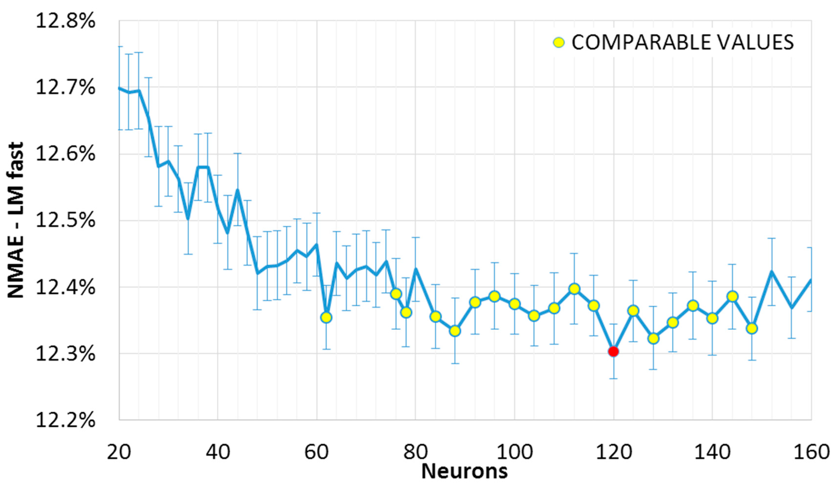
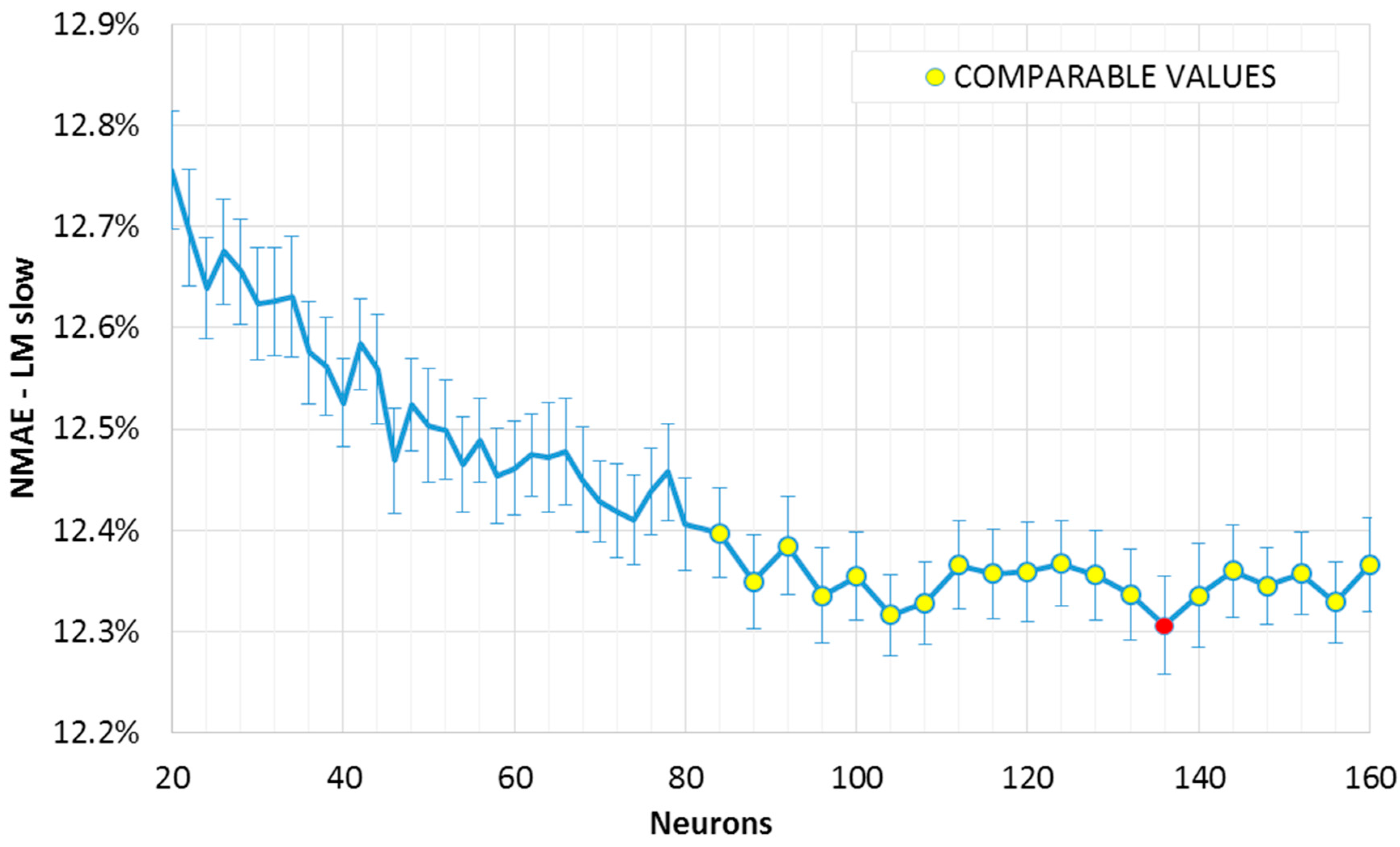
The results can be observed in the Figure 1 and Figure 2, where the mean NMAE% trend as a function of the neurons in the single hidden layer is shown. The error function reaches a minimum within a broad interval of neurons, after which it seems to increase again. This slight growth is not evident in the slow convergence algorithm (“LM slow”, Figure 2); however, we may expect that this will not decrease further, as the error has reached a minimum region. In fact, while an exact point for the minimum of the sample mean can be determined, (the red points in Figure 1 and Figure 2), this value is included in an interval of confidence. If such a range matches other minima (which are not necessarily adjacent), it would not be possible to exactly determine which one of the two points actually represents the absolute minimum (the “optimum” value). Two intervals of confidence are called “compatible” if their intersection is not null. The mean points representing intervals compatible with the minimum interval are shown in Figure 1 and Figure 2 (red point), and have been highlighted in yellow. It can be noted that, for the fast convergence algorithm (“LM fast”, Figure 1) with an equal number of similar networks, the trend is more variable: the higher variance generates wider intervals. As a consequence, we have a higher number of compatible points, and higher uncertainty in the optimum configuration.
It is useful to recall here that such intervals contain the real mean value within a 95% degree of confidence. It is then plausible to assume that some of these points are outliers (consider for example the value for 62 neurons in Figure 1). Indeed, the error variation within the optimal range is shown to be minimal in these graphs. Besides, it is better to consider also the error from the ensemble forecasting method as it is described in the following section. Looking at Figure 1 and Figure 2, a suitable number of neurons for a single layer FFNN is between 100 and 120, with a training-validation dataset composition as explained in Section 4.
The proposed approach provides generally good and flexible results on a whole year data basis, including all kinds of meteorological conditions. The daily errors in different weather conditions according to the presented methodology are variable, as already shown in [15]. The forecasting performances (as daily NMAE%) vary according to the weather conditions, as follows: around 2% for a sunny day; 7% for highly variable cloudy day; and 8% for a typical overcast day. The proposed PHANN approach has been already validated versus other methods for a day-ahead PV power forecasts in [33]: results obtained in a real application scenario, after setting neural network parameters with the here proposed methodology, have proved to reach lower error rates.
7. Number of Trials in the Ensemble Forecast
In order to obtain the lowest error, it is also worthwhile to estimate how many trials should be employed in the ensemble forecast. The improvement is expected to reach an asymptotic value with a growing number of trials; however, by increasing the amount of trials, the calculation time is enlarged. Therefore, there is a threshold gain between the number of trials and the reached improvement.
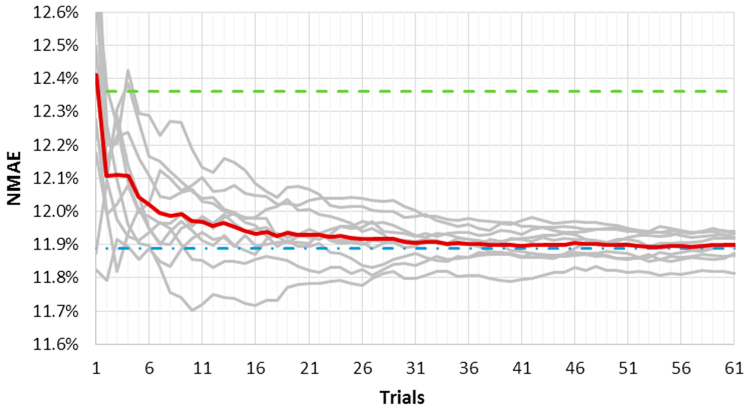
The procedure of looking for the minimum NMAE%, along with the amount of trials, is outlined as follows. The training Levenberg–Marquardt algorithms both with fast and slow convergence are adopted, and the ensemble forecast is performed by an ANN with 120 number of neurons. A growing number of trials were analyzed up to a maximum equal to one thousand.
First, the NMAE% is calculated for ten independent ensemble forecasts. The term “independent” means that different ensemble forecasts do not have common trials. The n-th ensemble forecast is performed by using a growing quantity of trials, starting from one trial and going up to one hundred trials, in order to infer the global trends of the ensemble NMAE%, while trying to avoid any possible random influence due to a few number of cases.
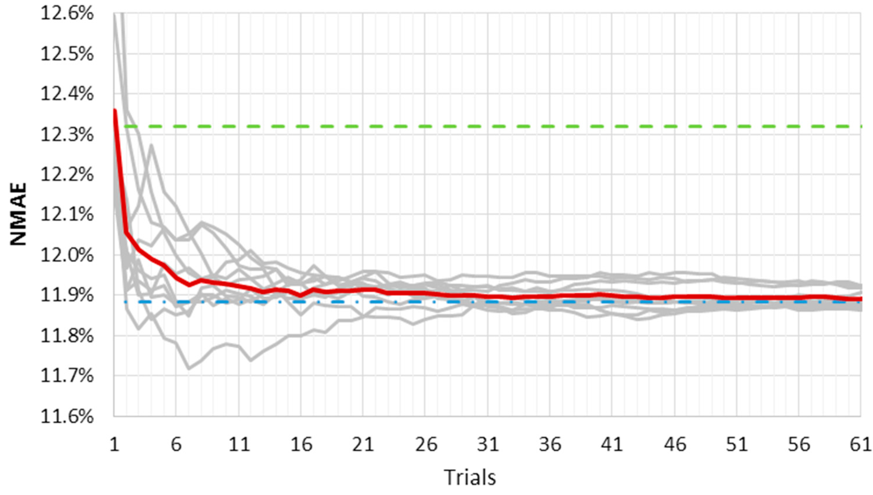
Figure 3 and Figure 4 show the results of this analysis for the LM fast and slow training algorithms, respectively. They represent the ten NMAE% error curves as a function of the average outputs number used for the ensemble method (grey lines). The mean NMAE% of the ten ensemble forecasts is depicted in red; the mean NMAE% of one thousand forecasts is the upper constant dashed green line; and the NMAE% of the ensemble forecast made by one thousand trials is the lower constant dash-dotted blue line. The red line represents a “trend index”, and it rapidly tends to an asymptotic value that can be considered “stable”.
It must be pointed out that as far as the number of trials gets close to one thousand, the red and the blue line will tend to coincide. However, the graphs have an upper limit equal to 100 trials in the x axis, as we consider ten independent ensembles from one thousand different forecasts.
When the slow convergence algorithm is used, such stability is reached for a smaller number of trials, as shown in Figure 4. Furthermore, the curves’ variability here is lower, reflecting the lower error variance of the output. Even the advantage initially offered by the fast convergence algorithm—that is, the short calculation time—seems now to be compensated for by the need of a lower number of outputs in the slow convergence algorithm. A larger number of forecasts in the ensemble method would slightly decrease NMAE%, which bears the brunt of a much higher computational burden.
8. Number of Neurons in a Dual Layer ANN
In this work, networks with two hidden layers between the input and the output have also been analyzed. This network topology has two degrees of freedom related to the optimum number of neurons. Therefore, different criteria can be adopted, such as keeping the number of neurons in one layer constant while varying them in the other, or keeping a constant ratio of neurons between the layers, etc. Several simulations have been performed, but hereafter only the Levenberg–Marquardt training algorithm with a slow convergence setting is considered.
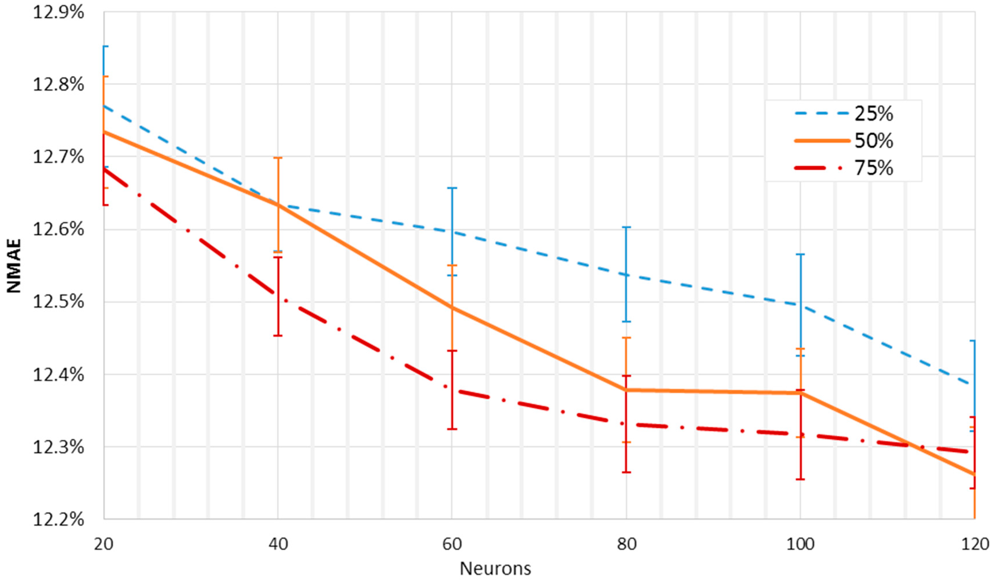
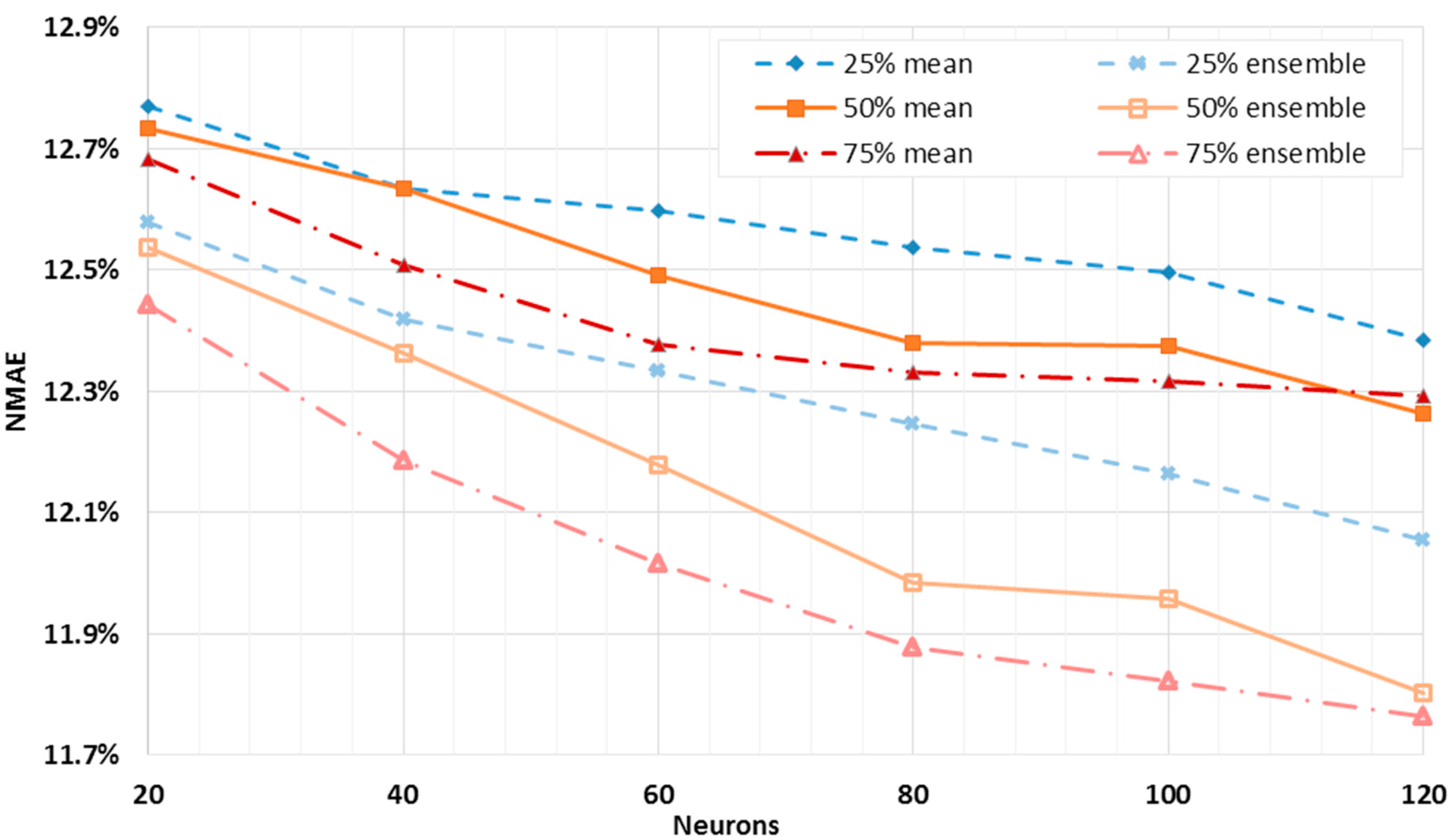
Figure 5 shows the mean NMAE% trends of the dual layer networks as a function of the neurons of the first layer, for a total of 50 forecasts for each layout. From 20 to 120 neurons were employed, with an increasing rate of 20 neurons. In Figure 6, the neurons of the second layer were fixed at 25%, 50%, and 75% of the first layer neurons, rounded up, and originating in this way three different curves. The best result is comparable to the one reached by the single layer networks. However, here it is possible, by analyzing the gradient of the orange curve, to have small margins of improvement while the number of neurons is increasing. Similarly to the analysis carried out for a single layer network, the NMAE% is calculated for the ensemble of the forecasts, and it is shown together with the mean error of the single outputs. Also in this case, the shape of the curves suggests looking for the optimum layout towards a higher number of neurons. Moreover, the smallest value of the error for the ensemble output is slightly less than the one obtained by the single layer networks. Therefore, the dual layer networks seem to provide better performance.
Although the dual layer networks seem to provide slightly better performance, single layer networks seem to be more appropriate for this kind of forecast. In fact, dual layer networks with larger numbers of neurons need remarkably higher calculation times, and this might represent a great drawback for their employment. As an example, the training of only one single layer network with 120 neurons required an average of 50 s, while the training of a unique dual layer network with 120 and 90 neurons required nearly 350 s on a quad-core Intel®, Santa Clara, CA, USA, CoreTM i7-2640M CPU, with an operating frequency of 2.8 GHz, and 8 GB ram.
9. Conclusions
This work has presented a detailed analysis of a method which has been defined for the setting up of an ANN in terms of number of trials in the ensemble forecast, the number of neurons, and their layout. This method has been employed for a day-ahead forecast with a recently developed PHANN approach.
On the basis of the proposed method, the settings minimizing the mean NMAE% of the 24 h ahead PV power forecast with a one-year historical dataset are: an ensemble size of ten trials, and a number of 120 neurons in a single layer ANN configuration. The above outlined method is meant to be adopted for setting the most suitable ANN parameters in view of the day-ahead forecast of any PV plant’s output power.
Author Contributions
In this research activity, all of the authors were involved in the data analysis and preprocessing phase, the simulation, the results analysis and discussion, and the manuscript’s preparation. All of the authors have approved the submitted manuscript. S.L. and M.M. conceived and designed the experiments; E.O. performed the experiments; E.O. and M.M. analyzed the data; F.G. contributed analysis tools; all the authors equally contributed to the writing of the paper.
Conflicts of Interest
The authors declare no conflict of interest.
References
- Brenna, M.; Dolara, A.; Foiadelli, F.; Lazaroiu, G.C.; Leva, S. Transient analysis of large scale PV systems with floating DC section. Energies 2012, 5, 3736–3752. [Google Scholar] [CrossRef]
- Paulescu, M.; Paulescu, E.; Gravila, P.; Badescu, V. Weather Modeling and Forecasting of PV Systems Operation; Green Energy Technology; Springer: London, UK, 2013. [Google Scholar]
- Omar, M.; Dolara, A.; Magistrati, G.; Mussetta, M.; Ogliari, E.; Viola, F. Day-ahead forecasting for photovoltaic power using artificial neural networks ensembles. In Proceedings of the 2016 IEEE International Conference on Renewable Energy Research and Applications (ICRERA), Birmingham, UK, 20–23 November 2016; pp. 1152–1157. [Google Scholar]
- Cali, Ü. Grid and Market Integration of Large-Scale Wind Farms Using Advanced Wind Power Forecasting: Technical and Energy Economic Aspects; Kassel University Press: Kassel, Germany, 2011. [Google Scholar]
- Gardner, M.; Dorling, S. Artificial neural networks (the multilayer perceptron)—A review of applications in the atmospheric sciences. Atmos. Environ. 1998, 32, 2627–2636. [Google Scholar] [CrossRef]
- Lippmann, R. An introduction to computing with neural nets. IEEE ASSP Mag. 1987, 4, 4–22. [Google Scholar] [CrossRef]
- Gandelli, A.; Grimaccia, F.; Leva, S.; Mussetta, M.; Ogliari, E. Hybrid model analysis and validation for PV energy production forecasting. In Proceedings of the International Joint Conference on Neural Networks, Beijing, China, 6–11 July 2014. [Google Scholar]
- Nelson, M.M.; Illingworth, W.T. A Practical Guide to Neural Nets; Addison-Wesley: Reading, MA, USA, 1991; Volume 1. [Google Scholar]
- Pelland, S.; Remund, J.; Kleissl, J.; Oozeki, T.; De Brabandere, K. Photovoltaic and Solar Forecasting: State of the Art. Int. Energy Agency Photovolt. Power Syst. Program. Rep. 2013, 14, 1–40. [Google Scholar]
- Jayaweera, D. Smart Power Systems and Renewable Energy System Integration; Springer International Publishing: Cham, Switzerland, 2016; Volume 57. [Google Scholar]
- Kalogirou, S.A. Artificial Intelligence in Energy and Renewable Energy Systems; Nova Science Publishers: Commack, NY, USA, 2006. [Google Scholar]
- Raza, M.Q.; Nadarajah, M.; Ekanayake, C. On recent advances in PV output power forecast. Sol. Energy 2016, 136, 125–144. [Google Scholar] [CrossRef]
- Li, G.; Shi, J.; Zhou, J. Bayesian adaptive combination of short-term wind speed forecasts from neural network models. Renew. Energy 2011, 36, 352–359. [Google Scholar] [CrossRef]
- Quan, D.M.; Ogliari, E.; Grimaccia, F.; Leva, S.; Mussetta, M. Hybrid model for hourly forecast of photovoltaic and wind power. In Proceedings of the IEEE International Conference on Fuzzy Systems, Hyderabad, India, 7–10 July 2013. [Google Scholar]
- Dolara, A.; Grimaccia, F.; Leva, S.; Mussetta, M.; Ogliari, E. A physical hybrid artificial neural network for short term forecasting of PV plant power output. Energies 2015, 8, 1138–1153. [Google Scholar] [CrossRef]
- Leva, S.; Dolara, A.; Grimaccia, F.; Mussetta, M.; Ogliari, E. Analysis and validation of 24 hours ahead neural network forecasting of photovoltaic output power. Math. Comput. Simul. 2017, 131, 88–100. [Google Scholar] [CrossRef]
- Ripley, B.D. Statistical Ideas for Selecting Network Architectures. In Neural Networks: Artificial Intelligence and Industrial Applications, Proceedings of the Third Annual SNN Symposium on Neural Networks, Nijmegen, The Netherlands, 14–15 September 1995; Kappen, B., Gielen, S., Eds.; Springer: London, UK; pp. 183–190.
- Benardos, P.G.; Vosniakos, G.-C. Optimizing feedforward artificial neural network architecture. Eng. Appl. Artif. Intell. 2007, 20, 365–382. [Google Scholar] [CrossRef]
- Basheer, I.; Hajmeer, M. Artificial neural networks: Fundamentals, computing, design, and application. J. Microbiol. Methods 2000, 43, 3–31. [Google Scholar] [CrossRef]
- Beale, M.H.; Hagan, M.T.; Demuth, H.B. Neural Network ToolboxTM User’s Guide; MathWorks Inc.: Natick, MA, USA, 1992. [Google Scholar]
- Widrow, B.; Lehr, M.A. 30 Years of Adaptive Neural Networks: Perceptron, Madaline, and Backpropagation. Proc. IEEE 1990, 78, 1415–1442. [Google Scholar] [CrossRef]
- Cover, T.M. Geometrical and Statistical Properties of Linear Threshold Devices; Department of Electrical Engineering, Stanford University: Stanford, CA, USA, 1964. [Google Scholar]
- Cover, T.M. Capacity problems for linear machines. Pattern Recognit. 1968, 283–289. [Google Scholar]
- Baum, E.B.; Haussler, D. What Size Net Gives Valid Generalization? Neural Comput. 1989, 1, 151–160. [Google Scholar] [CrossRef]
- Hertz, J.; Krogh, A.; Palmer, R.G. Introduction to the Theory of Neural Computation; Westview Press: Boulder, CO, USA, 1991; Volume 1. [Google Scholar]
- Grossman, T.; Meir, R.; Domany, E. Learning by Choice of Internal Representations. Complex Syst. 1989, 2, 555–575. [Google Scholar]
- Chow, S.K.H.; Lee, E.W.M.; Li, D.H.W. Short-term prediction of photovoltaic energy generation by intelligent approach. Energy Build. 2012, 55, 660–667. [Google Scholar] [CrossRef]
- Frederick, M. Neuroshell Manual; Ward Systems Group Inc.: Frederick, MD, USA, 1996; Volume 2. [Google Scholar]
- Mezard, M.; Nadal, J.-P. Learning in feedforward layered networks: The tiling algorithm. J. Phys. A Math. Gen. 1989, 22, 2191–2203. [Google Scholar] [CrossRef]
- Castellano, G.; Fanelli, A.M.; Pelillo, M. An iterative pruning algorithm for feedforward neural networks. IEEE Trans. Neural Netw. 1997, 8, 519–531. [Google Scholar] [CrossRef] [PubMed]
- Huang, S.-C.; Huang, Y.-F. Bounds on the number of hidden neurons in multilayer perceptrons. IEEE Trans. Neural Netw. 1991, 2, 47–55. [Google Scholar] [CrossRef] [PubMed]
- Shao, J. Fundamentals of Statistics. In Mathematical Statistics; Springer: New York, NY, USA, 2003; pp. 91–160. [Google Scholar]
- Ogliari, E.; Dolara, A.; Manzolini, G.; Leva, S. Physical and hybrid methods comparison for the day ahead PV output power forecast. Renew. Energy 2017, 113, 11–21. [Google Scholar] [CrossRef]
- Dolara, A.; Leva, S.; Mussetta, M.; Ogliari, E. PV hourly day-ahead power forecasting in a micro grid context. In Proceedings of the EEEIC 2016—International Conference on Environment and Electrical Engineering, Florence, Italy, 6–8 June 2016. [Google Scholar]
Figure 1.
Mean normalized mean absolute error (NMAE%) as a function of the number of neurons, with Levenberg–Marquardt training algorithm set for a faster convergence. Comparable mean NMAE% in yellow, with 95% interval of confidence, with the minimum in red.
Figure 1.
Mean normalized mean absolute error (NMAE%) as a function of the number of neurons, with Levenberg–Marquardt training algorithm set for a faster convergence. Comparable mean NMAE% in yellow, with 95% interval of confidence, with the minimum in red.

Figure 2.
Mean NMAE% as a function of the number of neurons, with Levenberg–Marquardt training algorithm set for a slower convergence. Comparable mean NMAE% in yellow, with 95% interval of confidence, with the minimum in red.
Figure 2.
Mean NMAE% as a function of the number of neurons, with Levenberg–Marquardt training algorithm set for a slower convergence. Comparable mean NMAE% in yellow, with 95% interval of confidence, with the minimum in red.

Figure 3.
NMAE% of ten random ensemble (grey lines) as a function of the growing number of trials. The artificial neural network (ANN) has 120 neurons and an “LM fast” training algorithm. The mean of the ten ensemble forecasts is in red, the mean NMAE% of one thousand forecasts is the dashed green line, and the ensemble NMAE% of one thousand forecasts is the dash-dotted blue line.

Figure 4.
NMAE% of ten random ensemble (grey lines) as a function of the growing number of trials. The artificial neural network (ANN) has 120 neurons and a “Levenberg–Marquardt (LM) slow” training algorithm. The mean of the ten ensemble forecasts is in red, the mean of one thousand forecasts is the dashed green line, and the ensemble NMAE% of one thousand forecasts is the dash-dotted blue line.

Figure 5.
Mean NMAE% of 50 different forecasts as a function of the hidden layers’ sizes, with a constant ratio of neurons.
Figure 5.
Mean NMAE% of 50 different forecasts as a function of the hidden layers’ sizes, with a constant ratio of neurons.

Figure 6.
Comparison between the mean NMAE% and the ensemble NMAE% of 50 trials as a function of the hidden layers’ sizes, kept with a constant ratio of neurons.
Figure 6.
Comparison between the mean NMAE% and the ensemble NMAE% of 50 trials as a function of the hidden layers’ sizes, kept with a constant ratio of neurons.


Table 1.
Levenberg–Marquardt (LM) training algorithm settings.
| Settings | LM Fast (Default) | LM Slow |
|---|---|---|
| ω | 10−3 | 1 |
| δ | 10 | 2 |
| Φ | 10−1 | −0.5 |
© 2017 by the authors. Licensee MDPI, Basel, Switzerland. This article is an open access article distributed under the terms and conditions of the Creative Commons Attribution (CC BY) license (http://creativecommons.org/licenses/by/4.0/).
Share and Cite
MDPI and ACS Style
Grimaccia, F.; Leva, S.; Mussetta, M.; Ogliari, E. ANN Sizing Procedure for the Day-Ahead Output Power Forecast of a PV Plant. Appl. Sci. 2017, 7, 622. https://0-doi-org.brum.beds.ac.uk/10.3390/app7060622
AMA Style
Grimaccia F, Leva S, Mussetta M, Ogliari E. ANN Sizing Procedure for the Day-Ahead Output Power Forecast of a PV Plant. Applied Sciences. 2017; 7(6):622. https://0-doi-org.brum.beds.ac.uk/10.3390/app7060622
Chicago/Turabian StyleGrimaccia, Francesco, Sonia Leva, Marco Mussetta, and Emanuele Ogliari. 2017. "ANN Sizing Procedure for the Day-Ahead Output Power Forecast of a PV Plant" Applied Sciences 7, no. 6: 622. https://0-doi-org.brum.beds.ac.uk/10.3390/app7060622
Note that from the first issue of 2016, this journal uses article numbers instead of page numbers. See further details here.