
Combined CFD-Stochastic Analysis of an Active Fluidic Injection System for Jet Noise Reduction

1
Department of Air Transport Environmental Impact, Italian Aerospace Research Center (CIRA), 81043 Capua, Italy
2
Department of Industrial Engineering, University of Naples “Federico II”, 80138 Naples, Italy
*
Author to whom correspondence should be addressed.
Appl. Sci. 2017, 7(6), 623; https://0-doi-org.brum.beds.ac.uk/10.3390/app7060623
Submission received: 3 May 2017
/
Revised: 13 June 2017
/
Accepted: 14 June 2017
/
Published: 16 June 2017
(This article belongs to the Special Issue Advances in Vibroacoustics and Aeroacustics of Aerospace and Automotive Systems)
Abstract
:In the framework of DANTE project (Development of Aero-Vibroacoustics Numerical and Technical Expertise), funded under the Italian Aerospace Research Program (PRORA), the prediction and reduction of noise from subsonic jets through the reconstruction of turbulent fields from Reynolds Averaged Navier Stokes (RANS) calculations are addressed. This approach, known as Stochastic Noise Generation and Radiation (SNGR), reconstructs the turbulent velocity fluctuations by RANS fields and calculates the source terms of Vortex Sound acoustic analogy. In the first part of this work, numerical and experimental jet-noise test cases have been reproduced by means RANS simulations and with different turbulence models in order to validate the approach for its subsequent use as a design tool. The noise spectra, predicted with SNGR, are in good agreement with both the experimental data and the results of Large-Eddy Simulations (LES). In the last part of this work, an active fluid injection technique, based on extractions from turbine and injections of high-pressure gas into the main stream of exhausts, has been proposed and finally assessed with the aim of reducing the jet-noise through the mixing and breaking of the turbulent eddies. Some tests have been carried out in order to set the best design parameters in terms of mass flow rate and injection velocity and to design the system functionalities. The SNGR method is, therefore, suitable to be used for the early design phase of jet-noise reduction technologies and a right combination of the fluid injection design parameters allows for a reduction of the jet-noise to 3.5 dB, as compared to the baseline case without injections.
1. Introduction
The problem of noise generation by compressible turbulent jets has been the subject of studies since the early 1950s, with the introduction of the turbojet also in commercial aircraft. It has continued, even later since the 1980s, with the introduction of turbofan with high bypass ratios, inherently less noisy than previously, due to the reduced exhaust velocity. In recent decades, the problem of jet noise prediction has been numerically addressed through a broad range of methods.
Despite the application of Direct Numerical Simulation (DNS) to jet-noise prediction [1,2,3,4], becoming more feasible with the growing advancement in computational resources, due to the large disparities of length and energy scales between fluid and acoustic fields, the use of fully solved Navier Stokes equations without turbulence modeling (DNS) is still restricted to low Reynolds number flows.
Instead, the numerical simulation of aeroacoustics through the solution of filtered Navier Stokes equations, either using fully Large Eddy Simulation (LES) or hybrid Reynolds Averaged Navier Stokes-LES approaches, such as the detached eddy simulation (DES), is a major area of research [5,6,7]. However, despite the increase in computational power, even these types of simulations are not yet feasible for industrial purposes. Indeed, industry interest is mainly devoted to reliable numerical tools to be applied to realistic configurations for redesign of old configurations and for the development of new technologies. Furthermore, the growing interest on multi-disciplinary and multi-objective optimization necessarily lead to approaches that require low computational time.
Therefore, Reynolds Averaged Navier Stokes (RANS) simulations still remains the more feasible approach for Computational Fluid Dynamics (CFD) applications of industrial interest. However, RANS computations are not able to model, solely, the aeroacoustic phenomena. In this context, the stochastic approach for the prediction of noise from turbulence has received a great deal of interest in recent years. It was introduced by Kraichnan [8] and Fung [9], and it is based on the idea that Fourier components of solenoidal velocity fluctuations can be sampled in the wave-number space from a prescribed mono-dimensional energy spectrum. The revision and improvement of these methods for aeroacoustic applications have produced the stochastic noise generation and radiation (SNGR) methods [10,11,12,13,14,15].
Concerning the jet-noise reduction devices, in recent decades, chevron nozzles attracted much attention to their noise reduction benefits and are currently one of the most popular jet-noise reduction devices. Chevrons typically reduce low frequency noise, while increasing high frequency noise [16] with a limited thrust loss of only about 0.25%. Downstream vortex, generated by chevron, improves mixing in the shear layer, which leads to a decrease or increase in noise at certain frequency ranges. Several RANS computational studies were conducted about chevron nozzles [17,18,19]. The first LES calculations for the chevron nozzle jets appeared to be performed by Shur et al. [20,21].
A promising technology seems to be the fluidic chevron, as alternative solution to the mechanical chevron. This device consists of small injectors that inject high pressure air or other fluids, such as water, near the nozzle exit edge in order to emulate the mixing and the noise reduction features of the mechanical chevron. Numerous studies and experiments have been carried out to develop fluid chevron technology, especially at NASA Langley Jet Noise lab [22,23,24]. Fluidic chevrons, tested at NASA, were the first of their kind, designed with small slots near the nozzle exit edge to allow air injection into the stream and promote mixing between the core flow and the flow from the fan. Despite the simplicity of the mechanical chevron, the fluidic injection technique allows a greater flexibility. It can be used when the jet-noise reduction requirement is needed, for example during take-off and landing phases.
The main goal of this paper is two-fold. The first one is to make the assessment of an improved SNGR method based on the previous works of Casalino and Barbarino [13] and Di Francescantonio [14] through the comparison with experimental and LES data of a cold subsonic jet [7]. The second one is to assess the design of an active fluid injection technique, based on extractions from turbine and injections of high-pressure gas into the main stream of exhausts. The novelty of this paper is the proof of the potential of the SNGR approach as applied to the design of new devices suitable for jet noise reduction.
2. Model Description and Validation
2.1. Model Description
The SNGR approach assumes that the turbulent velocity field can be reconstructed as a summation of Fourier components, according to Kraichnan [8]. Therefore, the reconstructed turbulent velocity u′ at point x and time t reads:
where , and are the magnitude, phase and direction of the nth Fourier component, respectively.
As proposed by Bailly and Juvé [11], each Fourier mode is supposed to be convected at the local mean-flow velocity corrected by the vortex convection velocity ratio . This factor may account for the wall induction effect that reduces the vortex convection velocity with respect to the mean-flow velocity at the location of the vortex core. The factor may also account for the vertical induction in a jet shear layer, but this effect is negligible for low-speed subsonic jets. For jet noise prediction, the value has been used. Notice that the scalar product accounts for the local time variation of the velocity field. Assuming incompressibility, the zero-divergence condition, applied to the Equation (1), results in the relationship , stating that the wave vector is perpendicular to the velocity vector.
By supposing that the turbulent flow field is isotropic, the magnitude of the nth Fourier mode is related to the mono-dimensional energy spectrum E(k) by the expression, , where and are the wave number and the corresponding band of the n-th mode. The Von Kármán—Pao isotropic turbulence spectrum is assumed [10]; that is:
where K is the turbulent kinetic energy, A is a numerical constant, is the wave number of maximum energy, is the Kolmogorov wave number, is the kinematical viscosity of the fluid and is the turbulent dissipation rate.
The constants A and can be determined by equating the integral energy and the integral length scale derived from turbulence spectrum to the RANS quantities K and , respectively, being the isotropic turbulent velocity and the first tuning parameter of the method. The aforementioned calculation provides [11] and .
The parameter allows tuning of the RANS turbulent integral length scale of the large-scale eddies. Its value is, by definition, close to unity, but its optimal value depends on the turbulent flow structure and conditions and on the RANS turbulence model. The optimal value of the parameter was found by Casalino and Barbarino [13], and used in this work.
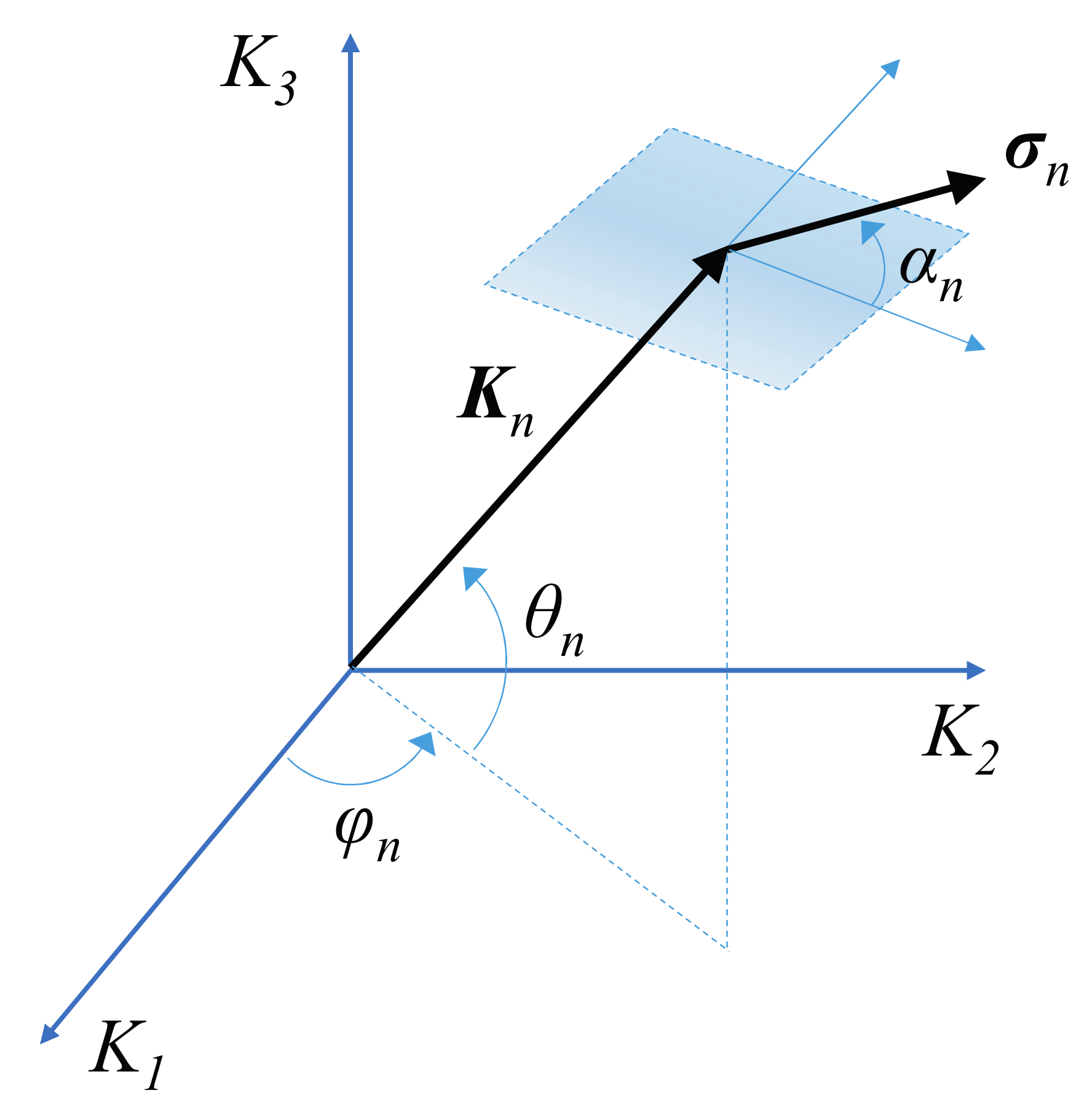
The stochastic isotropic and homogeneous velocity perturbation field can be generated by choosing probability density functions for all the random variables involved in the Fourier decomposition [10]. These random variables are the angles , , which define the direction of the wave vector , as sketched in Figure 1, the angle , which defines the direction of the unit vector in a plane orthogonal to , and finally the phase angle .
The requirement that the wave vector is uniformly distributed in the 3D wave-number space provides the following probability densities:
Analogously, by supposing that the vector is uniformly distributed in the plane normal to yields:
Finally, the phase angle is also supposed to be uniformly distributed in the 2π range, that is:
The extremes of the wave number interval are related, at each node of the CFD mesh, to the value of the wave number through the relationships:
where is the maximum distance between node i and its neighboring stencil nodes j, projected in the direction of the local mean-flow velocity ; is the number of grid points for the Fourier component, set to 6 in the present work, as suggested by Bailly and Juvé [11]. The optimal value of the Fourier modes number, , was found by Casalino and Barbarino [13], and used in this work. The constants and are two additional tuning constants of the stochastic model: , .
The use of an adaptive wave-number interval allows reducing the number of Fourier modes. Furthermore, in order to obtain a better discretization of the energy spectrum at the lower energy-containing Fourier modes, a logarithmic distribution of the values is used, say:
The energy spectrum is integrated over each band n to obtain the magnitude of the velocity component by discretizing the interval D in a number of constant subintervals, from the value up to the value .
A crucial point of the SNGR approach is the definition of the two-point space correlation of the velocity fluctuations at each node of the CFD mesh by means of an artificial numerical approach able to reproduce the physical behaviour of the turbulent structures. The simplest approach, used for instance in Bechara [10], would consist of segmenting the bounding box of the active source region in square paths with edges equal to the average value of the correlation length over the whole source region. Then, a set of stochastic angles are sampled in each patch and these values are finally attributed to all the mesh nodes falling in the patch. The main drawback of this approach is that the correlation length is the same over all the source region, and therefore, does not account for the local Reynolds stresses and size of the turbulent structures.
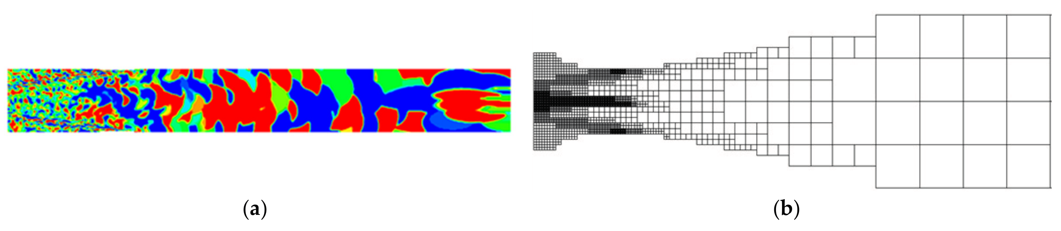
Conversely, two different SNGR approaches, based on the the correlation length of the CFD solution, have been proposed. The first one consists in dividing the domain in blobs whose dimension is proportional to the correlation length of the CFD cells falling inside the blob. In the first step, the RANS correlation lengths along the three Cartesian directions, each one denoted by the subscript k, are evaluated at each node, i, of the CFD mesh. Thus, random angles are assigned constant for each blob [13] as depicted in Figure 2a. The second one consists in projecting the CFD solution on an acoustic domain made of Cartesian cells whose dimension is proportional to the turbulent scale length of the CFD cells falling inside the acoustic Cartesian cell (Figure 2b). The correlation length is assumed to be different for each Fourier mode of Equation (1) and proportional to the mode wavelength, where is the wavelength of each Fourier mode [14]. For each mode, random angles are assigned constant for the acoustic Cartesian cells having the same correlation length.
The CFD mesh, used in the first approach, is not isotropic because its cells are elongated. Therefore, the CFD solution must be projected on a hexahedral mesh with uniform cells, which greatly increases the number of sources and consequently also computational time and memory.
Conversely, the second approach uses an adaptive acoustic mesh, wherein the cell size is representative of the turbulent vortex size: within the stream there are small cells in correspondence of small vortices and there are large cells in correspondence of large vortices. This adaptive acoustic mesh is isotropic, i.e., its cells have the same dimensions in all three directions, but at the same time it is also variable, i.e., locally, cells size is proportional to the turbulent vortex length.
The main advantage of the second approach is the reduction of the total cells to be processed in respect of the CFD mesh, reducing computation time and memory but ensuring the required refinement.
The computed velocity field is finally transformed in the frequency domain and assemble to compute the frequency counter-part of the Lamb vector .
According to the vortex sound analogy, the far field noise is finally achieved by the Powell’s equation in frequency domain:
where G is the free-field Green function and is the frequency counter-part of the Lamb vector.
2.2. Model Validation
The SNGR approach has been firstly validated against experimental and LES results of a subsonic jet with diameter , Mach number and the Reynolds number, , described by Andersson [7].
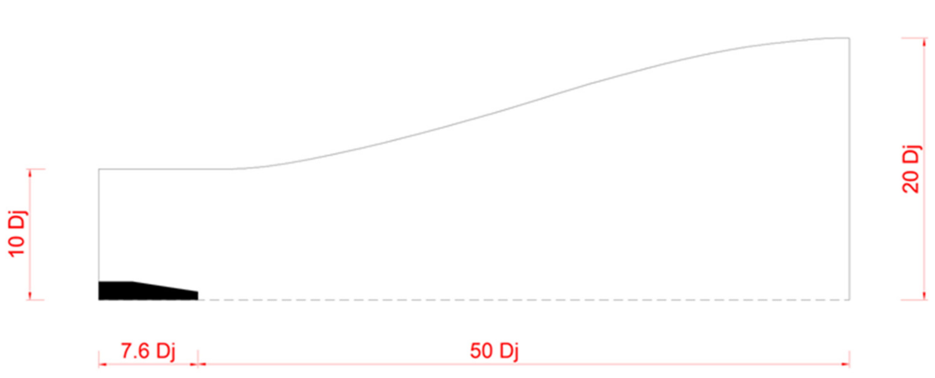
The two-dimensional geometry of the domain, shown in Figure 3, has been built using the CAD software Workbench by ANSYS.
A CFD RANS simulation based on the nozzle geometry used for the LES simulation [7] has been performed. The external profile of the nozzle has been reproduced by scanning from the original work [7]. The RANS simulation of the subsonic jet has been performed in the cold conditions, for which , where is the static temperature of the jet at the nozzle outlet section, and is the ambient temperature. In this study, the static temperature and pressure of the jet at the nozzle outlet section are respectively and . The temperature and pressure at the nozzle inlet section, respectively and , were calculated using Rankine Hugoniot equations:
where is the Mach Number while is the specific heat ratio of air, temperature and pressure at the nozzle inlet section, obtained by solving these two equations, are and .
The jet flow simulation has been carried out using the CFD software Fluent by ANSYS. The mesh extends from 0 to 50 nozzle diameters, , in the axial direction. The radial extension is at the nozzle outlet position and it increases up to at the far-field outlet position. Mesh cells are refined in the region near the nozzle exit and in the jet shear layer.
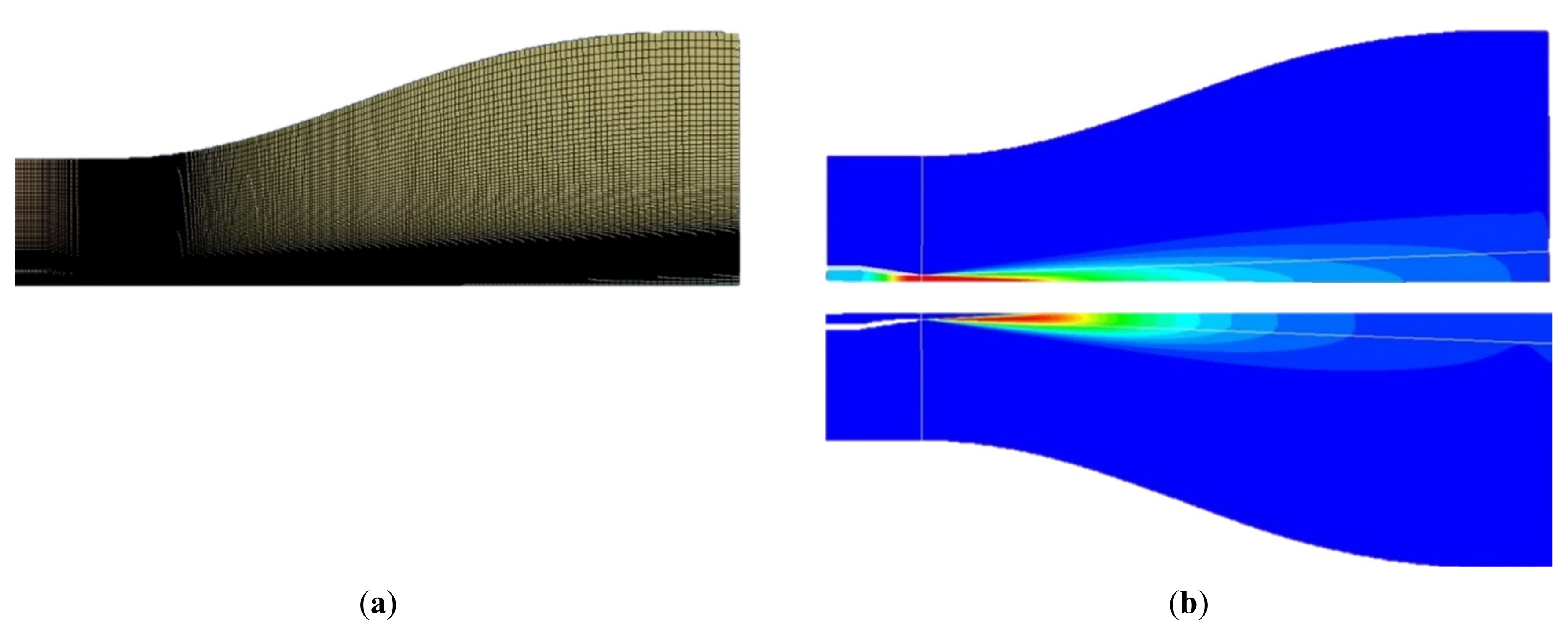
A 2D axisymmetric transient pressure based second-order upwind scheme has been employed to converge fully coupled RANS equations with turbulence accounted for through K-ε and K-ω SST models. A view of the mesh made up of cells and contour plots of the axial velocity and turbulent kinetic energy are shown in Figure 4.
The aerodynamic field results were extracted along the centerline and along radial lines at three axial positions downstream of the nozzle exit, according to Figure 5.
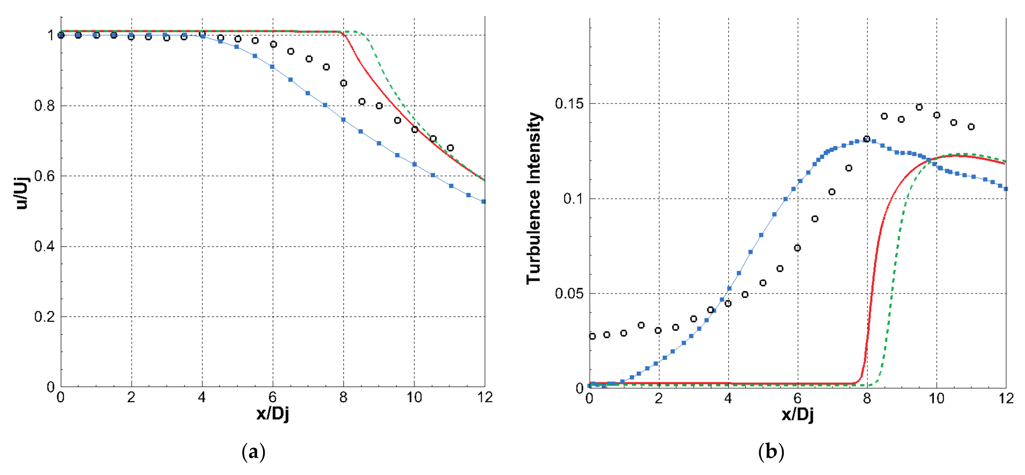
The laminar core and the decay of the centerline velocity are in good agreement with the experimental results. The predicted laminar core length of is slight higher than the experimental value as usual for RANS computations (Figure 6a). The maximum of centerline turbulent kinetic velocity occurs at about , in accordance with experimental results but its amplitude is slightly underestimated (Figure 6b).
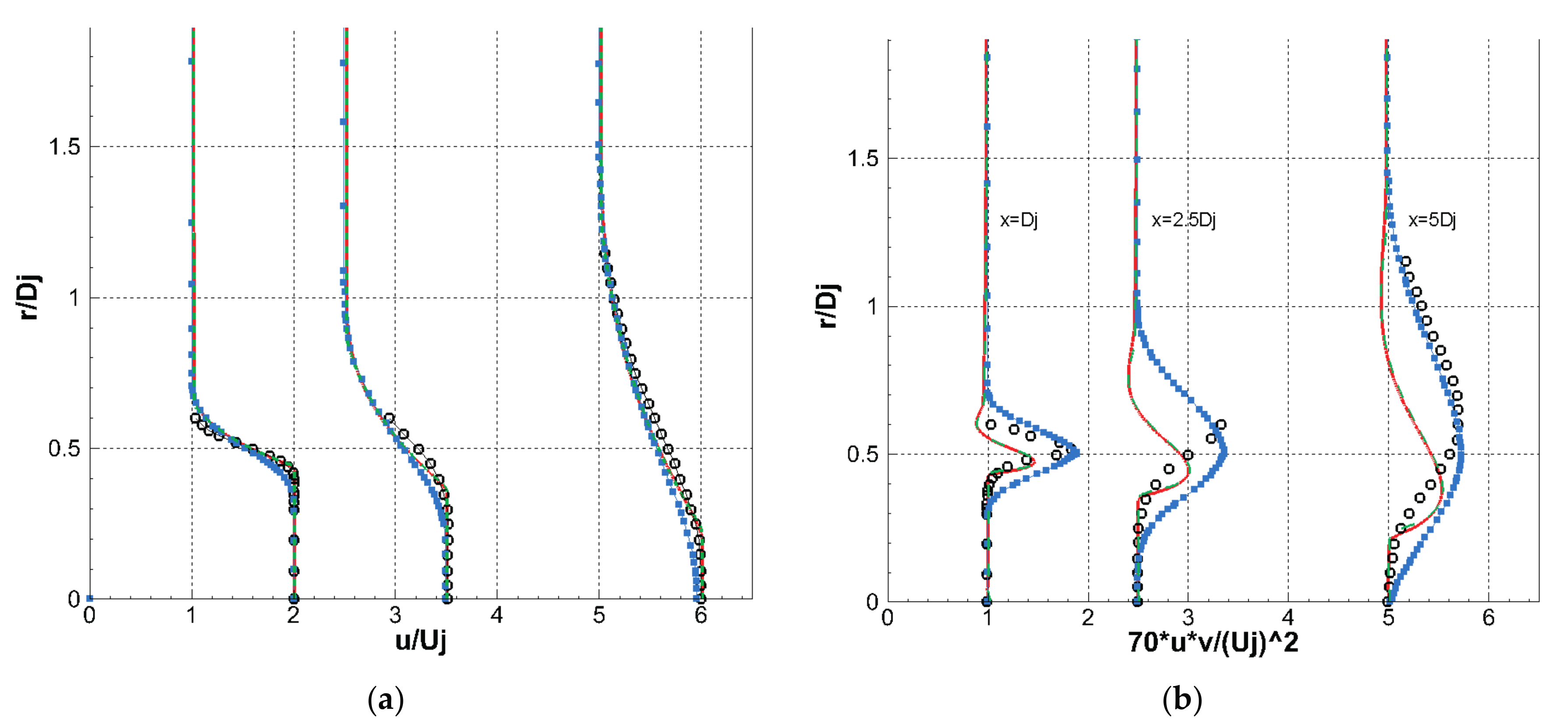
Moreover, the radial profile of the axial velocity is well predicted by both RANS and LES computations (Figure 7a), whereas, the uv correlation levels of the radial velocity profile are underestimated by the RANS analysis due to lower mixing predicted and overestimated by the LES (Figure 7b).
It can be argued that the RANS analysis results are in fairly good agreement with experimental data and LES results although they underestimate the value of uv correlation and do not predict the gradual increase of turbulent energy in the region of the laminar core.
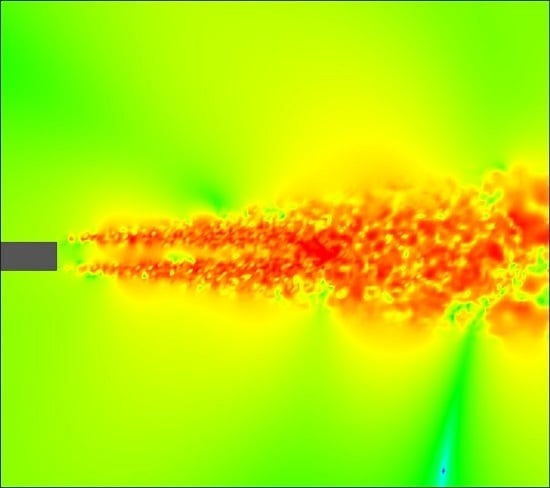
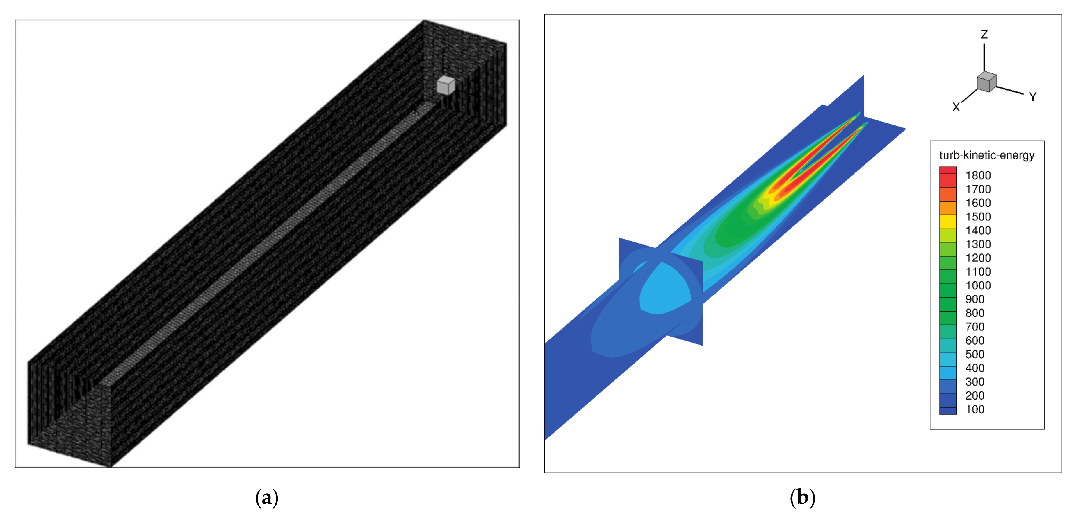
The acoustic field is evaluated by processing the RANS data by means the SNGR approach. To compute the stochastic noise sources, the axisymmetric CFD solution has been initially projected on a 3D domain, i.e., a uniform grid that consists of cubic cells with (Figure 8).
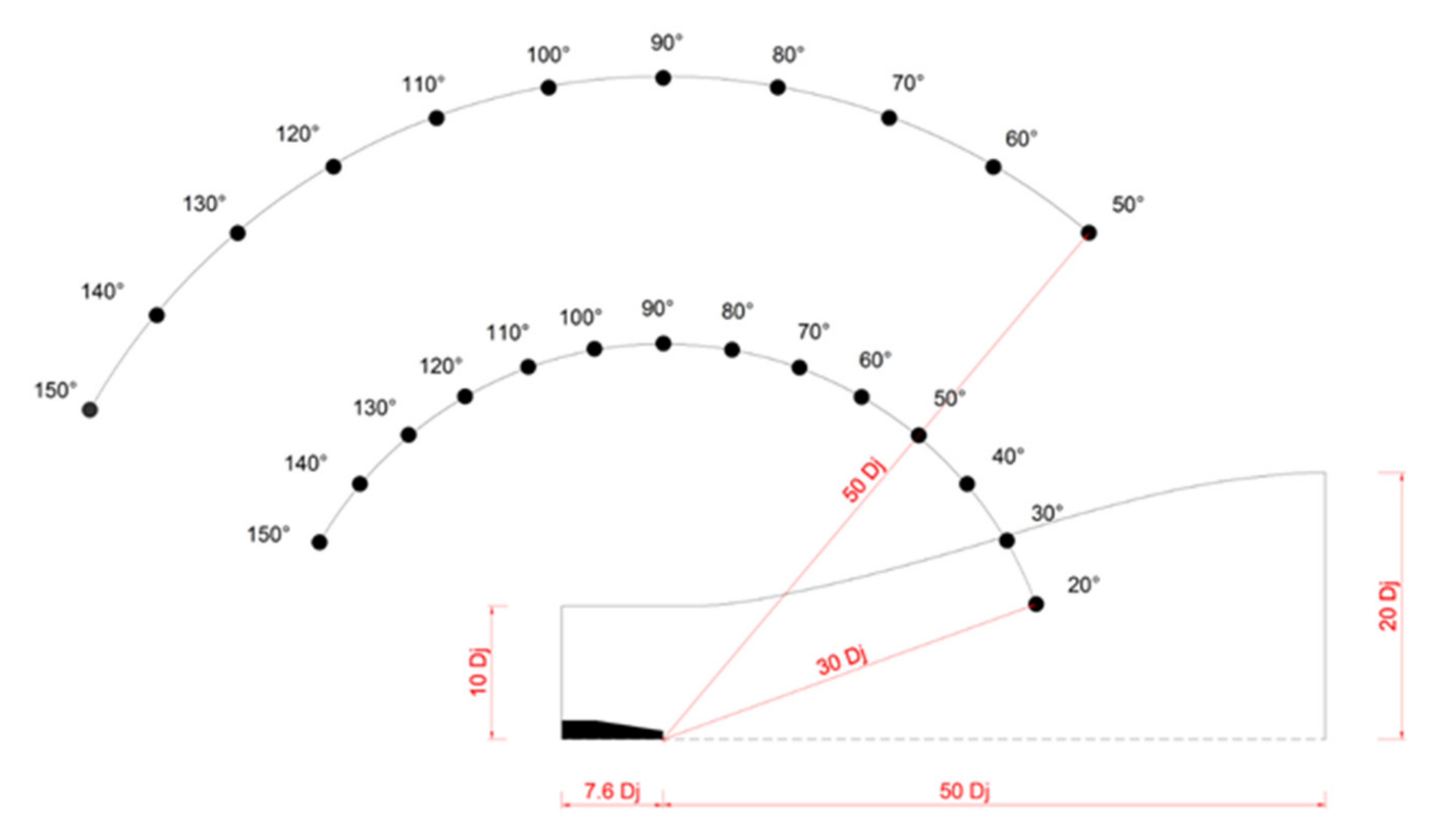
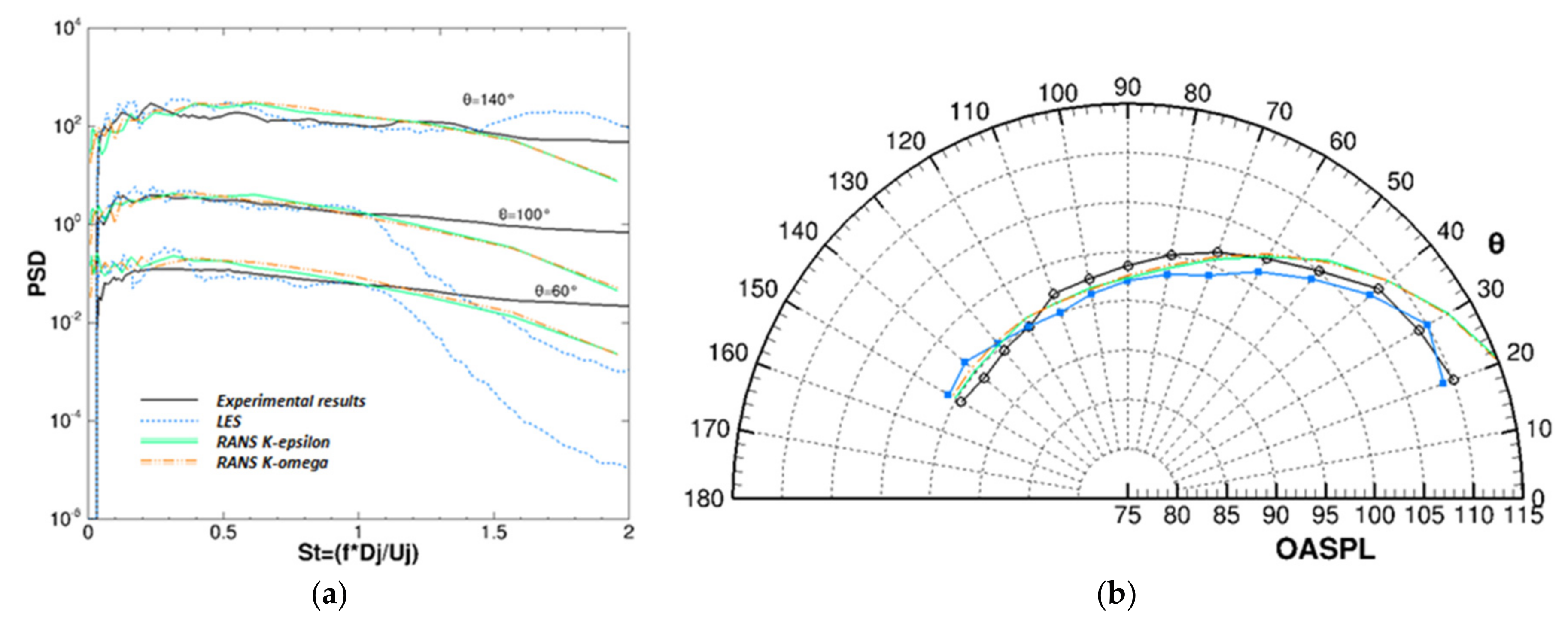
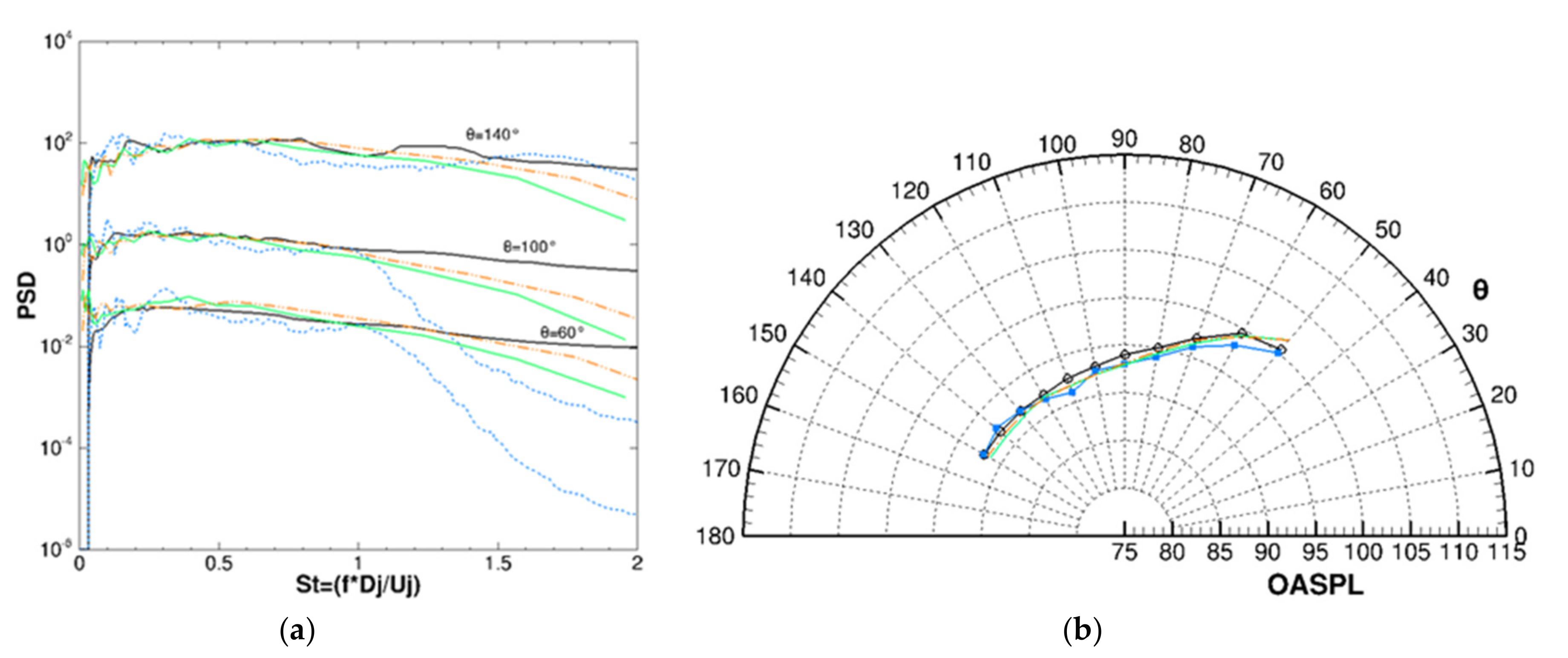
The noise has been computed directly from the Fourier transform of the Lamb vector by using the integral solution of Powell′s equation. Acoustic results are computed on a total of 25 microphones on two microphones arcs in the jet far-field region (Figure 9) and compared against LES and experimental results. Then, 14 microphones are arranged on a first arc of radius from the center of the nozzle outlet section and positioned by 20 degrees to 150 degrees with an angular step of 10 degrees. The remaining 11 microphones were placed on a second arc of radius from the center of the nozzle outlet section and positioned by 50 degrees to 150 degrees with an angular step of 10 degrees.
The acoustic results are expressed in terms of the PSD (Power Spectral Density) and OASPL (Over-All Sound Pressure Level).
To simplify the comparison with experimental data, the PSD spectra were filtered in third-octave bands. To represent all on the same graph, the PSD spectra have been staggered by multiplying the amplitude by a factor , where and being the angle from the jet axis.
SNGR method does not take account for either convective effects or refractions by the shear layer. Therefore, SNGR results have been corrected, as suggested by Lighthill [15], to account for convective effects by using a Doppler factor of , where is a proper exponential coefficient and is the convective Mach number. Furthermore, in a first approximation, mean flow refraction effects have been neglected.
Figure 10 and Figure 11 depict acoustic results for both arcs in terms of PSD spectra and OASPL levels showing that SNGR results are in very good agreement with the experimental results and LES analyses, with a matching within 2 dB except at the smaller angles where the maximum discrepancy is of about 5 dB (Figure 10b). In particular, the SNGR method allows predicting the trend of PSD spectra over a large part of the frequency range and up to . Instead, the LES method allows a good prediction only up to ; after that, the PSD spectra decay abruptly because of sub-grid filter that does not resolve the smallest scales, i.e., at the high frequencies. There are not great differences between the two models of turbulence, K-ε and K-ω SST.
In conclusion, the SNGR model, appropriately corrected by the Doppler factor, allows predicting the acoustic field of a subsonic jet both in terms of PSD spectra and in terms of directivity. In addition, the method is not very sensitive to the turbulence model adopted and allows estimating the jet-noise in a wide range of frequencies from a 2D axisymmetric RANS solution with a margin of uncertainty comparable to that of a LES calculation.
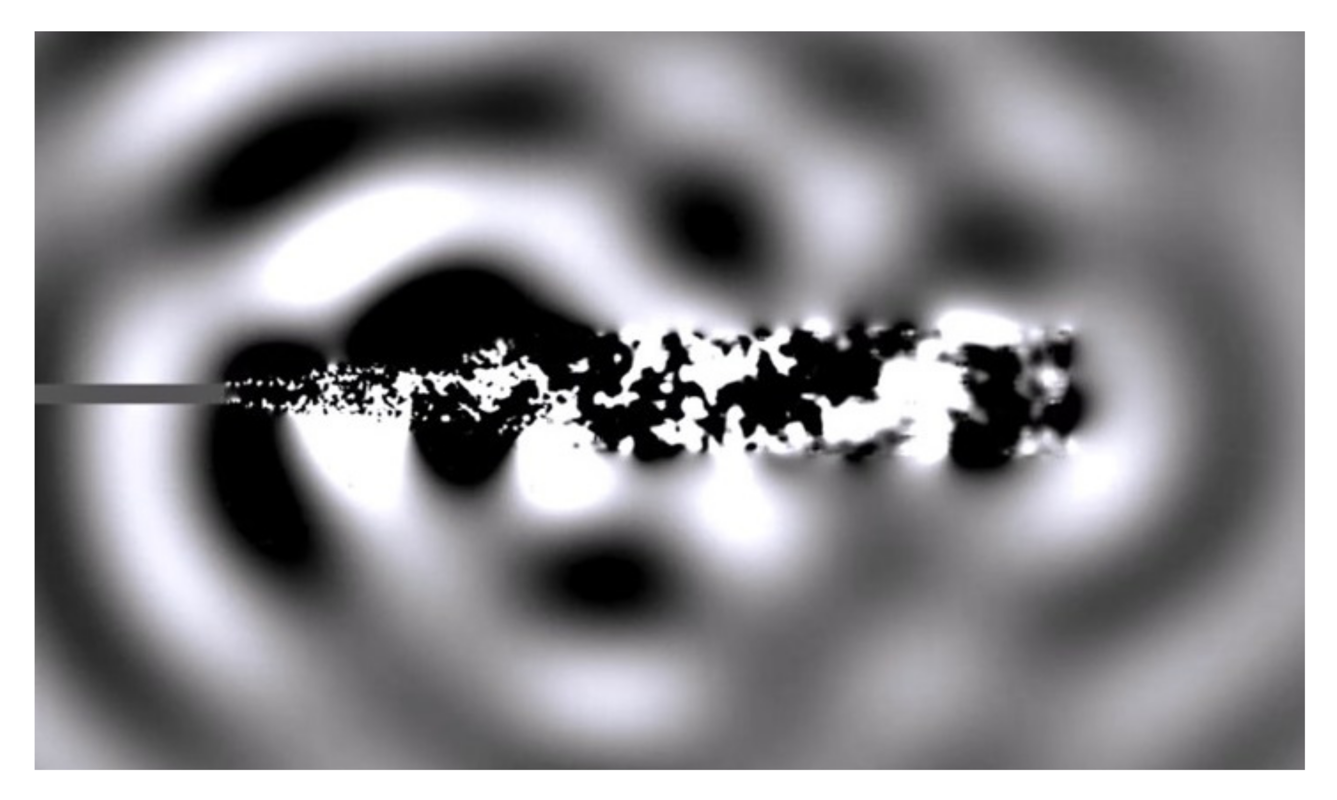
Finally, the contour plot of the real part of the acoustic pressure at 700 Hz and computed with the SNGR approach is shown in Figure 12. It can be observed that the lamb vector reconstructs the acoustic source encapsulated inside the jet flow region whereas the acoustic pressure propagates outside the jet region.
3. Active Fluidic Injection System
In this section, an experimental technology for reducing the jet noise based on a fluidic injection is assessed by means of the SNGR approach and applied to the jet analyzed in the Section 2.2. Several experimental studies, conducted over recent decades, have shown that the fluid injection technique effectively allows reduction of the noise from turbulence [22,23,24]. Therefore, the technological solution proposed here consists of injecting a small jet of secondary gas into the main flow, which comes out from the nozzle of the jet engine exhausts (Figure 13). This secondary jet is derived from gas bleeding from the turbine located immediately upstream of the nozzle.
The air extractions from the turbine and subsequent injections in the main stream of the exhaust gas at nozzle outlet favor a greater mixing in order to break the large turbulent structures at low frequencies, which are the main responsible for most of the radiated noise (Figure 14).
Figure 15 shows the difference in the view of the exhaust plume emitted from a jet engine between the cases with and without fluid injection.
In this work, four experimental tests were carried out to evaluate the influence of the bled mass flow rate, the area of the injection section and the jet angle over the noise reduction.
Two injection mass flow rate values are considered and corresponding about 5% and 10% of the total mass flow rate of the turbine. A maximum rate of about 10% has been used in order to preserve the nominal turbine power, whereas, pressure and temperature of the drained mass flow rate have been computed, assuming to be greater than the ambient conditions and according to the thermodynamic expansion. Two injection sections with a total area of around 4% and 10% of the nozzle outlet area have been considered and modelled in the computational domain and corresponding respectively to the 5% and 10% of the turbine mass flow rate. Finally, the spray conditions have been evaluated at three different injections angles equal to 45, 60 and 80 degrees.
The following test matrix (Table 1) has been, thus, assembled for the RANS + SNGR analyses. Examples of the different turbulence levels obtained by varying the injection patterns are displayed in Figure 16.
About the aerodynamic field results, Figure 17a shows the centerline profiles of the axial velocity obtained from four tests with injection. Increasing the jet angle, the predicted laminar core length decreases compared to the baseline case. In particular, focusing on the results of 3rd and 4th tests, the laminar core length of 4th test is greater than the 3rd one, because at the same jet angle, γ = 80°, the injected jet has a higher speed, due to the lower injection section area. At the same time, increasing the jet angle, the intensity of turbulence profiles moves toward the nozzle exit, because the mixing is locally increasing (Figure 17b).
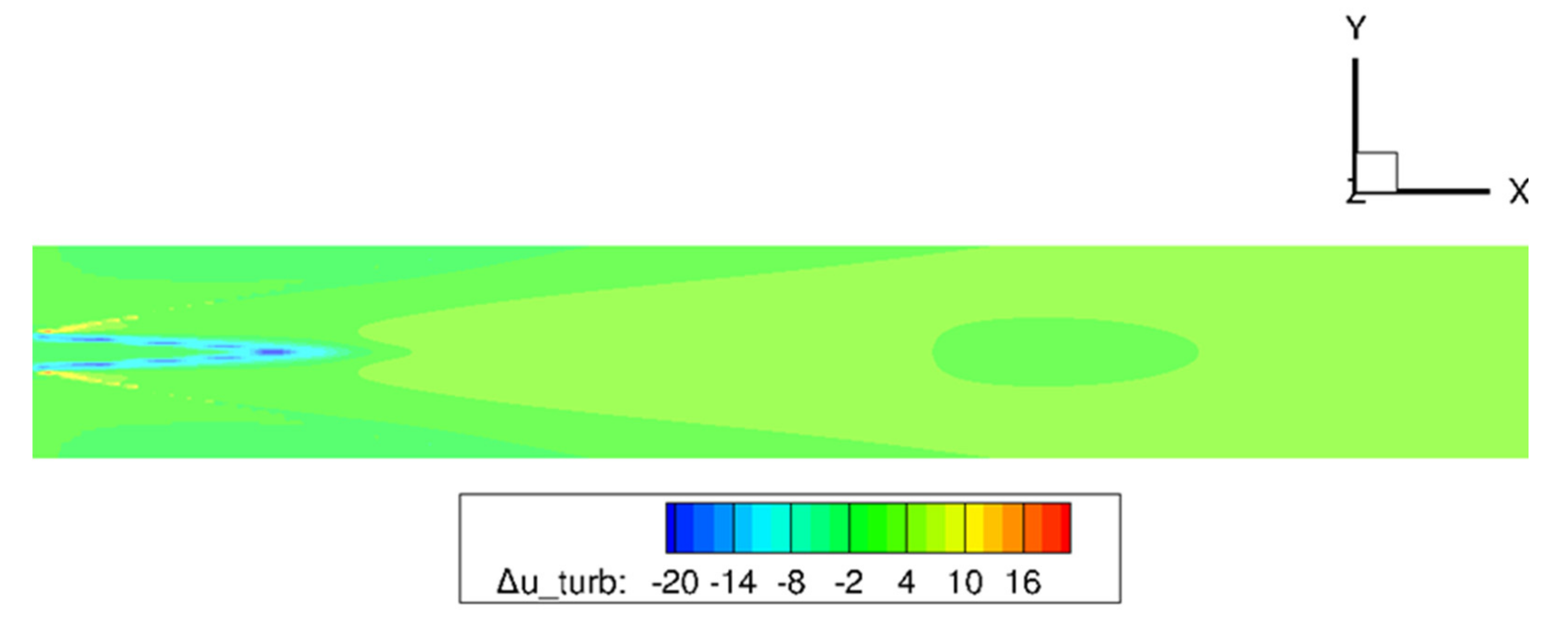
Figure 18 shows turbulent velocity difference, Δ𝑢𝑡𝑢𝑟𝑏, between the baseline case and the 4th test in the whole domain of interest. In the case with fluid injection, the impact between the injected jet and the main flow cause a locally rupture of the vortical structures. The obtained result is an increase of turbulence at nozzle outlet, i.e., at high frequencies, and a reduction of the turbulence in the downstream domain, which manifests itself as noise reduction at low frequencies.
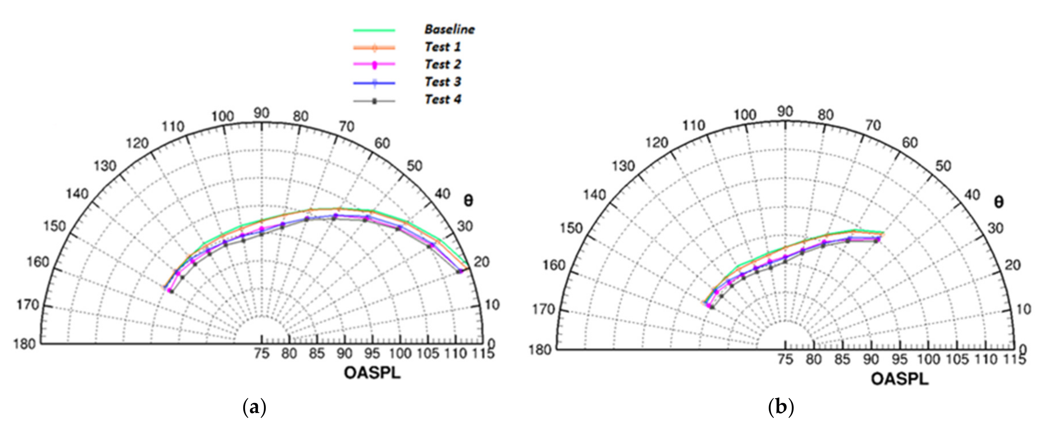
Finally, Figure 19 shows the directivity patterns achieved with the tested fluidic injection system. It has been observed that the fluid injection technique produces a reduction of the OASPL compared to the baseline condition in all the four tests analyzed. In particular, in the fourth test condition the maximum reduction of the OASPL, of about 3.5 dB, is achieved at each directivity angle.
The experimental tests, carried out in this section, show that the fluid injection technique allows to reduce the jet-noise.
4. Conclusions
This paper illustrates the use of a computational aeroacoustics approach, named SNGR (Stochastic Noise Generation and Radiation), based on CFD RANS solutions, and aimed at jet-noise prediction and reduction.
The SNGR method, used in the present work, reconstructs the turbulent velocity fluctuations and calculates the source terms of Vortex Sound acoustic analogy equation, by using Green’s free-field function.
In the first part of this work, the Andersson’s test case has been reproduced to validate the coupled RANS–SNGR approach for its subsequent use as a design tool. The numerical results of aerodynamic and acoustic fields, obtained with the coupled RANS–SNGR approach, have been successfully assessed and validated against both experimental data and results of Large–Eddy Simulations (LES).
In the second part, a technique based on injecting small jets of secondary air, drained from the turbine, into the main jet flow is proposed and assessed. The fluid injection technique, unlike fixed and passive reduction systems such as mechanical chevrons, can be used in all cases that present a real need for noise reduction, such as takeoff and landing phases when the most intense phenomenon of jet noise takes place.
Four tests were carried out, involving gas bleed from the turbine and subsequent injections into the main flow of exhaust gas with the aim of aiding a greater mixing and breaking the large turbulent structures. The four tests have analyzed the influence on the noise reduction of several parameters, such as drained mass flow rate, the area of the injection section and the slope angle of the secondary jets at the same drained pressure and temperature. The best result was obtained in the 4th test, characterized by = 5% , 𝑃𝑠𝑝𝑖𝑙𝑙 = 250,000 Pa, 𝑇𝑠𝑝𝑖𝑙𝑙 = 367.2 K, 𝐴𝑖𝑛𝑗 = 80 mm2, γ = 80° and 𝑢𝑖𝑛𝑗 = 720 m/s, where the maximum noise reduction was achieved, by approximately 3.5 dB compared to Andersson’s baseline case without injection.
Therefore, such tests have confirmed that the fluid injection technique allows an effective jet noise reduction. Moreover, like pointed out by the parametric study discussed in the previous section, the fluid injection technique can be designed as an active and adaptive system, after a proper optimization of several parameters, like the drained mass flow rate, the related pressure and temperature, the injection section area and jet angle, depending on the flight and engine operative conditions.
This kind of fluid injection technique will be controlled by an electronic control unit, in order to produce air outflows from the turbine, and then injections within the gas flow, only when needed. The electronic control of the fluid injection also should allow to regulate at any time the bled mass flow and the temperature and outlet pressure values, in order to optimize the noise reduction in accordance with the operating conditions. Finally, the efficacy of this technique can be further enhanced by azimuth control of the injections, which varies with the operating conditions.
Acknowledgments
This work was conducted as part of the framework of DANTE project (Development of Aero-vibroacoustics Numerical and Technical Expertise), funded under the Italian Aerospace Research Program (PRORA).
Author Contributions
Mattia Barbarino programmed and set the SNGR code for the numerical prediction of jet-noise and designed the noise reduction concept. Mario Ilsami performed the CFD simulations of the aerodynamic field and carried out the comparison with experimental data and LES results. Raffaele Tuccillo determined the features of the jet-noise reduction system and organized the numerical test campaign. Luigi Federico provided hints on SNGR applications and on techniques of noise reduction.
Conflicts of Interest
The authors declare no conflict of interest.
Nomenclature
| A | numerical constant |
| Ainj | injection section area |
| stochastic model parameters | |
| constant pressure and costant volume specific heat | |
| D | nozzle diameter |
| E | monodimensional turbulent kinetic energy spectrum |
| G | Green function |
| K | turbulent kinetic energy |
| k | acoustic wave number |
| k | turbulent wave vector |
| wave number of maximum E | |
| Kolmogorov wave number | |
| turbulence integral length scale | |
| M | Mach number |
| convective Mach number | |
| mass flow rate | |
| number of Fourier modes | |
| number of grid points per Fourier component | |
| p | acoustic pressure |
| probability density function | |
| jet pressure and temperature at the nozzle inlet section | |
| jet pressure and temperature at the nozzle outlet section | |
| ambient pressure and temperature | |
| pressure and temperature of the drained mass flow rate | |
| R | microphone radial distance |
| jet Reynolds number based on nozzle diameter | |
| St | Strouhal number |
| t | time |
| U | mean-flow velocity |
| jet centerline velocity and Mach number at nozzle outlet section | |
| fluctuating turbulent velocity and vorticity | |
| injection velocity | |
| magnitude, phase and direction of nth Fourier component of u′ | |
| turbulent wave vector random angles | |
| injection angle | |
| maximum distance between node i and its neighboring nodes j | |
| cubic cells dimension of 3D domain | |
| turbulent velocity difference | |
| turbulent dissipation rate | |
| kinematical viscosity | |
| vortex convection velocity ratio | |
| radian frequency or specific turbulent dissipation rate | |
| t | time |
| mean-flow velocity | |
| jet centerline velocity and Mach number at nozzle outlet section |
References
- Colonius, T.; Lele, S.K.; Moin, P. Sound generation in a mixing layer. J. Fluid Mech. 1997, 330, 375–409. [Google Scholar]
- Colonius, T.; Mohseni, K.; Freund, J.B.; Lele, S.K.; Moin, P. Evaluation of noise radiation mechanisms in a turbulent jet. In Proceedings of the Summer Program of Center for Turbulence Research, Stanford, CA, USA, 2 June 1998; pp. 159–167. [Google Scholar]
- Freund, J. Noise Sources in a Low-Reynolds-number Turbulent Jet at Mach 0.9. J. Fluid Mech. 2011, 438, 277–305. [Google Scholar] [CrossRef]
- Mitchell, B.; Lele, S.; Moin, P. Direct Computation of the Sound Generated by Vortex Pairing in an Axisymmetric Jet. J. Fluid Mech. 1999, 383, 113–142. [Google Scholar] [CrossRef]
- Bogey, C.; Bailly, C.; Juvè, D. Computation of the Sound Radiated by a 3-D Jet Using Large Eddy Simulation. In Proceedings of the 6th AIAA/CEAS Aeroacoustics Conference, Lahaina, HI, USA, 12–14 June 2000. [Google Scholar]
- Mankbadi, R.; Shih, S.; Hixon, R.; Povinelli, L. Direct Computation of Jet Noise Produced by Large-Scale Axisymmetric Structures. J. Propuls. Power 2000, 16, 207–215. [Google Scholar] [CrossRef]
- Andersson, N.; Eriksson, L.E.; Davidson, L. A Study of Mach 0.75 Jets and Their Radiated Sound Using Large-Eddy Simulation. In Proceedings of the 10th AIAA/CEAS Aeroacoustics Conference, Manchester, UK, 10–12 May 2004. [Google Scholar]
- Kraichnan, R.H. Diffusion by a Random Velocity Field. Phys. Fluids 1970, 13, 22–31. [Google Scholar] [CrossRef]
- Fung, J.C.H.; Hunt, J.C.R.; Malik, N.A.; Perkins, R.J. Kinematic Simulation of Homogeneous Turbulence by Unsteady Random Fourier Modes. J. Fluid Mech. 1992, 236, 281–318. [Google Scholar] [CrossRef]
- Béchara, W.; Bailly, C.; Lafon, P.; Candel, S. Stochastic Approach to Noise Modeling for Free Turbulent Flows. AIAA J. 1994, 32, 455–464. [Google Scholar] [CrossRef]
- Bailly, C.; Juvé, D. A Stochastic Approach to Compute Subsonic Noise Using Linearized Euler’s Equations. In Proceedings of the 5th AIAA/CEAS Aeroacoustics Conference, Seattle, WA, USA, 8–9 November 1999. [Google Scholar]
- Billson, M.; Eriksson, L.; Davidson, L. Jet Noise Modeling Using Synthetic Anisotropic Turbulence. In Proceedings of the 10th AIAA/CEAS Aeroacoustics Conference, Manchester, UK, 10–12 May 2004. [Google Scholar]
- Casalino, D.; Barbarino, M. Stochastic Method for Airfoil Self-Noise Computation in Frequency-Domain. AIAA J. 2011, 49, 2453–2469. [Google Scholar] [CrossRef]
- Di Francescantonio, P. Side Mirror Noise with Adaptive Spectral Reconstruction. In Proceedings of the SAE 2015 Noise and Vibration Conference and Exhibition, Grand Rapids, MI, USA, 22–25 June 2015. [Google Scholar]
- Lighthill, M.J. Jet Noise. AIAA J. 1963, 1, 1507–1517. [Google Scholar] [CrossRef]
- Bridges, J.; Brown, C.A. Parametric Testing of Chevrons on Single Flow Hot Jets: NASA TM 2004–213107. In Proceedings of the 10th AIAA/CEAS Aeroacoustics Conference, Manchester, UK, 10–12 May 2004. [Google Scholar]
- Engblom, W.A.; Kharavan, A.; Bridges, J. Numerical Prediction of Chevron Nozzle Noise Reduction Using WIND-MGBK Methodology. In Proceedings of the 10th AIAA/CEAS Aeroacoustics Conference, Manchester, UK, 10–12 May 2004. [Google Scholar]
- Birch, S.F.; Lyubimov, D.A.; Maslov, V.P.; Secundov, A.N. Noise Prediction for Chevron Nozzle Flows. In Proceedings of the 12nd AIAA/CEAS Aeroacoustics Conference, Cambridge, MA, USA, 8–10 May 2006. [Google Scholar]
- Massey, S.J.; Elmiligui, A.A.; Hunter, C.A.; Thomas, R.H.; Pao, S.P.; Mengle, V.G. Computational Analysis of a Chevron Nozzle Uniquely Tailored for Propulsion Airframe Aeroacoustics. In Proceedings of the 12nd AIAA/CEAS Aeroacoustics Conference, Cambridge, MA, USA, 8–10 May 2006. [Google Scholar]
- Shur, M.L.; Spalart, P.R.; Strelets, M.K. Noise Prediction for Increasingly Complex Jets, Part II: Applications. Int. J. Aeroacoustics 2005, 4, 247–266. [Google Scholar] [CrossRef]
- Shur, M.L.; Spalart, P.R.; Strelets, M.K.; Garbaruk, A.V. Further Steps in LES-Based Noise Prediction for Complex Jets. In Proceedings of the 44th AIAA Aerospace Sciences Meeting and Exhibit, Reno, NV, USA, 9–12 January 2006. [Google Scholar]
- Henderson, B.S.; Kinzie, K.W.; Whitmire, J.; Abeysinghe, A. The impact of fluidic chevrons on jet noise. In Proceedings of the 11th AIAA/CEAS Aeroacoustics Conference, Monterey, CA, USA, 23–25 May 2005. [Google Scholar]
- Kinzie, K.W.; Henderson, B.S.; Whitmire, J.; Abeysinghe, A. Fluidic chevrons for jet noise reduction. In Proceedings of the 2004 International Symposium on Active Control of Sound and Vibration (ACTIVE 2004), Williamsburg, VA, USA, 20–22 September 2004. [Google Scholar]
- Henderson, B.S.; Kinzie, K.W.; Whitmire, J.; Abeysinghe, A. Aeroacoustic Improvements to Fluidic Chevron Nozzles. In Proceedings of the 12th AIAA/CEAS Aeroacoustics Conference, Cambridge, MA, USA, 8–10 May 2006. [Google Scholar]
Figure 1.
Representation of the wave vector and velocity direction vector and definition of the stochastic angles (Adapted from [13]).
Figure 1.
Representation of the wave vector and velocity direction vector and definition of the stochastic angles (Adapted from [13]).

Figure 2.
Two-point space correlation of a jet plume. (a) First approach based on blobs structure; (b) Second approach based on an adaptive Cartesian mesh.
Figure 2.
Two-point space correlation of a jet plume. (a) First approach based on blobs structure; (b) Second approach based on an adaptive Cartesian mesh.

Figure 3.
Computational domain (Adapted from Andersson [7]).
Figure 3.
Computational domain (Adapted from Andersson [7]).

Figure 4.
(a) Mesh used for the Reynolds Averaged Navier Stokes (RANS) jet flow simulation; (b) Contour plots of the RANS solution. Mean velocity on the top and turbulent kinetic energy on the bottom.
Figure 4.
(a) Mesh used for the Reynolds Averaged Navier Stokes (RANS) jet flow simulation; (b) Contour plots of the RANS solution. Mean velocity on the top and turbulent kinetic energy on the bottom.

Figure 5.
The vertical dashed lines indicate lines along which profiles of time-averaged quantities were extracted (Adapted from Andersson [7]).
Figure 5.
The vertical dashed lines indicate lines along which profiles of time-averaged quantities were extracted (Adapted from Andersson [7]).

Figure 6.
(a) Centerline profile of the axial velocity; (b) Axial profiles of turbulence intensity. (Dotted black lines: experimental results; continuous red line: K-ε model; dashed green line: K-ω SST model; dotted-dashed blue line: LES).
Figure 6.
(a) Centerline profile of the axial velocity; (b) Axial profiles of turbulence intensity. (Dotted black lines: experimental results; continuous red line: K-ε model; dashed green line: K-ω SST model; dotted-dashed blue line: LES).

Figure 7.
(a) Radial profiles of axial velocity; (b) Radial profiles of uv correlation. The profiles have been staggered according to their axial location. (Dotted black lines: experimental results; continuous red line: K-ε model; dashed green line: K-ω SST model; dotted-dashed blue line: LES).
Figure 7.
(a) Radial profiles of axial velocity; (b) Radial profiles of uv correlation. The profiles have been staggered according to their axial location. (Dotted black lines: experimental results; continuous red line: K-ε model; dashed green line: K-ω SST model; dotted-dashed blue line: LES).

Figure 8.
(a) 3D acoustic domain; (b) 3D contour plot of turbulent kinetic energy.

Figure 9.
Position of the microphones (Adapted from Andersson [7]).
Figure 9.
Position of the microphones (Adapted from Andersson [7]).

Figure 10.
(a) Power spectra of far-field pressure signal for a few observer locations on the inner arc, . The Power Spectral Density (PSD) spectra have been staggered by multiplying the amplitude by a factor , where and being the angle from the jet axis; (b) Overall Sound Pressure Level Directivity.

Figure 11.
(a) Power spectra of far-field pressure signal for a few observer locations on the outer arc, . The PSD spectra have been staggered by multiplying the amplitude by a factor , where and being the angle from the jet axis; (b) Overall Sound Pressure Level Directivity.
Figure 11.
(a) Power spectra of far-field pressure signal for a few observer locations on the outer arc, . The PSD spectra have been staggered by multiplying the amplitude by a factor , where and being the angle from the jet axis; (b) Overall Sound Pressure Level Directivity.

Figure 12.
Sound radiation from the jet. Real part of the acoustic pressure [Pa] at 700 Hz.

Figure 13.
Sketch of the active Fluidic Injection System.

Figure 14.
Sketch of the low frequency turbulence region.

Figure 15.
Sketch of the exhaust plumes emitted from a jet engine without (on the top) and with fluid injection (on the bottom).
Figure 15.
Sketch of the exhaust plumes emitted from a jet engine without (on the top) and with fluid injection (on the bottom).

Figure 16.
Turbulent kinetic energy levels [m2/s2] for the injection patterns tested.

Figure 17.
Comparison between the different injection patterns in terms of velocity and turbulence intensity. (a) Centerline profile of the axial velocity; (b) Axial profiles of turbulence intensity.
Figure 17.
Comparison between the different injection patterns in terms of velocity and turbulence intensity. (a) Centerline profile of the axial velocity; (b) Axial profiles of turbulence intensity.

Figure 18.
Turbulent velocity difference, Δ𝑢𝑡𝑢𝑟𝑏 [m/s] between the baseline case and the 4th test in the whole domain of interest.
Figure 18.
Turbulent velocity difference, Δ𝑢𝑡𝑢𝑟𝑏 [m/s] between the baseline case and the 4th test in the whole domain of interest.

Figure 19.
(a) Overall Sound Pressure Level Directivity on the inner arc; (b) Overall Sound Pressure Level Directivity on the outer arc.
Figure 19.
(a) Overall Sound Pressure Level Directivity on the inner arc; (b) Overall Sound Pressure Level Directivity on the outer arc.


Table 1.
Test matrix for the injection system design.
| TEST | Injection Mass Flow Rate/Nozzle Mass Flow Rate | Injection Section Area/Nozzle Outlet Area | Injection Direction [deg] | Injection Velocity [m/s] |
|---|---|---|---|---|
| 1 | 13.0% | 10.2% | 45 | 350 |
| 2 | 13.0% | 10.2% | 60 | 450 |
| 3 | 13.0% | 10.2% | 80 | 690 |
| 4 | 6.5% | 4.08% | 80 | 720 |
© 2017 by the authors. Licensee MDPI, Basel, Switzerland. This article is an open access article distributed under the terms and conditions of the Creative Commons Attribution (CC BY) license (http://creativecommons.org/licenses/by/4.0/).
Share and Cite
MDPI and ACS Style
Barbarino, M.; Ilsami, M.; Tuccillo, R.; Federico, L. Combined CFD-Stochastic Analysis of an Active Fluidic Injection System for Jet Noise Reduction. Appl. Sci. 2017, 7, 623. https://0-doi-org.brum.beds.ac.uk/10.3390/app7060623
AMA Style
Barbarino M, Ilsami M, Tuccillo R, Federico L. Combined CFD-Stochastic Analysis of an Active Fluidic Injection System for Jet Noise Reduction. Applied Sciences. 2017; 7(6):623. https://0-doi-org.brum.beds.ac.uk/10.3390/app7060623
Chicago/Turabian StyleBarbarino, Mattia, Mario Ilsami, Raffaele Tuccillo, and Luigi Federico. 2017. "Combined CFD-Stochastic Analysis of an Active Fluidic Injection System for Jet Noise Reduction" Applied Sciences 7, no. 6: 623. https://0-doi-org.brum.beds.ac.uk/10.3390/app7060623
Note that from the first issue of 2016, this journal uses article numbers instead of page numbers. See further details here.