
Random Forest Prediction of IPO Underpricing


Department of Computer Science and Engineering, Universidad Carlos III de Madrid, 28903 Madrid, Spain
*
Author to whom correspondence should be addressed.
Appl. Sci. 2017, 7(6), 636; https://0-doi-org.brum.beds.ac.uk/10.3390/app7060636
Submission received: 2 May 2017
/
Revised: 12 June 2017
/
Accepted: 15 June 2017
/
Published: 20 June 2017
Abstract
:The prediction of initial returns on initial public offerings (IPOs) is a complex matter. The independent variables identified in the literature mix strong and weak predictors, their explanatory power is limited, and samples include a sizable number of outliers. In this context, we suggest that random forests are a potentially powerful tool. In this paper, we benchmark this algorithm against a set of eight classic machine learning algorithms. The results of this comparison show that random forests outperform the alternatives in terms of mean and median predictive accuracy. The technique also provided the second smallest error variance among the stochastic algorithms. The experimental work also supports the potential of random forests for two practical applications: IPO pricing and IPO trading.

1. Introduction
The magnitude of initial returns in initial public offerings (IPOs) has been puzzling both researchers and practitioners for decades. The difference between the offering price and the first closing price regularly results in sizeable gains or losses. Among these, there is a bias in the distribution of initial returns that is positive and heavily skewed to the right. For this reason, first-day initial returns are often referred to in the literature as IPO underpricing.
During the Internet bubble of the late 1990s, when the market was very hot, a substantial portion of the companies taken public in the USA more than doubled their offering price in the first day and the phenomenon often resulted in headlines in the news. Ritter and Welch [1] researched the phenomenon, and reported that the average initial return on a sample of 6249 companies taken public in the USA between 1980 and 2001 was 18.8%. More recently, the number of IPOs has dramatically gone down, and so has the average initial return. Having said that, in 2014 Castlight, San Francisco, CA, USA, a health care software company, soared 149% during its first trading day. Another recent example, though more limited, would be Alibaba Group, Hangzhou, China, the e-commerce giant. This corporation showed a 38% increase from its initial public offering price on the day it went public.
The academic literature has been tracking first-day trading returns in initial public offerings (IPOs) for a long time. Over time, researchers have postulated a large number of explanatory theories, and it is still a very active field of investigation. The vast majority of the empirical analyses carried out to explain and predict underpricing relying on variables related to the structure of the offerings are based on linear models. There have been, however, a number of efforts trying to predict first-day returns using computational intelligence.
Among the latter, we should mention the work of Jain and Nag [2]. These authors try to predict the post-issue market price using artificial neural networks. More recently, Reber et al. [3], Meng [4], Chen [5], and Esfahanipour et al. [6] followed suit with the same technique. This line was complemented by Quintana et al. [7] and Luque et al. [8], who explored the problem using evolutionary algorithms. Others, such as Chou et al. [9], used a combination of both of them.
In this paper, we suggest that there is an instrument that has not been tested in the domain yet, that has the potential to be extremely valuable. In a field where the presence of outliers and the problem of overfitting severely affects the performance of predictive algorithms, random forests [9], are likely to bring a great deal to the table. For this reason, we intend to benchmark the random forests on a sample from the USA financial markets against a number of classic machine learning alternatives that represent different algorithm categories.
The rest of the paper will be structured as follows: in Section 2, we provide a brief introduction to random forests and introduce both the explanatory variables and the sample that will be used in the analysis; Section 3 will be used to report the experimental results; that will be followed by a discussion in Section 4; and, finally, Section 5 will cover the summary and conclusions.
2. Materials and Methods
Random forests [10] are ensemble learning methods that combine trees of predictors. This approach, which is usually treated as a supervised method, creates sets of decision trees that vote for the most popular class for vectors according to a number of features.
The trees in a forest are created according to a procedure that is similar to classification and regression trees. The previous element is combined with randomized node optimization and bagging. According to Breiman, the author who introduced the technique, the process follows three key ideas:
- Each tree is grown based on a unique training set that is generated by a random sampling with replacement from the original dataset. The size of this new sample mirrors the size of the initial one.
- For every node, a subset of the original input variables is selected at random, and the best-performing split on these is used to split the node. The size of the mentioned subset is kept constant during the forest growing.
- Trees are grown to the largest extent possible while complying with a minimum number of training patterns at a terminal node constraint, leaf size, and there is no pruning.
The resulting set can then be used to make predictions using a voting mechanism. The process simply entails obtaining individual class predictions for unseen samples from all the components of the forest, and assigning the data pattern to the majority vote.
This technique is applicable to both classification and regression tasks. IPO underpricing prediction falls in the latter category. In this case, tree predictors take on numerical values instead of class labels, and the predictor is formed by taking the average prediction from the tree set.
Random forests show a major strength vs. other tree-based techniques, such as bagging, that is likely to be useful in the IPO domain. Specifically, the ability to combine strong and weak variables to generate models where the former do not dominate tree generation is a key property. The reason is that it affects the correlation among tree output and, therefore, the generalization error of the model. Krauss et al. [11] show that random forests are the dominant single method for deriving trading decisions on the Standard and Poor′s (S&P) 500 stock universe vis-à-vis deep neural networks and gradient-boosted trees. Other general properties that are relevant in the IPO underpricing prediction domain are its relative robustness with regard to outliers in training data and the fact that it does not overfit.
The use of random forests to tackle financial problems is not new. Recent papers illustrate potential application areas, such as trading [12], bankruptcy prediction [13,14], or credit rating prediction [15], but, as we mentioned in the introduction, despite the desirable traits, its suitability for IPO underpricing prediction is still to be studied.
2.1. Variables
The starting point to study the phenomenon of IPO underpricing, the most prevalent target variable on IPO research, is providing a formal definition. IPO underpricing, Ri, is defined in this paper as the percentage difference between the offer price and the closing price on the first trading day, adjusted for the market return:
where Poi represents the offering price for stock i; Pci is the closing price for stock i; Moi is the opening for the broad market index of the market where stock i was taken public for the day before the IPO and Mci is the closing for market index on the day of the IPO. For the purposes of this study, the relevant indices are the S&P 500, AMEX Composite Index, and NASDAQ Composite Index.
As we have already discussed, the body of research on IPO initial returns is vast. The number of explanations and variables that have been postulated to explain the phenomenon is very wide. However, there is a set of independent variables concerning the structure of the offerings that show up in the literature very often. Among them, we relied on six that we will succinctly describe: width of the price range; offer price; price adjustment; relation to the tech sector; offering size; and retained stock.
- Width of price range (RANGE): the width of the non-binding reference price range offered to potential investors during the roadshow has been traditionally considered to have a signaling effect. Wider ranges show uncertainty regarding the valuation of the company and, therefore, tend to be associated with riskier investments. Following [16,17], this indicator will be defined as the difference between the maximum and minimum price, divided by the minimum.
- Price adjustment (P_ADJ): many studies such as Hanley [16], Benveniste and Spindt [20], or Ljungqvist and Wilhelm [21] show that relation between the initial tentative price range and the final offer price might be interpreted as a signal by investors. These authors suggest that this effect is likely to be captured the expression that follows:where Pf is the offer price and Pe, the expected price, is the price at the middle of the non-binding reference range.
- Technology (TECH): companies whose industrial activities are related to the technology sector tend to show higher initial returns. This is usually controlled in the models by means of a dummy variable that equals one for tech companies and zero otherwise [22,23,24]. Our labeling criterion will be based on the definition used by IPO Monitor. This company classifies IPOs according the US Standard Industry Codes and activities reported by the companies in their filings. Hence, we will consider IPOs to be “tech-related” if IPO Monitor considers them so in their reports.
- Retained stock (RETAINED): the amount of capital retained by initial investors has been traditionally interpreted as a signal of the quality of the stock, as it would reveal the confidence of insiders in the future of the company [21,27]. Since we lack the breakdown of primary and secondary shares, this variable will be proxied by the ratio of the amount of shares sold at the IPO divided by the post-offering number of shares minus the shares sold at the IPO.
2.2. Data
The experimental work is based on a sample of 866 companies taken public between January 1999 and May 2010 in three US stock markets, AMEX, NASDAQ, and NYSE (the New York Stock Exchange). As it is customary in IPO research, it excludes closed-end funds; American Depositary Receipts; Real estate investment trusts (REITs), and unit offerings. The primary source of data was the commercial provider IPO Monitor. Missing information was completed with data from a second data vendor, Hoovers. Finally, index information was retrieved from DataStream (S&P 500) and NASD (NASDAQ and AMEX composites).
Table 1 reports the main descriptive statistics (mean, median, standard deviation, minimum, and maximum) for the sample.
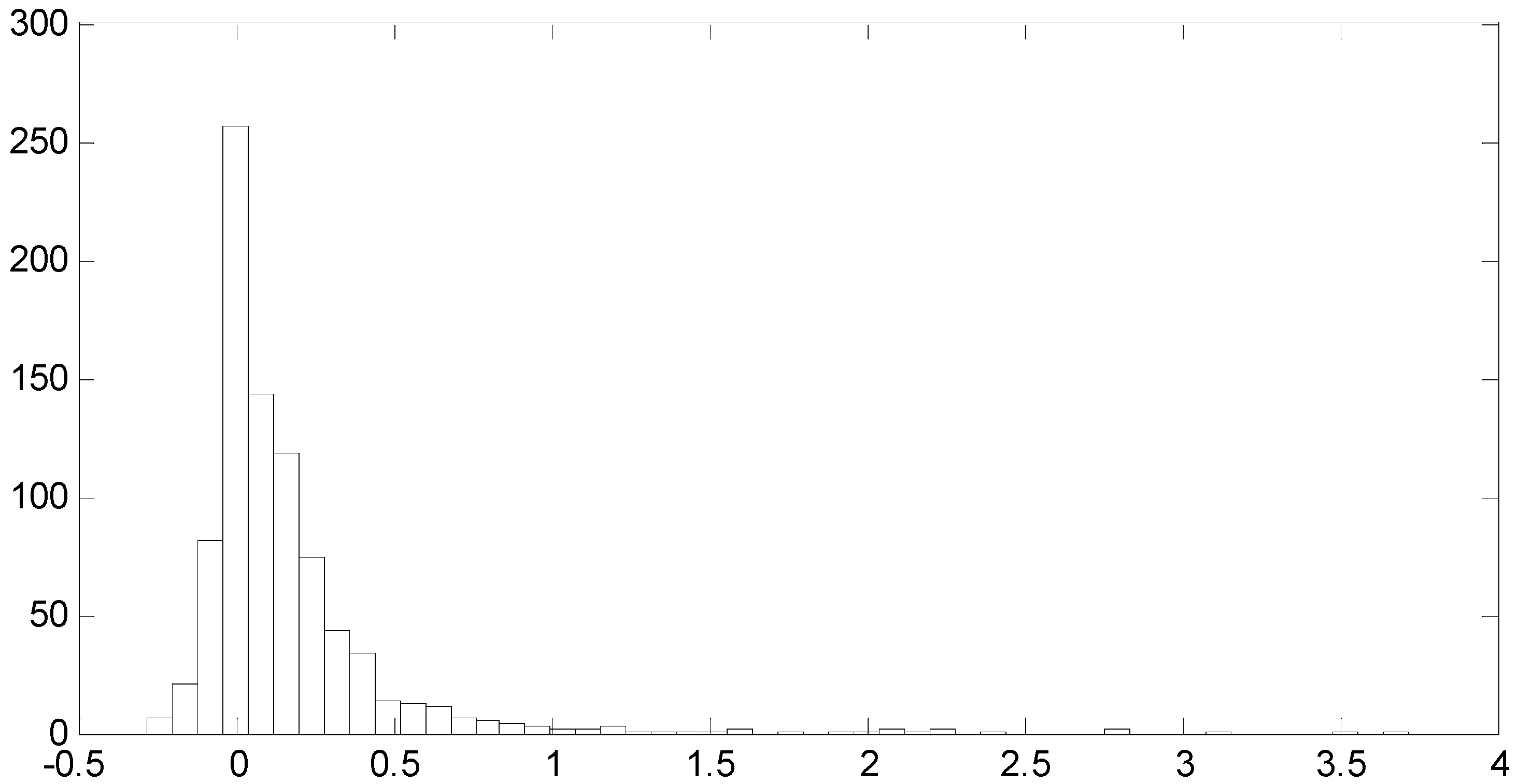
Figure 1 shows the return distribution. As we can see, it shows a positive mean return, high kurtosis, and the classic right-skewness corresponding to several hot IPOs with extremely high initial returns (in this case, the most extreme case almost got to quadruple the offering price with a 372% price increase). The mentioned basic characteristics are consistent with the structure of the sample used in previous studies, such as [1,7,18,19,21], among many others.
2.3. Methodology
The experimental analysis started with an initial exploratory analysis followed by the main experiments intended to test the predictive accuracy of random forests.
As a first step, we selected the appropriate parameters for the algorithm: leaf size and number of grown trees. This initial analysis was made on a subset of 256 patterns, approximately 30% of the data. The selection of the set of IPOs included in this subsample was random, and these patterns were excluded from the test sample used in the main experiments, that comprised of the remaining 610 IPOs.
We chose one third of the input features for decision splits at random and subsequently tested different combinations of number of trees and leaf sizes ranging from five to 25. As we can see in Figure 2, these parameters have a major impact on the results.
We conducted several experiments and we saw that the progressive addition of trees resulted in patterns of out-of-bag, OOB, prediction errors such as the one represented in the figure. There, we can observe that the root mean square error (RMSE) on the cases left out of the bootstrap sample used in the construction of the trees tends to stabilize with 40–50 elements. For this reason, we decided to set the number of grown trees at 45. We also fixed at five the minimum number of training patterns per terminal node. It is worth noting that this figure matches the standard rule-of-thumb used in regression problems.
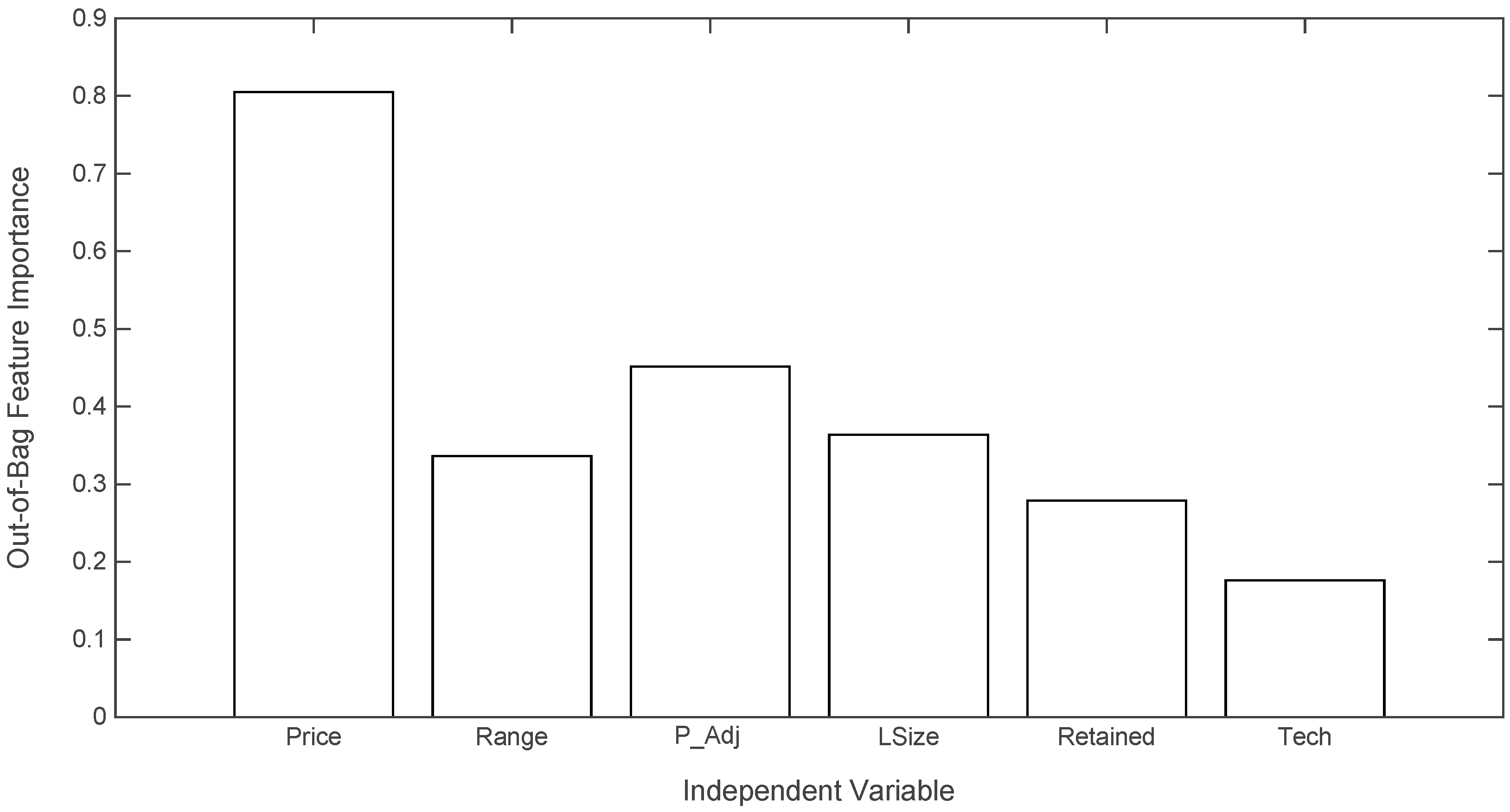
As part of this preliminary analysis, we also studied the relative explanatory power of the independent variables. We assessed the out-of-bag feature importance by the mean decrease in accuracy [28]. This indicator, also known as permutation importance, evaluates the contribution of independent variables by removing the association between predictor variables and the target. The rationale is that a random permutation of the values of the feature mimics the absence of the variable from the model, and the resulting increase of error can be used as an importance measure. More formally, the procedure carried out was the following: for any variable, we computed the increase in the prediction error if the values of that variable were permuted across the out-of-bag observations. Once we obtained the measure for every tree, we averaged it over the entire ensemble and divided it by the standard deviation for the entire ensemble. The last step was carried out to standardize the raw variable importance score. The results of this process are reported in Figure 3. There, we can see how the offering price is the most relevant variable in the set. The second, most explanatory variable is the price adjustment made by the seller once he has received the initial show of interest during the road-show, closely followed by the offering size. Among the rest, the dummy variable signaling whether the company is part of the tech sector or not, seems to be the least important one. The prevalence of price vs. the rest clearly illustrates the need for a technique that efficiently combines strong and weak variables that we mentioned in the introduction to random forests.
2.4. Benchmarks
We intend to benchmark random forests against a set of machine learning alternatives. For implementation purposes, we will rely on a very popular collection of machine learning algorithms called WEKA (Waikato Environment for Knowledge Analysis) [29]. The algorithms we will use as benchmarks are: instance-based learning algorithms (IBK); least median of squares regression (LMSReg); locally-weighted learning (LWL); M5 model trees (M5P); M5 model rules (M5Rules); multilayer perceptron (MLP); radial basis function networks (RBFN); and support vector machines trained with sequential minimal optimization (SMO-Reg). This selection of algorithms includes different categories, such as alternatives based on functions, nearest neighbors, rules, and decision trees.
- IBK [30]: an implementation of a K-nearest neighbor classifier.
- LMSReg [31]: a robust linear regression approach that filters out outliers in order to enhance accuracy.
- LWL [32]: a local instance-based learning algorithm that builds classifiers based on weighted instances.
- M5P [33]: a numerical classifier that combines standard decision trees with linear regressions to predict continuous variables.
- M5Rules [34]: the algorithm generates decision lists for regression problems using divide-and-conquer. It builds regression trees using M5 in every iteration, and then it turns the best leaves into rules.
- MLP [35]: a standard feed-forward artificial neural network that simulates the biological process of learning through weight adjusting. The algorithm used to train the networks will be back-propagation.
- RBFN [36]: a type of artificial neural network that uses a combination radial basis functions to approximate the structure of the input space.
- SMO-Reg [37]: a support vector machine trained with the sequential minimal optimization algorithm.
All these are described in more detail in Appendix A.
Table 2 summarizes the parameters used to run these algorithms. The selection of the specific values was made according to the performance of the algorithms in an exploratory analysis. Different configurations were tested on the same portion of the sample used to parameterize the random forests, and the final choice was made according to predictive accuracy in terms of RMSE using a 10-fold cross validation. A summary of configurations and results is reported in Appendix B. The results for stochastic algorithms average the outcome of three different experiments.
The models will be assessed by their predictive accuracy in terms of RMSE on the same dataset. In order to make the results as general as possible, we will perform a 10-fold cross-validation. Given the stochastic nature of most of the algorithms, including random forests, we will run the experiments 15 times using different random seeds and compare the average results. We will, however, report the main descriptive statistics of these averages to ensure that the image is complete.
3. Results
In this section we report the results of the experimental analysis performed to test the suitability of the random forest algorithm for the IPO underpricing prediction domain.
The main experimental results are reported in Table 3. There, we provide the main descriptive statistics for the RMSE obtained in the 15 repetitions of the 10-fold cross-validation. For stochastic algorithms we report the average, median, variance, maximum, and minimum. The exception to this is SMO-Reg. Even though it has a stochastic component and we used different seeds, the 15 experiments converged to the exact same solution.
The statistical significance of the differences reported in Table 3 was tested formally. Given the distribution of the prediction errors, we relied on the Mann–Whitney test [38]. The results of this analysis are reported in Table 4. There, we represent the fact that the algorithm in the row has median prediction error that is significantly larger than the one in the column at 1% by “++”. In case a similar difference in the opposite direction is found, the symbol used is “--”. If the disparity is such that the first one is significantly smaller at 5%, we use “-”. Finally, if the possibility of equal predictive accuracy cannot be discarded at 5%, we report “=”.
Following [3], we complement the analysis based on predictive performance illustrating the potential economic benefits of using these techniques to price IPOs. In Table 5 we compare the actual observed underpricing with the initial returns resulting should we use forecasts of the models as the offering price. For each of the models, we provide the average value of the statistics on the 610-pattern test set over 15 experiments. That is, we report the average mean underpricing, average median underpricing, and the average of the standard deviations. All of the differences between the median mean observed underpricing and model-based ones were significant at 1%.
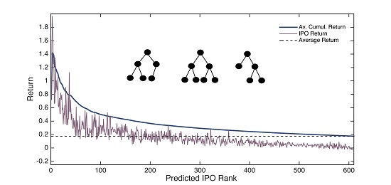
Random forests can also be used in this context as an investment tool. A potential trading strategy would be investing in IPOs with the highest initial return potential according to the models. Even though the predictions for initial returns might not be completely accurate, the distribution of forecasts could provide very valuable insights. This is evidenced by Figure 4. There, we report the returns obtained investing in IPOs prioritized according to the forecasts of the models. The 610 IPOs that compose the test set were ranked by predicted return. Given that we repeated the experiments 15 times, we obtained as many ranks. The IPO Return series shows the average of the actual returns that correspond to the 15 IPOs that have the same rank. The series labeled Av. Cumul. Return, represents the cumulative average of actual returns. For example, the return for IPO 100 was obtained by computing the actual mean underpricing of the 100 companies with the highest predicted initial return. This process was repeated for the 15 experiments, and we report the observed mean cumulative average return. Finally, we include the actual average underpricing to represent the naïve strategy of investing in all IPOs.
4. Discussion
As we can in Table 3, random forests provide the best results, followed by IBK. In addition to the relatively low mean and median RMSE, we should highlight the fact that the approach seems to be the second-most reliable one among those with a stochastic component. The range of variation for the prediction error is narrow and its variance is relatively low. It was only beaten by SMO-Reg. This algorithm offered an intermediate performance in terms forecasting ability, but converged to the same solution across the 15 experiments.
On the opposite side of the spectrum, LWL and MLP offered the worst results. Even though multi-layer perceptrons have been successfully used in many regression tasks, their sensitivity to the presence of outliers drags its performance in this domain. Conversely, random forests handle this difficulty with much more efficacy. MLP showed the highest dispersion of results, including the worst prediction error in one of the executions.
If we consider the potential economic implications of the potential of using random forests in this domain, the results lay down two interesting applications: IPO pricing, and investing. On the first front, random forests offered the lowest average difference between the actual closing price and the predicted one. This reduced model-based underpricing, where offer price is replaced with the output of the model, came together with the smallest average standard deviation. The implication is that the use of this algorithm to support the pricing decision is likely to have the potential to reduce the amount of money left of the table.
On the second front, Figure 4 makes it apparent that there could be room for profitable trading based on the output of the models. Even though we cannot claim that random forests make perfect initial return predictions based on the variables discussed, they show good capabilities ranking them. IPOs that are predicted to offer the highest initial returns suffer significantly higher underpricing than the expected bottom performers.
As we can see by the spikes of the IPO Return series, the models do not have the ability to rank perfectly. The highest initial return does not correspond to the first element of the series, and it is far from smooth. In addition to that, the 15 experiments do not result in the same rank (that is, the reason why the maximum value of the series is lower than the highest initial return). Having said that, as the highest values clearly tend to be at the beginning of the series and the lowest at the end, if we invested if the n most promising ones we would be very likely to gain excess returns. That would happen as long as the average return, shown in the Average Cumulative Return series, is higher than the IPO market return, Average Return, and the difference is enough to cover the transaction costs.
A basic trading strategy would require establishing buy thresholds based on the distribution of underpricing predictions and the ability to invest on all IPOs, which might not always be a possibility. As several theories discussed in [1] suggest, factors such as higher demand for promising IPOs, laddering practices, or book building strategies by underwriters, are likely to result in higher allocation of bottom performers and lower than desired, if any, of the good ones. This means that the naïve strategy might not be as lucrative in practice as it may seem at first sight. There are many other alternatives that are worth exploring, but they are beyond the scope of this paper. However, the results of the experiments leave the room open for additional work on random forests for IPO trading.
We should note that the reported performance gap between random forests and the other algorithms might be understated due the decision to focus the analysis on variables related to structure of the offerings. This technique combines efficiently strong and weak variables, and it has already been proven to deal with large numbers of variables in financial applications [39]. Hence, it is likely to profit very significantly from the inclusion of financial ratios and IPOs market indicators. This is something that should be explored in the future.
The results obtained in the experiments support the idea that random forests are suitable in this domain due to the good match, its mentioned characteristics, and the nature of the technique.
5. Summary and Conclusions
IPO underpricing prediction is a domain with some specific characteristics that make it especially challenging. Among them, we could highlight the fact that the set of descriptive variables identified by academic research is limited in their predictive power and mixes both weak and strong predictors. In addition to this, the presence of outliers, that usually take the form of IPOs with extremely high initial returns, adds noise and complicates the process of training models.
In this paper, we suggest that random forests, a technique that, by design, is less sensitive to distortions introduced by the extreme elements in the training sample, could be very useful to perform the task. In order to do that, we test its predictive performance in terms of root mean squared prediction error on a sample of 866 USA IPOs. The approach relied on six variables identified by literature review that were available in commercial databases.
In order to have a meaningful base of comparison, we benchmark the results against eight popular machine learning algorithms: IBK, least median of squares regression, LWL, multilayer perceptron, M5P, M5Rules, radial basis neural networks, and SMO-Regression. This represents different families of predictive algorithms as those based on functions, nearest neighbors, rules, and decision trees.
The outcome of this comparison shows that random forests outperform the alternatives in terms of mean and median predictive accuracy over the 15 repetitions of the 10-fold cross-validation analysis. The technique also provided the second smallest variance and error range among the stochastic algorithms. As an additional side result, we also confirmed the importance of price over the other five predictive variables.
The experimental work also explores the potential of the technique on two practical fronts: as an IPO pricing support tool, and as the core of IPO trading strategies. The usefulness of random forests for both applications is supported by the results. On the one hand, model-based average underpricing is both the lowest among the benchmarked alternatives, and significantly smaller than the actual observed one. On the other hand, the algorithm shows strong capabilities in terms of ranking IPOs according to their potential initial returns.
The above-mentioned results suggest that IPO research would benefit greatly from a wider use of random forests. Possible future lines of work would include replicating the analysis for samples from other countries and extended sets of independent variables. Another promising line would be exploring in depth the potential or random forests to identify a priori hot IPOs and exploiting this knowledge for investment purposes.
Acknowledgments
The authors acknowledge financial support granted by the Spanish Ministry of Science under grant ENE2014-56126-C2-2-R.
Author Contributions
David Quintana and Pedro Isasi conceived and designed the experiments; David Quintana performed the experiments; David Quintana, Yago Sáez and Pedro Isasi analyzed the data; and David Quintana and Yago Sáez wrote the paper.
Conflicts of Interest
The authors declare no conflict of interest. The founding sponsors had no role in the design of the study; in the collection, analyses, or interpretation of data; in the writing of the manuscript; and in the decision to publish the results.
Appendix A
In this appendix, we provide a very brief description of the algorithms used for benchmarking.
Appendix A.1. Instance-Based Learning Algorithms (IBK)
IBK is an implementation of a standard K-nearest neighbor-algorithm, in this case, for regression. It is instance-based and is one of the simplest machine learning algorithms. Given a point of interest, the approach identifies the k closest training examples in the feature space according to a predefined distance, Euclidean in our experiments. Once this is done, the output for the pattern of interest is the average value of the target variables of the neighbors.
Appendix A.2. Least Median of Squares Regression (LMSReg)
This is a robust linear regression model that filters out outliers to reduce the impact of outliers. Classical least squares regression (OLS) minimizes the sum of square residuals on all data, which makes the model very sensitive to extreme values. This alternative fits models to random subsets of the data and selects the least squared regression with the lowest median squared error. According to the studies of the creators of the technique, the computational cost of this approach is significantly higher than the one required by OLS. However, the models resulting from the mentioned process can resist a contamination in the data of close to 50%.
Appendix A.3. Locally-Weighted Learning (LWL)
Locally-weighted learning covers a number of function approximation methods that, instead of creating a single model based on all data, makes predictions based on models fitted to local subsets based on data around the point of interest. For that purpose, data patterns are associated to weighting factors that represent the contribution of each pattern to the prediction. The contribution of each pattern to the final prediction is based on a weighting function that, most of the time, gives more weight to data patterns that are in the close neighborhood of the query point vs. those that are far. For this matter, the neighborhood can be defined as the whole sample, or be limited to a number of neighbors. Like IBK, one of the interesting features of these algorithms is the fact the processing of the training data is delayed until the system receives queries on specific points of interest.
Appendix A.4. M5 Model Trees (M5P)
M5 is a system that constructs tree-based piecewise linear models that, unlike other tree-based algorithms, has the ability to predict values. The approach, which follows the divide-and-conquer method, differs from similar algorithms such as CART, because instead of having values at the nodes, they contain multivariate linear regressions. M5 divides the input space into smaller areas using training and, subsequently, creates a regression model per area as a leaf of the tree. Some of the interesting features of the algorithm are the fact that it can handle very large of attributes, and the fact the resulting trees are generally smaller than similar approaches, such as regression trees.
Appendix A.5. M5 Model Rules (M5Rules)
This algorithm induces simple decision lists from model trees that are generated using M5. The system builds model trees repeatedly, and every iteration it selects the best rules. Since the algorithm is based the already-mentioned M5, it also relies on the divide-and-conquer principle. The algorithm divides the parameter space into areas and creates a linear regression model for each of them. According to the designers, this approach has the advantage of deriving rule sets that, despite being smaller than those obtained directly from the whole dataset, offer the same performance.
Appendix A.6. Multilayer Perceptron (MLP)
These feed-forward neural network models consist of multiple layers of nodes, also known as neurons, in a directed graph, so that each layer is connected to the next one. All of the nodes, other than those in the input layer, process input signals coming from other neurons, process them with a nonlinear activation function, and propagate the result. The version used in this study consists of three layers—input, hidden, and output—that use a sigmoid transfer function. The strength of the connections, known as weights, and biases are adjusted to fit a dataset through a training process. In this paper, we used retropropagation. Given an input, this gradient descent algorithm compares the output of the network with the desired one, and then propagates the prediction error backwards, starting from the output, adjusting the weights and biases.
Appendix A.7. Radial basis Function Networks (RBFN)
These neural networks use sets of radial basis functions (RBF) as activation functions. The version used in the analysis is structured in three layers. The first one is an input layer, followed by a hidden layer with a non-linear RBF activation function and, finally, a linear output layer. The output of these models is generated by linear radial basis functions of the inputs and neuron parameters. Training usually follows a two-step process that started initializing the center vectors of the RBF functions using the k-means algorithm. That is followed by a second that fits a linear model to the hidden layer’s output with respect the objective function.
Appendix A.8. Support Vector Machines Trained with Sequential Minimal Optimization (SMO-Reg)
Support vector regression models (SVR) are learning machines that implement the structural risk minimization inductive principle. These adapt the original support vector machines that were focused on classification tasks. Unlike traditional regression models, this algorithm does not minimize training errors. Instead, it simultaneously targets the minimization the training error and a regularization term that controls the complexity of the hypothesis space, so as to achieve generalized performance. The models disregard part of the training data, as the cost function ignores the training patterns that are beyond a specified distance to the model prediction. Training these models requires finding solution for convex optimization problems. In this instance, we tackled this latter part using the sequential minimal optimization (SMO) algorithm.
Appendix B
In this appendix, we summarize the results exploratory analysis aimed at parameterizing the benchmark algorithms. Underpricing predictive performance was assessed in terms of RMSE on the 256-pattern training sample. For stochastic algorithms, the reported RMSE is the average of three runs.

Table A1.
Sensitivity of instance-based learning algorithms (IBK) to the number of neighbors.
| Number of Neighbors | RMSE |
|---|---|
| 1 | 0.4793 |
| 2 | 0.4364 |
| 3 | 0.3858 |
| 4 | 0.3832 |
| 5 | 0.3868 |
| 6 | 0.3876 |
Table A2.
Sensitivity of locally-weighted learning (LWL) to the number of neighbors.
| Number of Neighbors | RMSE |
|---|---|
| 1 | 0.4492 |
| 5 | 0.5361 |
| 10 | 0.3678 |
| 15 | 0.5028 |
| 20 | 0.446 |
Table A3.
Sensitivity of M5 model trees (M5P) to the minimum number of instances per leaf.
| Min Instances/Leaf | RMSE |
|---|---|
| 1 | 0.405 |
| 5 | 0.405 |
| 10 | 0.3916 |
| 15 | 0.3894 |
| 20 | 0.3896 |
| 25 | 0.3918 |
Table A4.
Sensitivity of M5 model rules (M5Rules) to the minimum number of instances per leaf.
| Min Instances/Leaf | RMSE |
|---|---|
| 1 | 0.4664 |
| 5 | 0.4664 |
| 10 | 0.4451 |
| 15 | 0.4191 |
| 20 | 0.4192 |
| 25 | 0.4225 |
Table A5.
Sensitivity of the least median of squares regression (LMSReg) to the sample size.
| Reg. Sample Size | RMSE (Av.) |
|---|---|
| 200 | 0.4006 |
| 150 | 0.4006 |
| 100 | 0.4003 |
| 50 | 0.4021 |
| 25 | 0.4034 |
Table A6.
Sensitivity of multilayer perceptron (MLP) to the number of neurons in the hidden layer and the choice of the learning rate for the back-propagation training algorithm, the average over three runs.
Table A6.
Sensitivity of multilayer perceptron (MLP) to the number of neurons in the hidden layer and the choice of the learning rate for the back-propagation training algorithm, the average over three runs.
| Learning Rate | ||||||
|---|---|---|---|---|---|---|
| 0.1 | 0.2 | 0.3 | 0.4 | 0.5 | ||
| Neurons | 2 | 0.4019 | 0.4059 | 0.4098 | 0.4201 | 0.4182 |
| 4 | 0.4036 | 0.3991 | 0.4082 | 0.4129 | 0.4194 | |
| 6 | 0.4028 | 0.3972 | 0.4077 | 0.4135 | 0.4199 | |
| 8 | 0.4022 | 0.3997 | 0.4073 | 0.4112 | 0.4194 | |
Table A7.
Sensitivity of radial basis function networks (RBFN) to the number of basis functions and their minimum standard deviations, the average over three runs.
Table A7.
Sensitivity of radial basis function networks (RBFN) to the number of basis functions and their minimum standard deviations, the average over three runs.
| Min. Standard Deviation | |||||
|---|---|---|---|---|---|
| 1 | 0.5 | 0.1 | 0.05 | ||
| Clusters | 2 | 0.4110 | 0.4116 | 0.4116 | 0.4116 |
| 4 | 0.4107 | 0.4118 | 0.4117 | 0.4116 | |
| 6 | 0.4102 | 0.4091 | 0.4070 | 0.4088 | |
| 8 | 0.4081 | 0.4091 | 0.4088 | 0.4088 | |
| 10 | 0.4107 | 0.4104 | 0.4095 | 0.4096 | |
Table A8.
Sensitivity of support vector machines trained with sequential minimal optimization (SMO-Reg) to the complexity and the epsilon parameter of the loss function used by the optimizer, the average over three runs.
Table A8.
Sensitivity of support vector machines trained with sequential minimal optimization (SMO-Reg) to the complexity and the epsilon parameter of the loss function used by the optimizer, the average over three runs.
| Complexity | |||||||
|---|---|---|---|---|---|---|---|
| 1 | 2 | 4 | 6 | 8 | 10 | ||
| Epsilon | 0.001 | 0.3984 | 0.3965 | 0.3964 | 0.3966 | 0.3960 | 0.3976 |
| 0.01 | 0.3962 | 0.3962 | 0.3960 | 0.3958 | 0.3956 | 0.3959 | |
| 0.1 | 0.3959 | 0.4930 | 0.4868 | 0.4866 | 0.4838 | 0.4844 | |
References
- Ritter, J.R.; Welch, I. A review of IPO activity, pricing, and allocations. J. Financ. 2002, 57, 1795–1828. [Google Scholar] [CrossRef]
- Jain, B.A.; Nag, B.N. Artificial neural network models for pricing initial public offerings. Decis. Sci. 1995, 26, 283–299. [Google Scholar] [CrossRef]
- Reber, B.; Berry, B.; Toms, S. Predicting Mispricing of Initial Public Offerings. ISAFM 2005, 13, 41–59. [Google Scholar] [CrossRef]
- Meng, D. A Neural Network Model to Predict Initial Return of Chinese SMEs Stock Market Initial Public Offerings. Proceeding of ICNSC 2008, Hainan, China, 6–8 April 2008; pp. 394–398. [Google Scholar]
- Chen, X.; Wu, Y. IPO Pricing of SME Based on Artificial Neural Network. Proceedings of BIFE'2009, Beijing, China, 24–26 July 2009; pp. 21–24. [Google Scholar]
- Esfahanipour, A.; Goodarzi, M.; Jahanbin, R. Analysis and forecasting of IPO underpricing. Neural Comput. Appl. 2016, 27, 651–658. [Google Scholar] [CrossRef]
- Quintana, D.; Luque, C.; Isasi, P. Evolutionary rule-based system for IPO underpricing prediction. In Proceedings of the 2005 Conference on Genetic and Evolutionary Computation (GECCO), Washington, DC, USA, 25–29 June 2005; pp. 983–989. [Google Scholar]
- Luque, C.; Quintana, D.; Valls, J.M.; Isasi, P. Two-layered evolutionary forecasting for IPO underpricing. In Proceedings of the Eleventh conference on Congress on Evolutionary Computation (CEC), Trondheim, Norway, 18–21 May 2009; pp. 2374–2378. [Google Scholar]
- Chou, S.; Ni, Y.; Lin, W. Forecasting IPO price using GA and ANN simulation. In Proceedings of the 10th WSEAS International Conference on Signal Processing, Computational Geometry and Artificial Vision (ISCGAV-10) World Scientific and Engineering Academy and Society, Taipei, Taiwan, 20–22 August 2010; pp. 145–150. [Google Scholar]
- Breiman, L. Random Forests. Mach. Learn. 2001, 45, 5–32. [Google Scholar] [CrossRef]
- Krauss, C.; Do, X.A.; Huck, N. Deep neural networks, gradient-boosted trees, random forests: Statistical arbitrage on the S&P 500. Eur. J. Oper. Res. 2017, 259, 689–702. [Google Scholar]
- Booth, A.; Gerding, E.H.; Mcgroarty, F. Automated trading with performance weighted random forests and seasonality. Expert Syst. Appl. 2014, 41, 3651–3661. [Google Scholar] [CrossRef]
- Yeh, C.C.; Chi, D.J.; Lin, Y.R. Going-concern prediction using hybrid random forests and rough set approach. Inf. Sci. 2014, 254, 98–110. [Google Scholar] [CrossRef]
- Kalsyte, Z.; Verikas, A. A novel approach to exploring company′s financial soundness: Investor′s perspective. Expert Sys. Appl. 2013, 40, 5085–5092. [Google Scholar] [CrossRef]
- Hajek, P.; Michalak, K. Feature selection in corporate credit rating prediction. Knowl. Based Syst. 2013, 51, 72–84. [Google Scholar] [CrossRef]
- Hanley, K.W. The underpricing of initial public offerings and the partial adjustment phenomenon. J. Financ. Econ. 1993, 34, 231–250. [Google Scholar] [CrossRef]
- Kirkulak, B.; Davis, C. Underwriter reputation and underpricing: Evidence from the Japanese IPO market. Pac. Basin Financ. J. 2005, 13, 451–470. [Google Scholar] [CrossRef]
- Canina, L.; Chang, C.; Gibson, S. Underpricing in the Hospitality Industry: A Necessary Evil? J. Hosp. Financ. Manag. 2008, 16. Available online: http://scholarworks.umass.edu/jhfm/vol16/iss2/2 (accessed on 1 March 2017). [CrossRef]
- Albring, S.M.; Elder, R.J.; Zhou, J. IPO Underpricing and Audit Quality Differentiation within Non-Big 5 Firms. Int. J. Audit. 2007, 11, 115–131. [Google Scholar] [CrossRef]
- Benveniste, L.M.; Spindt, P.A. How investment bankers determine the offer price and allocation of new issues. J. Financ. Econ. 1989, 24, 343–362. [Google Scholar] [CrossRef]
- Ljungqvist, A.; Wilhelm, W. IPO pricing in the dot-com bubble. J. Financ. 2003, 58, 723–752. [Google Scholar] [CrossRef]
- Smart, S.B.; Zutter, C.J. Control as a motivation for underpricing: a comparison of dual and single-class IPOs. J. Financ. Econ. 2003, 69, 85–110. [Google Scholar] [CrossRef]
- Lowry, M.; Murphy, K. Executive stock options and IPO underpricing. J. Financ. Econ. 2007, 85, 39–65. [Google Scholar]
- Lowry, M.; Officer, M.S.; Schwert, W. The Variability of IPO Initial Returns. J. Financ. 2010, 65, 425–465. [Google Scholar] [CrossRef]
- Megginson, M.L.; Weiss, K.A. Venture capitalist certification in initial public offerings. J. Financ. 1991, 46, 799–903. [Google Scholar] [CrossRef]
- Song, S.; Tan, J.; Yi, Y. IPO initial returns in China: Underpricing or overvaluation? China J. Acc. Res. 2014, 7, 31–49. [Google Scholar] [CrossRef]
- Leland, H.; Pyle, D. Informational asymmetries, financial structure and financial intermediation. J. Financ. 1977, 32, 371–387. [Google Scholar] [CrossRef]
- Strobl, C.; Boulesteix, A.L.; Kneib, T.; Augustin, T.; Zeileis, A. Conditional variable importance for random forests. BMC Bioinform. 2008, 9, 307. [Google Scholar] [CrossRef] [PubMed]
- Hall, M.; Frank, E.; Holmes, G.; Pfahinger, B.; Reutemann, P.; Witten, I.H. The WEKA Data Mining Software: An Update. ACM SIGKDD Explor. Newsl. 2009, 11, 10–18. [Google Scholar] [CrossRef]
- Aha, D.; Kibler, D. Instance-based learning algorithms. Mach. Learn. 1991, 6, 37–66. [Google Scholar] [CrossRef]
- Rousseeuw, P.J.; Leroy, A.M. Robust Regression and Outlier Detection; John Wiley & Sons: New York, NY, USA, 1987. [Google Scholar]
- Atkeson, C.G.; Moore, A.W.; Schaal, S. Locally Weighted Learning. Artif. Intell. Rev. 1997, 11, 11–73. [Google Scholar] [CrossRef]
- Quinlan, R.J. Learning with Continuous Classes. In Proceedings of the 5th Australian Joint Conference on Artificial Intelligence, Hobart, Tasmania, 16–18 November 1992; pp. 343–348. [Google Scholar]
- Holmes, G.; Hall, M.; Frank, E. Generating Rule Sets from Model Trees. In Proceedings of the Twelfth Australian Joint Conference on Artificial Intelligence, London, UK, 6–10 December 1999; pp. 1–12. [Google Scholar]
- Rumelhart, D.E.; Hinton, G.E.; Wiliams, R.J. Learning representations by back-propagating errors. Nature 1986, 323, 533–536. [Google Scholar] [CrossRef]
- Moody, J.; Darken, C.J. Fast learning in networks of locally tuned processing units. Neural Comput. 1989, 1, 281–294. [Google Scholar] [CrossRef]
- Smola, A.J.; Scholkopf, B.A. Tutorial on Support Vector Regression. In NeuroCOLT2: Technical Report Series-NC2-TR-1998-030; GMD FIRST: Berlin, Germany, 1998. [Google Scholar]
- Mann, H.B.; Whitney, D.R. On a test of whether one of two random variables is stochastically larger than the other. Ann. Math. Stat. 1947, 18, 50–60. [Google Scholar] [CrossRef]
- Moritz, B.; Zimmermann, T. Tree-Based Conditional Portfolio Sorts: The Relation between Past and Future Stock Returns. Available online: http://0-dx-doi-org.brum.beds.ac.uk/10.2139/ssrn.2740751 (accessed on 1 March 2017).
Figure 1.
Histogram of the initial returns for the sample of 866 companies taken public between January 1999 and May 2010 on AMEX, NASDAQ, and NYSE exchanges.
Figure 1.
Histogram of the initial returns for the sample of 866 companies taken public between January 1999 and May 2010 on AMEX, NASDAQ, and NYSE exchanges.

Figure 2.
Out-of-bag root mean square error (RMSE) of underpricing prediction vs. the number of grown trees for five different leaf sizes. Experiments were conducted on the training set.
Figure 2.
Out-of-bag root mean square error (RMSE) of underpricing prediction vs. the number of grown trees for five different leaf sizes. Experiments were conducted on the training set.

Figure 3.
Out-of-bag independent variable importance measured by the standardized mean decrease in accuracy on the training set. Considered values are: width of price range (RANGE); offering price (PRICE); IPO price adjustment (P_ADJ); dummy variable representing whether the company operates in the technology sector (TECH); the size of the offering (LSIZE); and the proportion of the company retained by insiders (RETAINED).

Figure 4.
Return obtained investing according to the priorities set by the random forests (average over 15 runs on the test set). IPOs are ranked by the forecasted initial returns. Average cumulative return for rank n averages are the actual initial returns of the n highest ranking IPOs.
Figure 4.
Return obtained investing according to the priorities set by the random forests (average over 15 runs on the test set). IPOs are ranked by the forecasted initial returns. Average cumulative return for rank n averages are the actual initial returns of the n highest ranking IPOs.

Table 1.
Descriptive statistics for the dependent and independent variables. RETURN represents market adjusted first trading day return. Independent variables are the width of price range (RANGE); offering price (PRICE); initial public offerings (IPO) price adjustment (P_ADJ); dummy variable representing whether the company operates in the technology space (TECH); the size of the offering (LSIZE); and the proportion of the company retained by insiders (RETAINED).
| Mean | Median | Std. Dev. | Min | Max | |
|---|---|---|---|---|---|
| RETURN | 0.176 | 0.073 | 0.389 | −0.281 | 3.718 |
| RANGE | 0.149 | 0.143 | 0.063 | 0.000 | 0.500 |
| PRICE | 14.641 | 14.000 | 5.812 | 3.250 | 85.000 |
| P_ADJ | 0.105 | 0.082 | 0.099 | 0.000 | 1.509 |
| TECH | 0.328 | 0.000 | 0.470 | 0.000 | 1.000 |
| LSIZE | 2.054 | 2.025 | 0.446 | 0.061 | 3.939 |
| RETAINED | 0.309 | 0.262 | 0.198 | 0.002 | 1.000 |
Table 2.
Summary of experimental parameters by benchmark algorithm.
| IBK | |
| Neighbors | 4 |
| Method | Linear Search |
| LMSReg | |
| R. Sample Size | 100 |
| LWL | |
| Weighting Kernel | Linear |
| Neighbors | 10 |
| Classifier | Decision Stump |
| M5P | |
| Min. Inst./leaf | 15 |
| M5Rules | |
| Min. Inst./leaf | 15 |
| MLP | |
| Transfer function | Sigmoid |
| Neurons Hidden L. | 6 |
| LR | 0.2 |
| Epochs (max.) | 2500 |
| RBFN | |
| Clusters | 6 |
| Min. Std. Dev. | 0.1 |
| Ridge | 0.00001 |
| SMO-Reg | |
| Complex. Param | 8 |
| Epsilon | 0.01 |
| Tolerance | 0.001 |
| Kernel | Polynomial, exp. = 1 |
Table 3.
Descriptive statistics of mean RMSE for underpricing on test set based on 15 experiments.
| Mean | Median | Std. Dev. | Min | Max | |
|---|---|---|---|---|---|
| IBK | 0.331 | ||||
| LMSReg | 0.374 | 0.374 | 0.00001 | 0.371 | 0.376 |
| LWL | 0.396 | ||||
| M5P | 0.361 | ||||
| M5Rules | 0.358 | ||||
| MLP | 0.386 | 0.389 | 0.00033 | 0.357 | 0.425 |
| RBFN | 0.361 | 0.361 | 0.00001 | 0.355 | 0.366 |
| RForest | 0.310 | 0.394 | 0.00001 | 0.306 | 0.314 |
| SMO-Reg | 0.361 |
Table 4.
Statistical significance of differences of median underpricing RMSEs on the test set according to the Mann–Whitney test. Positive signs indicate higher prediction errors for the algorithm in the columns vs. the algorithms in the rows.
Table 4.
Statistical significance of differences of median underpricing RMSEs on the test set according to the Mann–Whitney test. Positive signs indicate higher prediction errors for the algorithm in the columns vs. the algorithms in the rows.
| IBK | LMSReg | LWL | M5P | M5Rules | MLP | RBFN | RForest | |
|---|---|---|---|---|---|---|---|---|
| LMSReg | ++ | |||||||
| LWL | ++ | ++ | ||||||
| M5P | ++ | -- | -- | |||||
| M5Rules | ++ | -- | -- | -- | ||||
| MLP | ++ | ++ | -- | ++ | ++ | |||
| RBFN | ++ | -- | -- | = | ++ | -- | ||
| RForest | -- | -- | -- | -- | -- | -- | -- | |
| SMO-Reg | ++ | -- | -- | ++ | ++ | -- | = | ++ |
++ Significant at 1%; + Significant at 5%.
Table 5.
Comparison between model-based and actual underpricing on the test set. Model-based underpricing is based on the forecasted first-day close price instead of the offer price. Average values are of the statistics on the test data over 15 runs.
Table 5.
Comparison between model-based and actual underpricing on the test set. Model-based underpricing is based on the forecasted first-day close price instead of the offer price. Average values are of the statistics on the test data over 15 runs.
| Mean | Median | Std. Dev. | |
|---|---|---|---|
| Observed | 0.17570 | 0.074 | 0.379 |
| IBK | 0.01125 | –0.020 | 0.331 |
| LMSReg | 0.08757 | –0.003 | 0.364 |
| LWL | 0.02264 | –0.003 | 0.395 |
| M5P | 0.00186 | –0.032 | 0.362 |
| M5Rules | 0.00253 | –0.029 | 0.359 |
| MLP | 0.00035 | –0.029 | 0.385 |
| RBFN | –0.00255 | –0.069 | 0.361 |
| RForest | 0.00083 | –0.045 | 0.326 |
| SMO-Reg | 0.07406 | –0.005 | 0.354 |
© 2017 by the authors. Licensee MDPI, Basel, Switzerland. This article is an open access article distributed under the terms and conditions of the Creative Commons Attribution (CC BY) license (http://creativecommons.org/licenses/by/4.0/).
Share and Cite
MDPI and ACS Style
Quintana, D.; Sáez, Y.; Isasi, P. Random Forest Prediction of IPO Underpricing. Appl. Sci. 2017, 7, 636. https://0-doi-org.brum.beds.ac.uk/10.3390/app7060636
AMA Style
Quintana D, Sáez Y, Isasi P. Random Forest Prediction of IPO Underpricing. Applied Sciences. 2017; 7(6):636. https://0-doi-org.brum.beds.ac.uk/10.3390/app7060636
Chicago/Turabian StyleQuintana, David, Yago Sáez, and Pedro Isasi. 2017. "Random Forest Prediction of IPO Underpricing" Applied Sciences 7, no. 6: 636. https://0-doi-org.brum.beds.ac.uk/10.3390/app7060636
Note that from the first issue of 2016, this journal uses article numbers instead of page numbers. See further details here.