Article

Computational Analysis and Artificial Neural Network Optimization of Dry Turning Parameters—AA2024-T351

1
Mechanical Engineering Department, University of Jeddah, Jeddah 21589, Saudi Arabia
2
Chemical Engineering Department, University of Jeddah, Jeddah 21589, Saudi Arabia
3
Industrial Engineering Department, University of Jeddah, Jeddah 21589, Saudi Arabia
4
Mechanical Engineering Department, Prince Mohammad Bin Fahd University, Al Khobar 31952, Saudi Arabia
5
Mechanical Engineering Department, National Engineers School of Tunis, University of Tunis El Manar, Tunis 2092, Tunisia
*
Author to whom correspondence should be addressed.
Submission received: 26 April 2017 / Revised: 8 June 2017 / Accepted: 9 June 2017 / Published: 21 June 2017
(This article belongs to the Section Mechanical Engineering)

Abstract

:
In dry turning operation, various parameters influence the cutting force and contribute in machining precision. Generally, the numerical cutting models are adopted to establish the optimum cutting parameters and results are substantiated with the experimental findings. In this paper, the optimal turning parameters of AA2024-T351 alloy are determined through Abaqus/Explicit numerical cutting simulations by employing the Johnson-Cook thermo-viscoplastic-damage material model. Turning simulations were verified with published experimental data. Considering the constrained and nonlinear optimization problem, the artificial neural networks (ANN) were executed for training, testing, and performance evaluation of the numerical simulations data. Two feedforward backpropagation neural networks were developed with ten hidden neutrons in each hidden layer. The Log-Sigmoid transfer function and the Levenberg-Marquardt algorithm were applied in the model. The ANN models were studied with four input parameters: the cutting speed (200, 400, and 800 m/min), tool rake angle (5°, 10°, 14.8°, and 17.5°), cutting feed (0.3 and 0.4 mm), and the contact friction coefficients (0.1 and 0.15).The two target parameters include the tool-chip interface temperature and the cutting reaction force. The performance of the trained data was evaluated using root-mean-square error and correlation coefficients. The ANN predicted values were compared both with the Abaqus simulations and the published experimental findings. All of the results are found in good approximation to each other. The performance of the ANN models demonstrated the fidelity of solving and predicting the optimum process parameters.

1. Introduction

The aluminum alloys have gained the prime significance in diverse engineering applications. Machining characteristics of these alloys depend upon the appropriate cutting parameters, such as the cutting speed, cutting feed, cutting tool geometry, clamping scheme, and the tool wear rate. Because of the costly experimentation, assessment of the appropriate cutting parameters implies the application of numerical cutting simulations. However, the execution of numerical cutting simulations implicates a detailed understanding of different engineering processes that involve during the machining cutting action. Likewise, the material damage at a high strain rate makes it difficult to comprehend the tool-chip interaction [1,2]. Generally, the crack and material damage behavior are elaborated with the Johson-Cook (JC) plasticity material model and damage evolution law [3] which undertakes the large deformations, high strain rates, and temperature-dependent viscoplasticity.
In the turning operation, cutting tool geometry plays a dynamic role in influential cutting force and the chip temperature. Recently, different research efforts have been conducted to describe the behavior of material cutting during the turning operation. Lo [4] described the effect of tool rake angle on the chip morphology by using an elastic-plastic model. Sutter [5] studied the interaction of cutting speed and the chip morphology with high-speed cameras. Dahlman et al. [6] investigated the effect of tool rake angle on material residual stresses during the turning process. Attanasio et al. [7] also described the behavior of material residual stresses in the orthogonal cutting process. Yanda et al. [8] and Axinte et al. [9] worked on the experimental investigations of cutting forces. Saglam et al. [10] conducted some experiments to study the cutting forces and tool-tip temperature at different feeds and rake angles. Shi et al. [11] performed the numerical cutting simulations to explain the influence of contact friction and tool rake angles upon the thermo-mechanical properties. Zhang et al. [12] studied the effect of shear stresses on chip morphology. Neseli et al. [13] carried out a detailed study on surface finish during the turning operation. Dogu et al. [14] performed a detailed study to identify the cutting temperature by estimating the sensible heat energy.
Many researchers have employed the heuristic optimization techniques to identify the optimal cutting parameters of aluminum alloys. D’Addona and Teti [15] used the genetic algorithm to identify the optimized turning parameters. Marko et al. [16] identified the optimized turning parameters by applying the particle swarm optimization. Prasanth and Raj [17] estimated the optimal cutting parameters of a cylindrical turning process by using the artificial bee colony algorithm. Amer et al. [18] studied the optimized turning parameters by integrating the genetic algorithm with support vector regression and the artificial neural networks. D’Addona et al. [15] investigated the tool wear and its pattern by applying the DNA-based computing. Bruni et al. [19] worked on the surface roughness modeling of finish face milling under dry cutting conditions by applying the artificial neural networks. Researchers have also identified the efficient use of ANN models in other metal machining processes; for example, the prediction of cutting forces, machining vibrations, tool wear rate [20], milling and drilling [21,22,23], the skin pass rolling [24], etc. Similarly, ANNs have been applied effectively to determine the machining surface roughness [25,26,27] and the optimal cutting conditions [28,29].
In this study, the ANN is considered because of the complex nonlinear optimization problem. As compared to the traditional approaches, the ANN can learn the solutions and predict the complex interactions of the input and output data with significant accuracy [30]. The ANN function was inspired by the natural biological neurons, which act as parallel distributed processors [31]. Neurons have the capability for sorting and storing the empirical knowledge, and to generate the output from a series of the inputs. The basic components of a neural network comprise neutrons (nodes or processing element) and the synaptic weights (connections). The synaptic weights with a positive and negative value represent the excitatory and inhibitory connection. Inputs weighted by the respective synaptic weights are accumulated together, which represent the accumulating function. The summation result is passed on to an activation function (non-linear) which determines the neutron response.
Hopfield [32] and Kohonen [33] triggered a new interest in artificial neural networks. Now, the ANNs are believed to be effective machine learning tools for predictive modeling and optimization. The architecture of neural networks (ANN) consist of three discrete layers: the input layer, data processing or hidden layers and the output layer. Activation functions produce the outputs when a weighted sum of the input neurons is provided. Conversely, when data are presented as the input vector, the output is generated by computing the dot products of the input vector and the weight vector. Different activation functions are used to analyze different ANN studies. The most common are the Sigmoid function, the logistic, and the hyperbolic tangent. Based upon the direction of flow signals, the neural networks are classified into feedforward and recurrent. In the feedforward network, signals propagate from the input into the output, while in the recurrent network; signals may propagate backward from any neuron. With the feedforward network, weights are optimized by a gradient-descent method, and the performance is evaluated by mean-square-error. Mostly, the output is obtained by employing the sigmoid function. The back propagation neural networks (multi-layered) work through the procedure of error back-propagation and assume a sigmoid logistic function. Neural networks may also be classified according to the learning process in which networks evaluate and adjust the weight of the nodes of each layer in an iterative procedure. Supervised learning networks employ the delta rule for error minimization. The supervised feedforward network includes the perceptron [34], Boltzman machine [35], Hamming networks [36], linear associative memory [37], and counter propagation network [38]. The back-propagation learning algorithm for multilayer perceptron was introduced by Werbos and rediscovered independently by other researchers. It is common among the networks in which learning process is carried from known examples [39,40]. In the artificial network design, determination of the number of hidden layers and the number of nodes in each layer are most decisive tasks. Generally, one hidden layer is used for the networks that involve some approximate functions [41] and two layers are used for the networks involving some learning functions.

2. Problem Statement

Identification of the optimal turning parameters is a challenging task. This meticulous effort can be substituted by performing the parametric sensitivity analysis of a representative numerical cutting model. Normally, the fidelity of numerical simulations is evaluated by comparing with the standard experimental results. Subsequently, reliable simulation data can further be optimized by employing some heuristic optimization technique. This concept is implemented in this research by performing the numerical cutting simulations through Abaqus/Explicit (Abaqus, 6.16, Dassault Systemes, Johnston, RI, USA, 2016). Simulation results were compared and verified with published experimental data [42] The artificial neural networks (ANN) were employed to identify the optimized parameters.

3. Numerical Framework

3.1. Cutting Simulations

In this study, Johnson-Cook (JC) material damage model is applied for numerical cutting simulation of AA2024. The constitutive equation describing the von Mises stress due to chipped off material is described as [3]:
σ ¯ = ( σ y + B ε ¯ n ) Plastic   term [ 1 + C ln ( ε ¯ ε ¯ 0 ) ] Viscosity   term [ 1 ( T T r o o m T m e l t T r o o m ) m ] Softening   term ,
where σ ¯ represents the equivalent stress, A is the material yield strength (MPa); B is the hardening modulus; n shows the work hardening exponent; C is the material constant for strain hardening rate; m is the thermal softening coefficient; Troom is the reference ambient temperature.
Tmelt is the material melting temperature, ε ¯ is the equivalent plastic strain, ε ¯ ˙ is the plastic strain rate, ε o ¯ ˙ is the reference strain rate.
The damage evolution of an element can be expressed by using the classical damage law:
D = Δ ε ¯ ε ¯ f ,
where Δ ε ¯ is the increment of equivalent plastic strain and ε f ¯ is the equivalent strain to fracture. Fracture occurs when D is equal to 1. The plastic strain at damage initiation ε o ¯ ˙ is expressed as [3]:
ε ¯ 0 i = [ D 1 + D 2 exp ( D 3 P σ ¯ ) ] X [ 1 + D 4 ln ( ε ¯ ε ¯ 0 ) ] [ 1 + D 5 ( T T r o o m T m e l t T r o o m ) ] ,
where D1 represents the initial failure strain; D2 gives the exponential factor; D3 deals with triaxiality factor; D4 is the strain rate factor; D5 is the temperature factor; P is the average normal stress; and σ ¯ is the von Mises equivalent stress.
Generally, D1 to D5 values are determined through experiments [43]. The equivalent plastic strain with a scalar damage parameter ω can be expressed by [44,45]:
ω = Δ ε ¯ ε ¯ 0 i ,
Hillerborg et al. [46] proposed the fracture energy (Gf) per unit area of the crack [6]:
G f = ε ¯ 0 i ε ¯ f L σ ¯ y d ε ¯ = 0 u ¯ f σ ¯ y d u ¯ ,
where L is the characteristic length of an element and U f ¯ is the equivalent plastic displacement at failure. U f ¯ is computed by the following equation [47]:
u ¯ f = 2 G f σ f ,
Under the applied force, damage evolution laws can be expressed as [42]:
D = L ε ¯ u ¯ f = u ¯ u ¯ f ,
D = 1 exp ( 0 u ¯ σ ¯ G f d u ¯ ) ,
In dry turning operation, heat is generated due to the plastic deformation, which can be expressed as:
q . p = η p σ ¯ ε ¯ . ,
where qp is the heat generation rate and ηp is the inelastic heat fraction.
Heat generated due to the contact friction is expressed as:
q f = η f J τ f γ ,
where τf is the shear stress given by Coulomb friction law and γ is the slip strain rate.

3.2. Artificial Neural Network

The backpropagation neural network was applied due to the complex optimization problem. Back-prop algorithm executes iteratively, so the change in weights is carried out incrementally. Figure 1 explains the basic architecture of ANN model adopted in this research. There are three essential operations of the neutron. The synaptic weights w with a positive value make an excitatory connection and negative value an inhibitory connection. The summation function sums up the entire input signals y. The subscript a denotes the output layer; b is the hidden layer; and c is the input layer. wba represents the weight from the hidden to the output layer; wcb is the weight from the input to the hidden layer; y is the actual activation value; t is the targeted value (desired activation); and xb is the net input. In a multi-layered feedforward network, the accuracy of a solution is measured by taking the mean-square-error which is the difference between targeted output and the actual output. Let, bth be the output layer, then the error is calculated as [31]:
E = 1 2 b = 1 B ( t b y b ) 2 ,
where b {0,1,…,B} means the bth layer has a total B nodes, yb is the actual activation of the output nodes, and tb is the desired activation (target). The error E propagates backward towards the input layer. Since the mean square error (E) generates a two-dimensional surface, the gradient descent approach is applied to explore the grand minima. A change in weight for a node connecting the layer c to the layer b is given by [48]:
Δ W c b = α E W c b ,
where α represents the learning rate. By applying the chain rule, a derivative of the mean square error E with respect to w can be expanded as [48]:
E W c b = E y b y b x b x b W c b ,
Derivative of the net input with respect to the weight is given by:
x b = c = 1 C w c b y c x b w c b = y c ,
where c {0,1,…,C}, yc is the actual activation of nodes, and wcb is the weight from input to the hidden layer. The first two terms of Equation (13) are replaced with:
β b = E y b y b x b ,
The output is obtained by employing the sigmoid function, which is expressed as [41]:
y b = 1 1 + e x b ,
Change in weight is calculated by considering the nodes connecting the input layer c to the layer b:
Δ w c b ( N ) = α β b y c + η Δ w c b ( N 1 ) ,
where yc is the activation of the node at layer c, N and (N − 1) are the iterations (epoch), η represents the momentum (a real value 0, 1), and βb is the error term. The momentum was introduced by Rumelhart [48] to incorporate the influence of past iterations in updating the weight.

4. Methodology

4.1. Turning Simulation—2024-T351

The 2D numerical model developed for the cutting simulations is shown in 
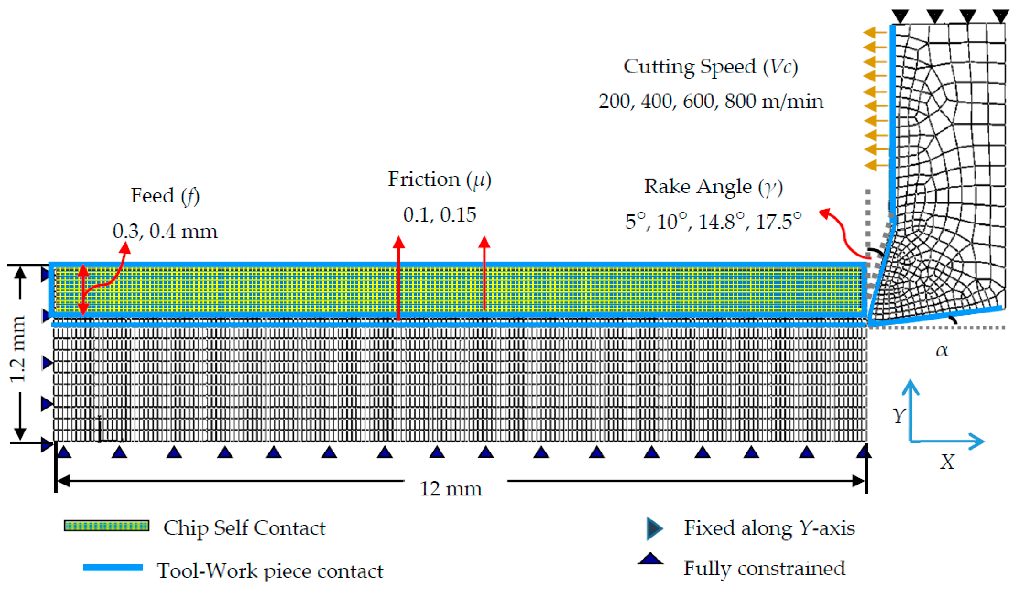
Figure 2. The work piece was developed into three sections: the chipped off material, the damage zone at tool-chip interface, and the uncut material. The configuration of the work piece into three different sections was essential to define different material properties, constitutive relationships, contact conditions, and the material damage laws. For example, JC material damage model and the damage evolution law were applied in the damage zone with a specific fracture energy; JC material damage model with a different fracture energy and the contact conditions were defined in the chipped off material; and the uncut material section was defined without JC damage parameters. The assembly of three parts was done by applying the standard join constraint (tie constraint) available in Abaqus. A tie constraint fuses the model surfaces with different mesh sizes and element types. Due to tie condition, each node at the slave surface attains the same displacement, stress, temperature, pressure, etc. corresponding to its closest node at the master surface. Tie condition makes the model computationally expensive and requires a compatible mesh between the part instances. Generally, Abaqus picks the slave surface with a finer mesh. For fidelity of the results of a multi-parts model assembled with the standard tie constraint, interested readers may refer to the online Abaqus documentation (tie constraints, Section 34.3.1, Abaqus Analysis User’s Manual) [49].
The model comprises 4134 four nodes quadrilateral continuum elements with plane strain (CPE4RT) and coupled temperature-displacement conditions. Cutting tool geometry consists of a nose radius (Rn) of 0.02 mm and a clearance angle 7°. A parametric sensitivity analysis was performed with different rake angles, cutting speeds, chip thickness, and the contact conditions to study the effect of tool rake angle on the chip temperature, the effect of contact friction on the cutting reaction force, the effect of cutting speeds on the equivalent plastic strain, the effect of feed upon the chip temperature, and the effect of friction coefficients on chip temperature. The cutting tool was constrained in y-direction and a self-contact was defined over the chip surface to avoid the penetration of deformed chip elements into the uncut chip and cutting tool. Contact conditions were established between the contact interfaces of the cutting tool, chip, damage zone, and the uncut material [50]. Selection of the proper friction coefficient and governing law is a critical and sensitive task in numerical cutting simulations. The friction characteristic at the tool-chip interface is difficult to determine since it is influenced by many factors; such as, the local cutting speed, contact pressure, temperature, cutting tool, work piece material, etc. [51]. An improper selection of the friction coefficient affects the results and findings. Extensive studies have been reported on the interaction of the tool-chip interface during the dry turning process. Several models have also been proposed to determine the contact friction. The most widely used method to determine the contact friction is Zorev’s stick-slip friction model [52] which is also known as an extended Columb’s law. In the present numerical simulations, the interaction between AA2024 material and the tungsten carbide tool insert, two different values of the friction coefficients (0.1 and 0.15) are used considering the similar experimental conditions [42] and also investigated by Zorev’s friction model.
Different properties and parameters used in the model are given in Table 1 [42]. The outcomes of turning simulations were compared with the available experimental results, given in Table 2 [
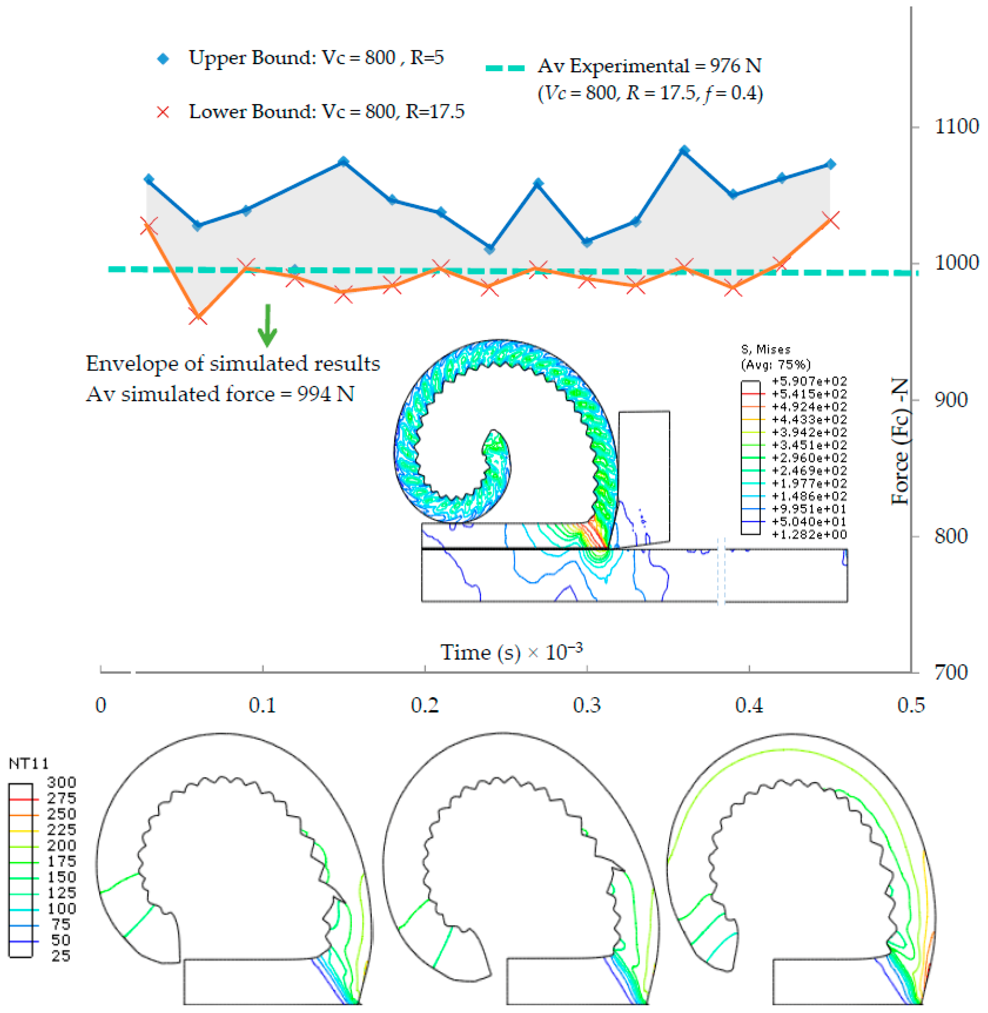
42]. Cutting force evolution and its comparison with the experimental results is shown in Figure 3. A summary of 64 cutting simulations is given in Table 3, where V is the cutting force (m/min); C is the feed (0.4 mm); F is the contact friction; RF (N) is the cutting reaction force; R (degrees) is the tool rake angle; and T is the temperature of the tool-chip interface. For further details, interested readers may consult the published work in Saleem et al. [42].

4.2. Artificial Neural Network (Modeling and Analysis)

The artificial neural network model adopted for this study is shown in 
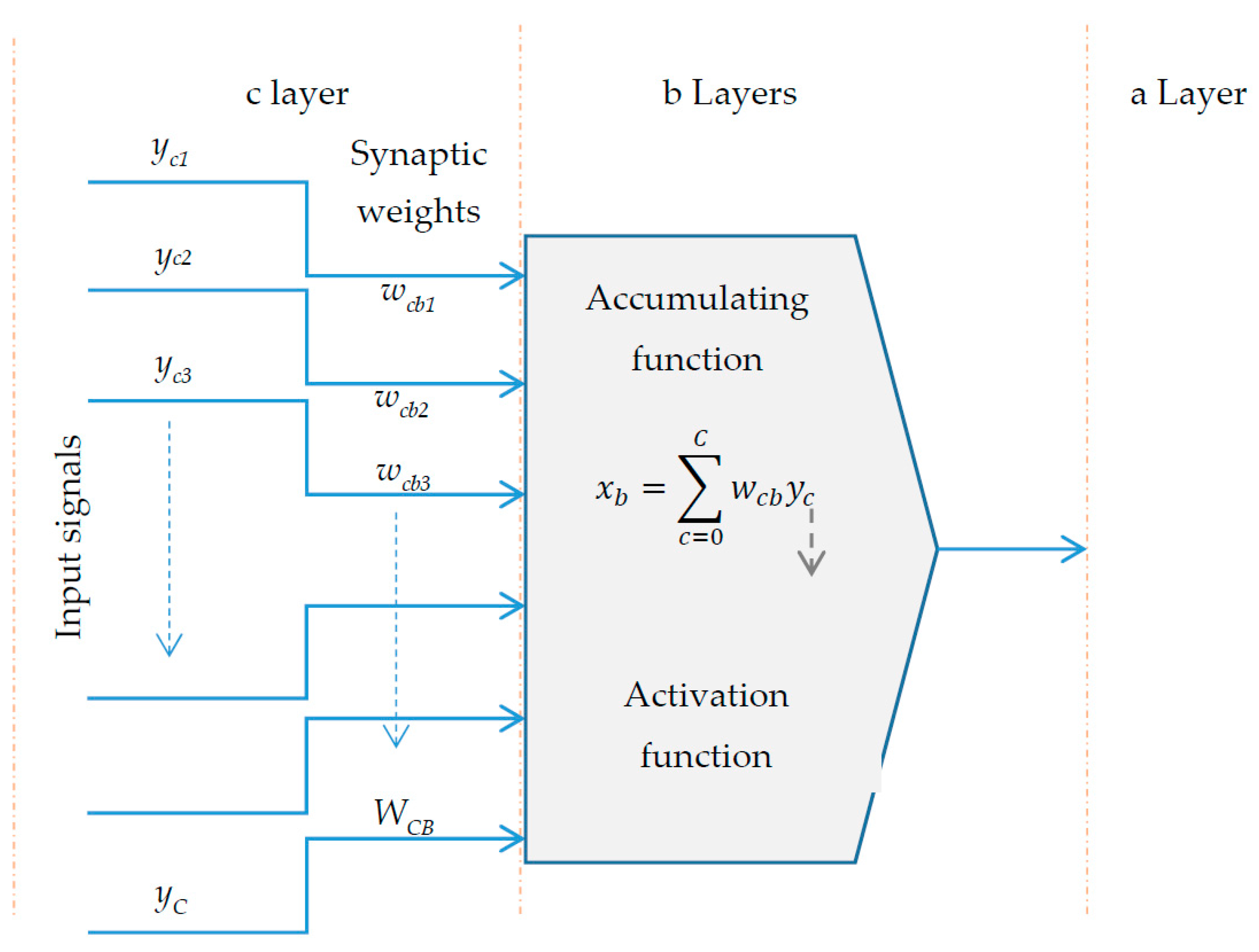
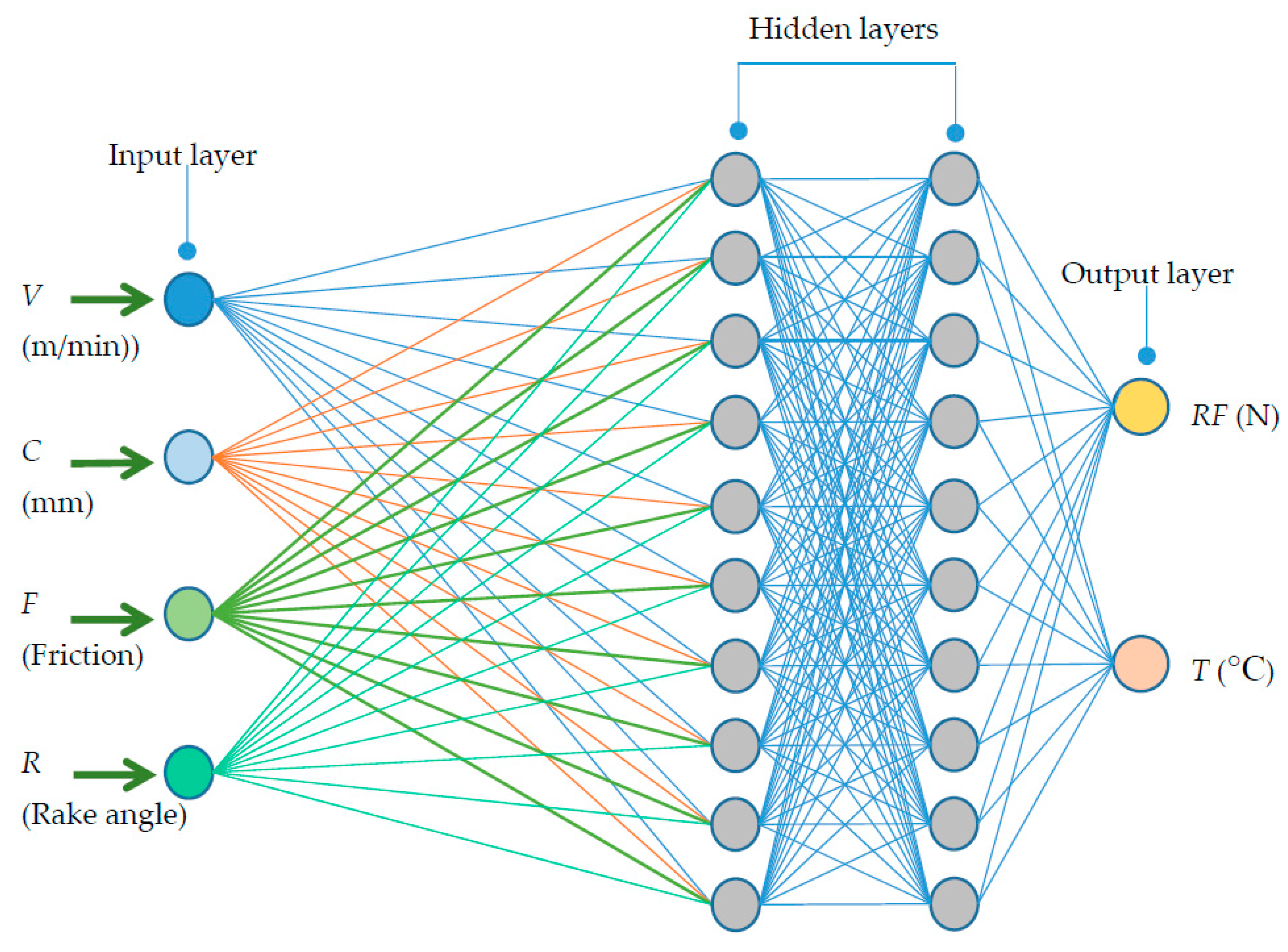
Figure 4. The model consists of three layers; the input layer, the hidden layer, and the output layer. The input parameters to the ANN model consist of the cutting parameters studied during the numerical simulations, and the outputs are the corresponding cutting reaction force and tool-chip interface temperature. The four input parameters consist of cutting force (V in m/min), cutting feed (C in 0.4 mm), contact friction (F), cutting reaction force (RF in Newtons), tool rake angle (R in degree), and the temperature at tool chip interface (T in °C). The output layer consists of two neurons: the cutting reaction force RF (N) and tool–chip interface temperature T (°C).
The MATLAB (R2013, The MathWorks, Natick, MA, USA, 2013), neural network toolbox was used for training and testing of the simulations data. Training of the network was accomplished by considering the 64 numerical simulations. The output (cutting reaction force and tool-chip interface temperature) and the corresponding input parameters of these simulations are given in Table 3. Design of the numerical experiments could also be accomplished with some standard technique (such as Taguchi’s configuration). In this research, different combinations of the input parameters were selected by considering the range of each parameter used in actual machining experiments. With four input parameters, all the possible combinations result into 4 × 4 × 2 × 2 = 64 design of numerical experiments.
Considering the available experimental data [42], the Abaqus simulations run at serial 13, 14, 16, 57, 58, and 60 were used for validation of the ANN model. The input parameters of these simulations are similar to the corresponding cutting conditions in actual experiments. The standard feedforward backpropagation neural network was studied by considering the Log-Sigmoid transfer function (LOGSIG). The Log-sigmoid transfer function is used for training the data in multi-layer networks with back-propagation algorithm [54,55,56]. The selection of optimal number of hidden layers is a difficult task. The optimal numbers of hidden layers are determined by training several networks and estimating the error. A few hidden layers may cause a high training error due to under-fitting and too many hidden layers may cause a high generalization error due to over-fitting. Selection also depends upon the numbers of input and output layers, learning function, the ANN architecture, the activation function, and the training algorithm. For the proposed ANN architecture, the numbers of neurons in the hidden layers were determined through a trial-and-error method. The best configuration was observed with two hidden layers and 10 neurons in each layer. The ANNs predicted outcomes and properties were evaluated by considering the mean-square-error and regression analysis. The predicted outcomes were validated with the published experimental results [42]. Details of the machining experiments, testing scheme, and the measurement techniques are described in the published article. The ANN parameters for training and testing are given in Table 4.
The default Levenberg-Marquardt algorithm was used for training the network. The maximum validation checks (max_fail) function was taken as 6. This parameter (max_fail) serves as a training function parameter and ensures the maximum number of validation checks before the training is stopped. Therefore, it must be a positive integer. The validation fails are total successive iterations that the validation performance fails to decrease or when the validation MSE (mean-square-error) increases the max_fail value. This criterion can be changed by setting the parameter net.trainParam.max_fail. A large number of trainings show the over training and Matlab tries to stop the training after 6 failed in a row. In the back-propagation, the learning rate and the momentum factor are very significant to determine the learning speed and accuracy [57]. The learning rate controls the changes in the weights during the training process. The momentum factor manages the speed of network training. It defines the fraction of preceding weight changes to be included in the current weight changes. Termination of the training depends upon the magnitude of the gradient and the number of validation checks. In case, when the training reaches the minimum of the performance, the gradient becomes very small. For example, the training stops when the magnitude of the gradient is less than 1 × 10⁻⁵. This limit can be adjusted by setting the parameter net.trainParam.min_grad.
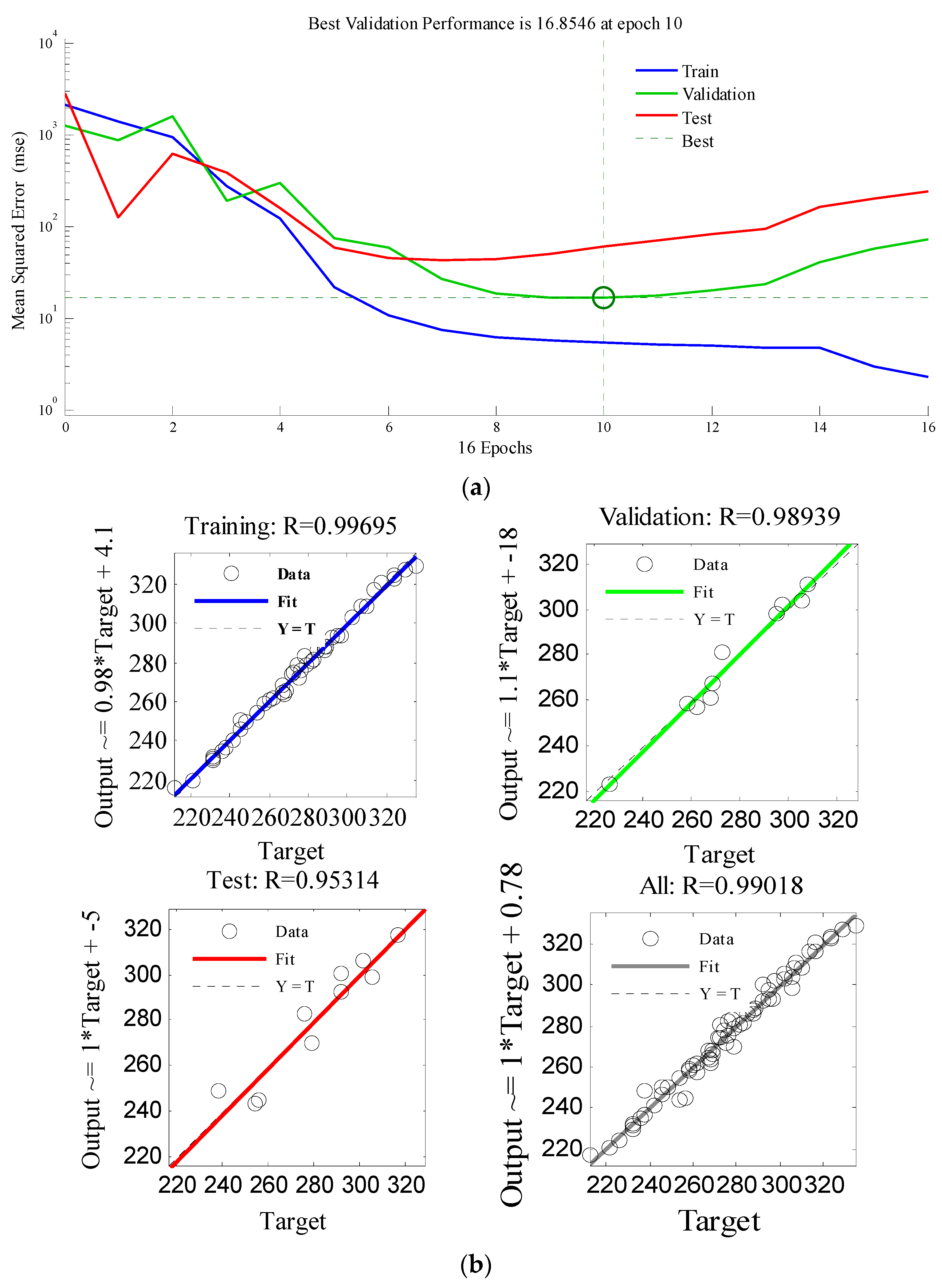
Figure 5a shows the performance, training statistics, and the convergence plots for testing and training networks of tool-chip interface temperature. The performance plot (mean square error of all data sets) is shown on a logarithmic scale. The training mean square error must show a decreasing trend. Here, the training plot shows a perfect training. The other two plots explain the network simulation results after the training. The training was terminated when the validation error increased to 16 epochs, and the best validation performance was obtained as 16.58 at 10th epoch. The test set error and the validations set error have also shown the similar characteristics. Figure 5b shows the coefficients of regression. The R-plots explain the significance between the target (desired output) and the ANN output (actual output). The dashed line in each plot represents the targeted values (the difference between the perfect result and outputs). The best-fit linear regression line between the outputs and targets is represented by a solid line. The correlation coefficient (R) gives the relationship between the outputs and the targets.
The maximum value of the correlation coefficient (R2) and a minimum value of the root mean square error defines a good ANN model. For an exact linear relationship, R must be closer or equal to one. The values of coefficients for training and testing data are founded to be 0.996 and 0.953, respectively. For a perfect fit, the distribution of data should be along a 45° line, which shows that the network outputs are equal to the targets. From Figure 5b, it was observed that the targeted output R for training is 0.99695, validation is 0.98939), and testing is 0.95314. The corresponding total response is 0.999018. R = 0.999018 verifies that the ANN output perfectly matches with the target (precise linear relevance). The overall response verifies that the training has produced the optimal results, and the model can entertain the new inputs. Values of all the coefficients are very close to 1, so the training value is highly acceptable. 
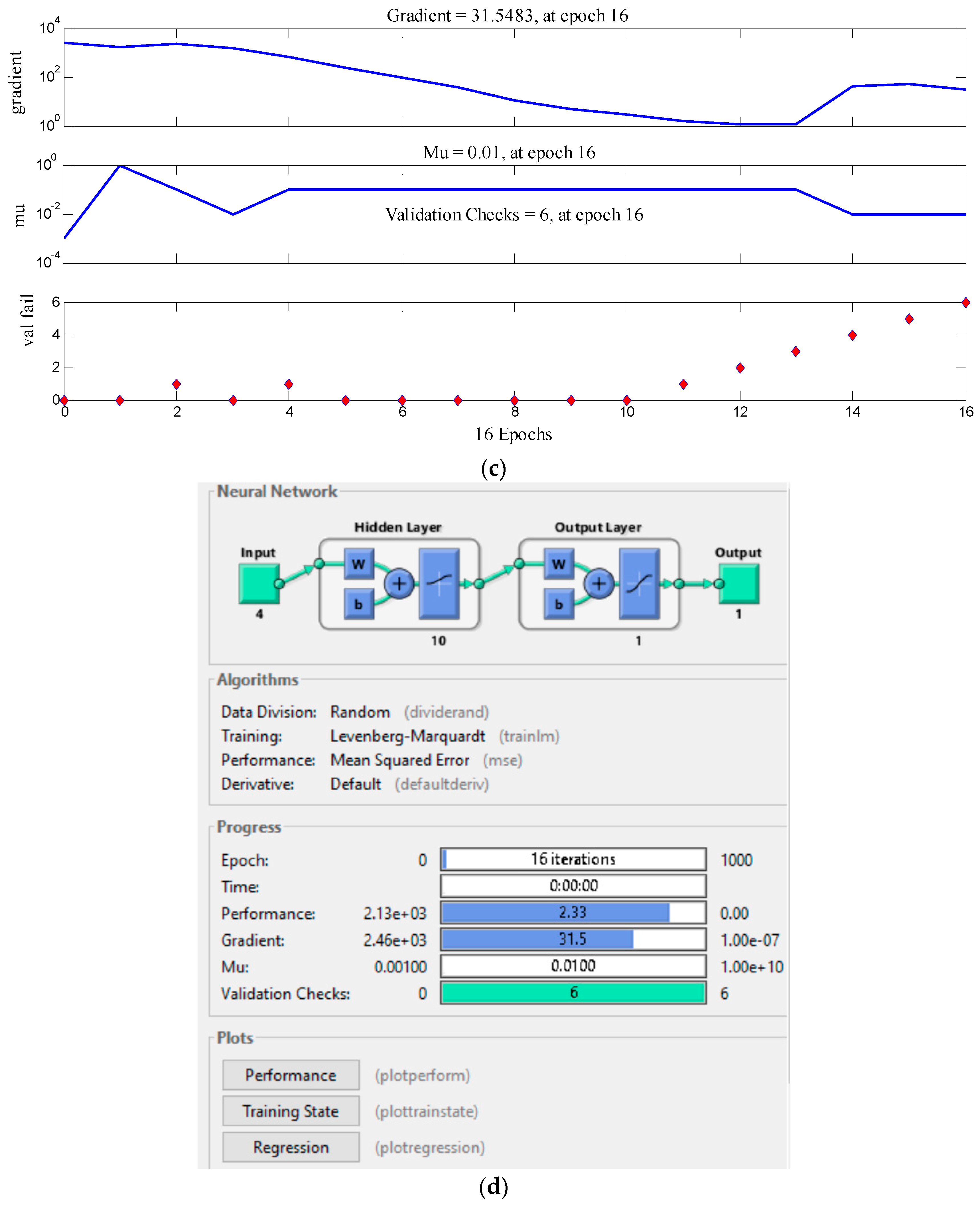
Figure 5d is a caption window that shows the validation of ANN model and also explains the output of the neural network during the training and training developments. Figure 5c shows the model evolution, validation, and the corresponding gradient of epochs. For the temperature prediction model, the gradient of epochs was attained as 31.548.
The second ANN model for cutting reaction force was developed by keeping the same input parameters, as shown in Figure 4. The ANN parameters for training and testing are presented in Table 4. The training and performance evaluation of the network was accomplished with 64 data sets, given in Table 3. The standard feedforward backpropagation neural network was considered with Log-Sigmoid transfer function (LOGSIG) and Levenberg-Marquardt algorithm. The optimized network was detected with 10 neurons in the hidden layers. The ANN predicted outcomes were evaluated by comparing with the published experimental results [42]. The ANN predicted values and the performance curves of cutting reaction force are shown in
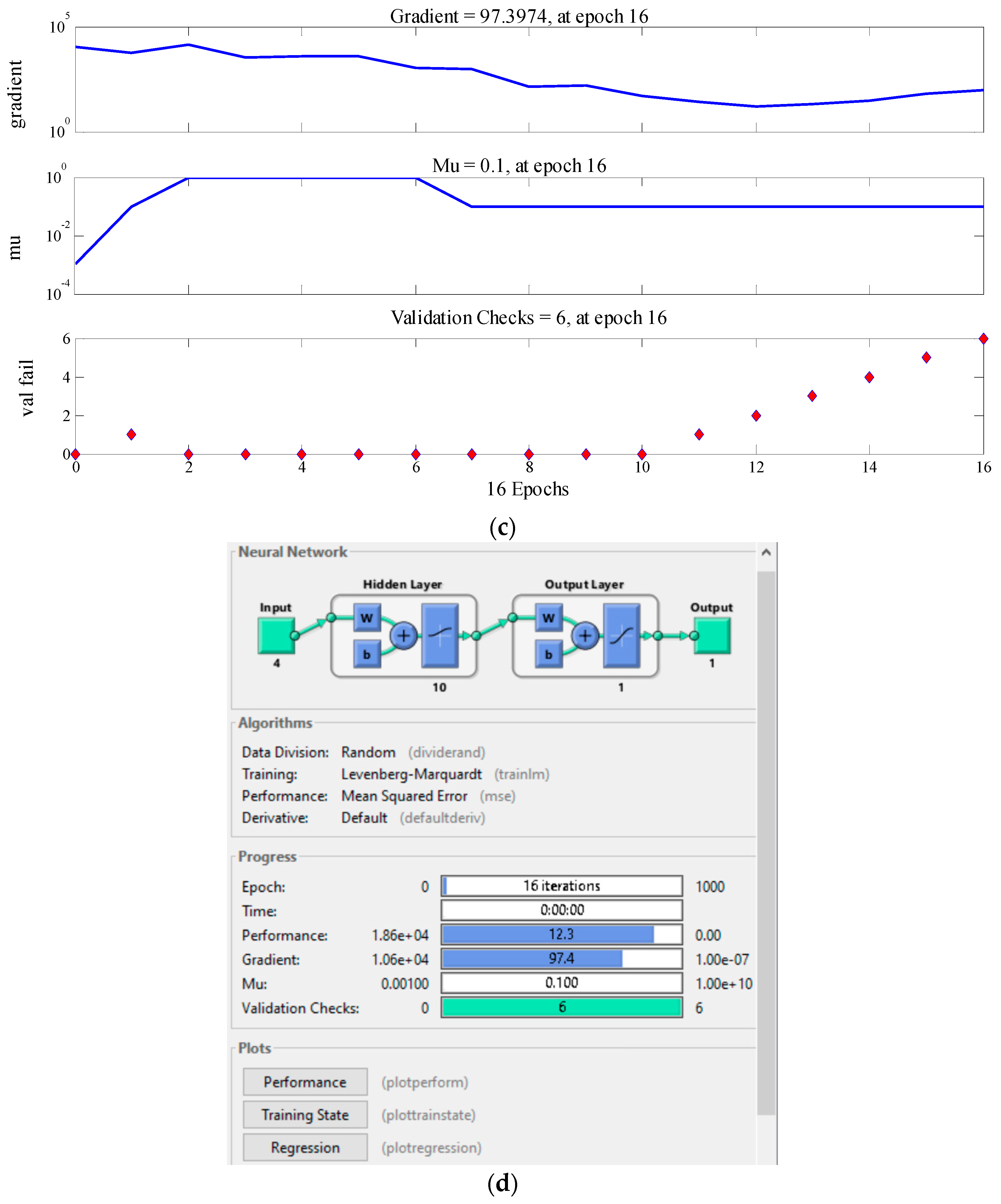
 Figure 6a–d. Figure 6a illustrates the performance, training statistics, and the convergence plots for training the network. The performance curve shown in Figure 6a demonstrates a perfect training; the test set error, and the validation set error plots also interpret the similar characteristics. Training was completed when the validation error increased to 16 epochs, and the best validation performance was attained as 57.4402 at 10th epoch. The regression analysis is shown in Figure 6b. The coefficients of regression value for training and testing data were attained as 0.99801 and 0.96738, respectively. The targeted output value of the validation and corresponding total response are 0.99512 and 0.98768, respectively. The overall results demonstrate a precise linear relevance and validate the model for accommodating the new inputs and simulating the final results. Figure 5c illustrates the model validation and the corresponding gradient of epochs. The gradient of epochs was attained as 97.3974. The network configuration, the optimization scheme, and the validation of ANN model are shown as a caption window in Figure 6d.
A comparison of the numerical simulation results with the ANN predicted values is presented in Table 5. The term RF_Pd gives the predicted reaction force, Err is the error, % Err is the percent error, T is the chip-tool interface temperature, and T_Pd is the chip-tool interface predicted temperature. The performance of the ANN model elaborates the deviation (error) between the actual and predicted values. In Table 5, the maximum percentage errors of the cutting reaction force and the chip-tool interface temperature are found to be 2.55 and 3.34, respectively. The calculated errors are found reasonable and demonstrate the conformance of ANN predicted results.
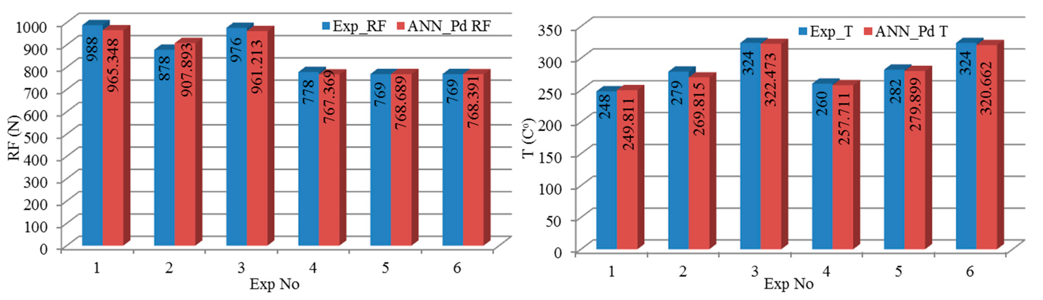
The ANN predicted values of tool-chip interface temperatures and reaction forces were compared with the experimental results [42,58]. Values are presented in Table 6, where the term % Err shows the percent error; ANN_Sim RF is the ANN simulated reaction force; Exp_RF is the experimental value of the reaction force; ANN_Sim T is the ANN simulated temperature; and Abq Sim_T is the Abaqus simulated chip–tool interface temperature. The ANN simulated values of cutting reaction force and tool–chip interface temperatures are found in good approximation with the experimental results [42]. This shows that the ANN models developed for the temperature and reaction force can be used effectively for predicting the optimal parameters. The maximum percentage errors for ANN predicted reaction force and the chip–tool interface temperatures are 3.4 and 3.2, respectively. Figure 7 implies a good agreement between experimental and ANN simulated outcomes.

5. Conclusions

In this study, the dry turning process parameters (cutting speed, feed rate, tool rake angle, and contact friction coefficient) were investigated through Abaqus/Explicit numerical simulations and optimized with ANN models. The ANN predicted outcomes demonstrated that the designed intelligence models produced the reliable training data. Subsequently, training data were used to simulate the optimum cutting parameters. The maximum percentage errors between the ANN predicted and experimental results for the cutting reaction force and temperature are found to be 2.55 and 3.34, respectively. The small errors validate the conformance of ANN predictive models. The coefficients of regression for training, testing, and validation data showed a perfect linear relationship and closer to one. The performance curves and regression analysis of both models represent the consistency of the solution. The presented research demonstrates that an integrated ANN-FEM approach can be applied effectively to predict the reliable turning process parameters.

Author Contributions

Waqas Saleem, Muhammad Zain-ul-abdein, Tarek Mabrouki, and Hassan Ijaz worked on the numerical modeling and cutting simulations. Muhammad Asad suggested the material behavior laws and performed the turning experiments. Abdullah Salmeen Bin Mahfouz and Anas Ahmed worked on the Artificial Neural Networks and supervised the overall project. Tarek Mabrouki, and Waqas Saleem compiled the results. The co-authors assisted in preparing the revised versions and proof-read the final manuscript.

Conflicts of Interest

The authors declare no conflict of interest.

Nomenclature

γtool rake angle
Vccutting velocity
fcutting feed
μcontact friction coefficient
σ ¯ equivalent stress
Amaterial yield strength (MPa) at room temperature
Bmaterial hardening modulus
nwork hardening exponent
Cmaterial constant for strain hardening rate
mthermal softening coefficient
Troomreference ambient temperature
Tmeltmelting temperature
ε ¯ equivalent plastic strain
Δ ε ¯ increment of equivalent plastic strain during damage evolution
ε f ¯ equivalent strain to fracture
D1initial failure strain
D2exponential factor
D3triaxiality factor
D4strain rate factor
D5temperature factor
Paverage normal stress
Emodulus of elasticity of material
υPoisson ratio
qpheat generation rate
ηpinelastic heat fraction
τfshear stress by Coulomb friction law
ε ¯ ˙ plastic strain rate
ε ¯ ˙ o reference strain rate
Wsynaptic weights
yinput signals to the respective neutron’s
aoutput layer of ANN
bhidden layer of ANN
trepresents a target value (desired activation)
Eerror
Alearning rate
Niteration (epoch)
Ηmomentum
RFreaction force
RF_Pdpredicted reaction force
Errerror
% Errpercent error
Tchip-tool interface temperature
T_Pdchip-tool interface predicted temperature
ANN_Sim RFANN simulated reaction force
Exp_RFExperimental value of reaction force
ANN_Sim TANN simulated temperature
Abq Sim TAbaqus simulated chip-tool interface temperature

References

  1. Fang, N.; Wu, Q. The effects of chamfered and honed tool edge geometry in machining of three aluminium alloys. Int. J. Mach. Tool Manuf. 2005, 45, 1178–1187. [Google Scholar] [CrossRef]
  2. Klocke, F.; Raedt, H.W.; Hoppe, S. 2D-FEM Simulation of the orthogonal high speed cutting process. Mach. Sci. Technol. 2006. [Google Scholar] [CrossRef]
  3. Johnson, G.R.; Cook, W.H. Fracture characteristics of three metals subjected to various strains, strain rates, temperatures and pressures. Eng. Fract. Mech. 1985, 21, 31–48. [Google Scholar] [CrossRef]
  4. Lo, S.P. An analysis of cutting under different rake angles using the finite element method. J. Mater. Process. Technol. 2000, 105, 43–151. [Google Scholar] [CrossRef]
  5. Sutter, G. Chip geometries during high-speed machining for orthogonal cutting conditions. Int. J. Mach. Tool Manuf. 2005, 45, 719–726. [Google Scholar] [CrossRef]
  6. Dahlman, P.; Gunnberg, F.; Jacobson, M. The influence of rake angle, cutting feed and cutting depth on residual stresses in hard turning. J. Mater. Process. Technol. 2004, 147, 181–184. [Google Scholar] [CrossRef]
  7. Attanasio, A.; Ceretti, E.; Giardini, C. 3D FE Modelling of superficial residual stresses in turning operations. Mach. Sci. Technol. 2009, 13, 317–337. [Google Scholar] [CrossRef]
  8. Yanda, H.; Ghani, J.A.; Haron, C.H.C. Effect of rake angle on stress, strain and temperature on the edge of carbide cutting tool in orthogonal cutting using fem simulation. ITB J. Eng. Sci. 2010, 42, 179–194. [Google Scholar] [CrossRef]
  9. Axinte, D.A.; Belluco, W.; Chiffre, L.D. Evaluation of cutting force uncertainty components in Turning. Int. J. Mach. Tool Manuf 2001, 41, 719–730. [Google Scholar] [CrossRef]
  10. Saglam, H.; Unsacar, F.; Yaldiz, S. Investigation of the effect of rake angle and approaching angle on main cutting force and tool tip temperature. Int. J. Mach. Tool Manuf. 2006, 46, 132–141. [Google Scholar] [CrossRef]
  11. Shi, G.; Xiaomin, D.; Shet, C. A finite element study of the effect of friction in orthogonal metal cutting. Finite Elem. Anal. Des. 2002, 38, 863–883. [Google Scholar] [CrossRef]
  12. Zhang, Y.C.; Mabrouki, T.; Nelias, D.; Gong, Y.D. Chip formation in orthogonal cutting considering interface limiting shear stress and damage evolution based on fracture energy approach. Finite Elem. Anal. Des. 2011, 47, 850–863. [Google Scholar] [CrossRef]
  13. Neseli, S.; Yaldiz, S.; Turkes, E. Optimization of tool geometry parameters for turning operations based on the response surface methodology. Measurement 2011, 44, 580–587. [Google Scholar] [CrossRef]
  14. Dogu, Y.; Aslan, E.; Camuscu, N. A numerical model to determine temperature distribution in orthogonal metal cutting. J. Mater. Process. Technol. 2006, 171, 1–9. [Google Scholar] [CrossRef]
  15. D’Addona, D.M.; Teti, R. Genetic algorithm-based optimization of cutting parameters in turning processes. Procedia CIRP 2013, 7, 323–328. [Google Scholar] [CrossRef]
  16. Marko, H.; Simon, K.; Tomaz, I.; Matej, P.; Joze, B.; Miran, B. Turning parameters optimization using particle swarm optimization. Procedia Eng. 2014, 69, 670–677. [Google Scholar] [CrossRef]
  17. Prasanth, R.S.S.; Raj, K.H. Optimization of straight cylindrical turning using Artificial Bee Colony (ABC) algorithm. J. Inst. Eng. Ser. C 2012, 98, 171–177. [Google Scholar] [CrossRef]
  18. Amer, F.Z.; El-Garhy, A.M.; Awadalla, M.H.; Rashad, S.M.; Abdien, A.K. A real-valued genetic algorithm to optimize the parameters of support vector machine for classification of multiple faults in NPP. Nukleonika 2011, 56, 323–332. [Google Scholar]
  19. Bruni, C.; D’Apolito, L.; Forcellese, A.; Gabrielli, F.; Simoncini, M. Surface roughness modelling in finish face milling under MQL and dry cutting conditions. Int. J. Mater. Form. 2008, 1, 503–506. [Google Scholar] [CrossRef]
  20. Sick, B. On-line and indirect tool wear monitoring in turning with artificial neural networks: A review of more than a decade of research. Mech. Syst. Signal 2002, 16, 487–546. [Google Scholar] [CrossRef]
  21. Ezugwu, E.O.; Fadare, D.A.; Bonney, J.; Da Silva, R.B.; Sales, W.F. Modelling the correlation between cutting and process parameters in high-speed machining of Inconel 718 alloy using an artificial neural network. Int. J. Mach. Tools Manuf. 2005, 45, 1375–1385. [Google Scholar] [CrossRef]
  22. Correa, M.; Bielza, C.; Pamies-Teixeira, J. Comparison of bayesian networks and artificial neural networks for quality detection in a machining process. Expert Syst. Appl. 2009, 36, 7270–7279. [Google Scholar] [CrossRef]
  23. Çaydas, U.; Hasçalik, A. A study on surface roughness in abrasive waterjet machining process using artificial neural networks and regression analysis method. J. Mater. Process. Technol. 2008, 202, 574–582. [Google Scholar] [CrossRef]
  24. Mahmoodkhani, Y.; Wells, M.A.; Song, G. Prediction of roll force in skin pass rolling using numerical and artificial neural network methods. Ironmak. Steelmak. 2017, 44, 281–286. [Google Scholar] [CrossRef]
  25. Ranganathan, S.; Senthilvelan, T.; Sriram, G. Evaluation of machining parameters of hot turning of stainless steel (type 316) by applying ANN and RSM. Mater. Manuf. Processes 2010, 25, 1131–1141. [Google Scholar] [CrossRef]
  26. Chang, C.K.; Lu, H.S. Study on the prediction model of surface roughness for side milling operations. Int. J. Adv. Manuf. Technol. 2006, 29, 867–878. [Google Scholar] [CrossRef]
  27. Pal, S.K.; Chakraborty, D. Surface roughness prediction in turning using artificial neural network. Neural Comput. Appl. 2005, 14, 319–324. [Google Scholar] [CrossRef]
  28. Cus, F.; Zuperl, U. Approach to optimization of cutting conditions by using artificial neural networks. J. Mater. Process. Technol. 2007, 173, 281–290. [Google Scholar] [CrossRef]
  29. Reddy, N.S.K.; Rao, P.V. Selection of optimum tool geometry and cutting conditions using a surface roughness prediction model for end milling. Int. J. Adv. Manuf. Technol. 2005, 26, 1202–1210. [Google Scholar] [CrossRef]
  30. Umbrello, D.; Ambrogio, G.; Filice, L.; Shivpuri, R.A. Hybrid finite element method-artificial neural network approach for predicting residual stresses and the optimal cutting conditions during hard turning of AISI 52100 bearing steel. Mater. Des. 2008, 29, 873–883. [Google Scholar] [CrossRef]
  31. Haykin, S. Neural Networks A Comprehensive Foundation, 2nd ed.; Pearson: McMaster University, Hamilton, ON, Canada, 1999. [Google Scholar]
  32. Hopfield, J.J. Neural networks and physical systems with emergent collective properties. Proc. Natl. Acad. Sci. USA 1982, 79, 2554–2558. [Google Scholar] [CrossRef] [PubMed]
  33. Kohonen, T. Self-organized formation of topologically correct feature maps. Biol. Cybern. 1982, 43, 59–69. [Google Scholar] [CrossRef]
  34. Minsky, M.; Papert, S.A. Perceptrons; MIT Press: Cambrige, UK, 1969. [Google Scholar]
  35. Salakhutdinov, R.; Hinton, G. A better way to pretrain deep boltzmann machines. In Advances in Neural Information Processing Systems 25 (NIPS 2012); MIT Press: San Diego, CA, USA, 2012; Volume 25. [Google Scholar]
  36. Konstantinos, K.; Kalouptsidis, N. Generalized hamming networks and applications. Neural Netw. 2005, 18, 896–913. [Google Scholar]
  37. Hu, X.; Duan, S.; Chen, G.; Chen, L. Modeling affections with memristor-based associative memory neural networks. Neurocomputing 2017, 223, 129–137. [Google Scholar] [CrossRef]
  38. Kuzmanovski, I.; Novic, M. Counter-propagation neural networks in Matlab. Chemom. Intell. Lab. Syst. 2008, 90, 84–91. [Google Scholar] [CrossRef]
  39. Diamantopoulou, M.J.; Georgiou, P.E.; Papamichail, D.M. A time delay artificial neural network approach for flow routing in a river system. Hydrol. Earth Syst. Sci. 2006, 3, 2735–2756. [Google Scholar] [CrossRef]
  40. Pai, T.Y.; Chuang, S.H.; Ho, H.H.; Yu, L.F.; Su, H.C.; Hu, H.C. Predicting performance of grey and neural network in industrial effluent using online monitoring parameters. Proc. Biochem. 2008, 43, 199–205. [Google Scholar] [CrossRef]
  41. Basheer, I.A.; Hajmeer, M. Artificial neural networks: Fundamentals, computing, design, and application. J. Microbiol. Method 2000, 43, 3–31. [Google Scholar] [CrossRef]
  42. Asad, M. Elaboration of Concepts and Methodologies to Study Peripheral Down-Cut Milling Process from Macro-to-Micro Scales. Ph.D. Thesis, INSA, Lyon, France, 2011. [Google Scholar]
  43. Umbrello, D. Finite element simulation of conventional and high speed machining of Ti–6Al–4V alloy. J. Mater. Process. Technol. 2008, 196, 79–87. [Google Scholar] [CrossRef]
  44. Han, Z.Y.; Huang, X.G.; Cao, Y.G.; Xu, J.Q. A nonlinear cumulative evolution model for corrosion fatigue damage. J. Zhejiang Univ. Sci. A 2014, 15, 447–453. [Google Scholar] [CrossRef]
  45. Zhang, X.; Wu, S.; Wang, H.; Liu, C.R. Predicting the effects of cutting parameters and tool geometry on hard turning process using finite element method. J. Manuf. Sci. Eng. 2011, 133, 041010. [Google Scholar] [CrossRef]
  46. Hillerborg, A.; Modeer, M.; Petersson, P.E. Analysis of crack formation and crack growth in concrete by means of fracture mechanics and finite elements. Cem. Concr. Res. 1976, 6, 773–781. [Google Scholar] [CrossRef]
  47. Baker, M. Finite element investigation of the flow stress dependence of chip formation. J. Mater. Proc. Technol. 2005, 167, 1–13. [Google Scholar] [CrossRef]
  48. Rumelhart, D.E.; Hinton, G.E.; Williams, R.J. Learning Internal Representations by Error Propagation, Parallel Distributed Processing: Explorations in the Microstructures of Cognition; Foundations: Chapter 8; MIT Press: Cambridge, UK, 1986; Volume I. [Google Scholar]
  49. Abaqus Online Documentation. Available online: https://engrapache01.engineering.iastate.edu/abaqus/Documentation/docs/v6.14/books/usb/default.htm?startat=pt08ch35s06aus138.html (accessed on 7 June 2017).
  50. Li, K.; Gao, X.L.; Sutherland, J.W. Finite element simulation of the orthogonal metal cutting process for qualitative understanding of the effects of crater wear on the chip formation process. J. Mater. Process. Technol. 2002, 127, 309–324. [Google Scholar] [CrossRef]
  51. Zemzemi, F.; Rech, J.; Salem, W.B.; Dogui, A.; Kapsa, P. identification of a friction model at the tool-chip-workpiece interfaces in dry cutting of an inconel 718 alloy with cbn and coated carbide tools. Adv. Manuf. Sci. Technol. 2014, 38, 5–22. [Google Scholar] [CrossRef]
  52. Zorev, N.N. Inter-relationship between shear processes occurring along tool face and shear plane in metal cutting. Int. Res. Prod. Eng. 1963, 49, 143–152. [Google Scholar]
  53. Saleem, W.; Asad, M.; Zain-ul-abdein, M.; Ijaz, H.; Mabrouki, T. Numerical investigations of optimum turning paramters-AA2024T351 Aluminum alloy. J. Mach. Sci. Technol. 2016, 20, 634–654. [Google Scholar] [CrossRef]
  54. Dawson, C.W.; Wilby, R.L.; Dawson, C.W. Hydrological modelling using artificial neural networks. Prog. Phys. Geogr. 2001, 25, 80–108. [Google Scholar] [CrossRef]
  55. Yonaba, H.; Anctil, F.; Fortin, V. Comparing sigmoid transfer functions for neural network multistep ahead streamflow forecasting. J. Hydrol. Eng. ASCE 2010, 15, 275–283. [Google Scholar] [CrossRef]
  56. Dorofki, M.; Elshafie, A.H.; Jaafar, O.; Karim, O.A.; Mastura, S. Comparison of artificial neural network transfer functions abilities to simulate extreme runoff data. In International Proceedings of Chemical, Biological and Environmental Engineering IPCBEE; IACSIT Press: Singapore, 2012; Volume 33. [Google Scholar]
  57. Attoh-Okine, N.O. Analysis of learning rate and momentum term in backpropagation neural network algorithm trained to predict pavement performance. Adv. Eng. Softw. 1999, 30, 291–302. [Google Scholar] [CrossRef]
  58. Ni, W.; Cheng, Y.T.; Weiner, A.M.; Perry, T.A. Tribological behaviour of diamond-like carbon (DLC) coatings against aluminium alloys at elevated temperatures. Surf. Coat. Technol. 2006, 201, 3229–3234. [Google Scholar] [CrossRef]
Figure 1. Basic architecture of an ANN.
Applsci 07 00642 g001
Figure 2. Turning simulations model.
Applsci 07 00642 g002
Figure 3. Parametric sensitivity analysis (cutting reaction force (N), chip stress (MPa), and tool-chip interface temperate (°C)) [53].
Applsci 07 00642 g003
Figure 4. ANN model for cutting simulations.
Applsci 07 00642 g004
Figure 5. (a) Neural network performance plot for tool-chip interface temperature (T); (b) Neural network regression plots for chip-tool interface temperature (T); (c) Neural network performance and gradient epochs (chip-tool interface temperature); (d) Neural training and the output window for chip-tool interface temperature (T).
Applsci 07 00642 g005aApplsci 07 00642 g005b
Figure 6. (a) Neural network performance plot for cutting reaction force (RF); (b) Neural network regression plots for cutting reaction force (RF); (c) Neural network performance and gradient epochs for cutting reaction force (RF); (d) Neural training and output window for cutting reaction force (RF).
Applsci 07 00642 g006aApplsci 07 00642 g006b
Figure 7. Comparison of experimental [42] and ANN simulated results.
Applsci 07 00642 g007
Table 1. Work piece and cutting tool properties.
Physical Parameters
PropertyWork Piece (A2024-T351)Tool (Tungsten Carbide)
Density, ρ (Kg/m3)270011,900
Elastic modulus, E (Gpa)73534
Poisson ratio, ν0.330.22
Specific heat, Cp (J·Kg−1·°C−1)Cp = 0.557T + 877.6400
Thermal conductivity, λ (W·m−1·C−1)25 ≤ T ≤ 300: λ = 0.247T + 114.4
300 ≤ TTmelt: λ = −0.125T + 226.0
50
Expansion, α (µmm−1·°C−1)α + 8.9 × 10⁻³T + 22.2-
Tmelt (°C)520-
Troom (°C)2525
Johnson-Cook Material Parameters (Identified for A2024-T351)
A (MPa)B (Mpa)nCmD1D2D3D4D5
3524400.420.008310.130.13−1.50.0110
Table 2. Experimental results—Turning AA2024 [42].
Feed, f (mm)ParameterCutting Speed, V (m/min)
200400800
0.3Force778 N769 N769 N
Frequency128 Hz290 Hz/37.8 kHz500 Hz/90.7 kHz
0.4Force988 N978 N976 N
Frequency120 Hz/10.3 kHz351 Hz/32.4 kHz889 Hz/64.8 kHz
0.5Force1216 N1196 N1192 N
Frequency256 Hz/16.2 kHz476 Hz/22.7 kHz1026 Hz/45.3 kHz
Table 3. Parametric sensitivity analysis (turning simulations).
S No.VCFRRFTS No.VCFRRFT
12000.40.15500226332000.30.110790236
24000.40.15600256344000.30.110800262
36000.40.15650269356000.30.110990273
48000.40.15700288368000.30.1101000302
52000.40.110800232372000.30.1510800232
64000.40.110700262384000.30.1510870258
76000.40.110650276396000.30.1510590285
88000.40.110490292408000.30.1510780306
92000.40.114.8700246412000.40.1514.8750246
104000.40.114.8800267424000.40.1514.8775275
116000.40.114.8600279436000.40.1514.8870289
128000.40.114.8550307448000.40.1514.8900317
132000.40.117.5790248452000.30.114.8790238
144000.40.117.5795279464000.30.114.8800269
156000.40.117.5870292476000.30.114.8990274
168000.40.117.5895324488000.30.114.81000310
172000.40.155750232492000.30.1514.8800258
184000.40.155775254504000.30.1514.8870283
196000.40.155870292516000.30.1514.8590302
208000.40.155900308528000.30.1514.8780317
212000.30.15790221532000.40.1517.5750268
224000.30.15800254544000.40.1517.5775278
236000.30.15990267556000.40.1517.5870298
248000.30.151000288568000.40.1517.5900329
252000.30.155800212572000.30.117.5790260
264000.30.155870242584000.30.117.5800282
276000.30.155590273596000.30.117.5990295
288000.30.155780295608000.30.117.51000324
292000.40.1510750238612000.30.1517.5800272
304000.40.1510775268624000.30.1517.5870297
316000.40.1510870276636000.30.1517.5590314
328000.40.1510900306648000.30.1517.5780335
Table 4. ANN network and training parameters.
FunctionValueDescription
Training function-TRAINLM
Adaptation learning function-LEARNGDM
Network type-Feed-forward backprop
Transfer function-LOGSIG
net.trainParam.epochs1000Maximum number of epochs to train
net.trainParam.goal0Performance goal
net.trainParam.showCommandLinefalseGenerate command-line output
net.trainParam.showWindowtrueShow training GUI
net.trainParam.lr0.01Learning rate
net.trainParam.max_fail6Maximum validation failures
net.trainParam.min_grad1 × 10−7Minimum performance gradient
net.trainParam.show25Epochs between displays
net.trainParam.timeinfMaximum time to train in seconds
Table 5. ANN predicted results for cutting reaction force and tool-chip interface temperature.
SrRFRF_PdErr% ErrTT_PdErr% ErrSrRFRF_PdErr% ErrTT_PdErr% Err
1894895.142−1.1420.13226223.7422.2581.0133759765.873−6.8730.90236235.2830.7170.30
2897895.5481.4520.16253244.8298.1713.3434763768.117−5.1170.67262262.117−0.1170.04
3889890.221−1.2210.14269267.9091.0910.4135758766.854−8.8541.15273280.794−7.7942.78
4902901.5910.4090.05288288.045−0.0450.0236766759.7776.2230.82302302.936−0.9360.31
5932930.2031.7970.19232232.349−0.3490.1537749750.858−1.8580.25232229.8722.1280.93
6916917.691−1.6910.18262257.4644.5361.7638747751.467−4.4670.59258258.786−0.7860.30
7940943.037−24.0372.55276275.4710.5290.1939755749.1175.8830.79285286.262−1.2620.44
8927927.464−0.4640.05292300.272−8.2722.7540761761.831−0.8310.11306298.7317.272.43
9941947.089−6.0890.64246246.158−0.1580.0641782784.039−2.0390.26246250.562−4.5621.82
10961967.501−6.5010.67267264.6832.3170.8842788786.7561.2440.16275271.8513.1491.16
11966967.813−1.8130.19279279.071−0.0710.0343802793.7988.2021.03289288.3910.6090.21
12961961.414−0.4140.04307308.542−1.5420.5044795792.962.040.26317316.9460.0540.02
13972965.3486.6520.69248249.811−1.8110.7245769766.9232.0770.27243248.703−5.7032.29
14963967.893−4.8930.51279269.8159.1853.4046766768.563−2.5630.33269265.9573.0431.14
15969966.9362.0640.21292292.275−0.2750.0947772768.5873.4140.44274278.352−4.3521.56
16968961.2136.7870.71324322.4731.5270.4748771766.8944.1060.54310308.1931.8070.59
17809808.8940.1060.01232230.9531.0470.4549769760.9258.0751.06258258.4−0.40.15
18793794.405−1.4050.18254254.239−0.2380.0950764760.1613.8390.51283281.5651.4350.51
19789797.68−8.681.09292292.763−0.7630.2651769772.293−3.2930.43302306.103−4.1031.34
20803808.702−5.7020.71308311.076−3.0760.9952777772.4934.5070.58317320.696−3.6961.15
21791789.7751.2250.16221220.1450.8550.3953758757.2140.7860.10268263.8944.1061.56
22807812.016−5.0160.62250243.5146.4862.6654749751.408−2.4080.32278283.013−5.0131.77
23812813.088−1.0880.13267268.369−1.3690.5155757752.9484.0520.54298301.925−3.9251.30
24802802.765−0.7650.10288286.3631.6370.5756753755.523−2.5230.33329326.9942.0060.61
25770767.8392.1610.28212216.614−4.6142.1357777767.3699.6311.26260260.84−0.840.32
26778774.3183.6820.48242240.8841.1170.4658769768.6890.3110.04282280.9041.0960.39
27771773.548−2.5480.33273274.535−1.5350.5659770768.8271.1730.15295297.827−2.8270.95
28773774.605−1.6050.21295293.2591.7410.5960773768.3914.6090.60324323.9030.0970.03
29811817.177−6.1770.76238236.891.1110.4761761761.483−0.4830.06272274.182−2.1820.80
30765767.603−2.6030.34268261.4416.562.5162789786.0542.9460.37297293.6223.3781.15
31762755.3556.6450.88276282.471−6.4712.2963777775.8541.1460.15314316.673−2.6730.84
32748756.486−8.4861.12306303.792.210.7364765764.1440.8560.11335328.8716.1291.86
Table 6. Comparisons of experimental [42] and ANN simulated results.
Sample_RF
V200400800200400800
C0.40.40.40.30.30.3
F0.10.10.10.10.10.1
R17.517.517.517.517.517.5
ANN_Sim RF965.348907.893961.213767.369768.689768.391
Exp_RF988878976778769769
% Error2.3465113.2925691.5384111.3853830.0404450.079257
Sample_T
V200400800200400800
C0.40.40.40.30.30.3
F0.10.10.10.10.10.1
R17.517.517.517.517.517.5
ANN_Sim T249.811269.815322.473257.711279.899320.662
Abq Sim T248279324260282324
% Error0.7248693.4042230.4736210.8880870.750521.041003

